BetaBayes—A Bayesian Approach for Comparing Ecological Communities

Abstract

Ecological communities change because of both natural and human factors. Distinguishing between the two is critical to ecology and conservation science. One of the most common approaches for modelling species composition changes is calculating beta diversity indices and then relating index changes to environmental changes. The main difficulty with these analyses is that beta diversity indices are paired comparisons, which means indices calculated with the same community are not independent. Mantel tests and generalised dissimilarity modelling (GDM) are two of the most commonly used statistical procedures for analysing such data, employing randomisation tests to consider the data’s dependence. Here, we introduce a Bayesian model-based approach called BetaBayes that explicitly incorporates the data dependence. This approach is based on the Bradley–Terry model, which is a widely used approach for modelling paired comparisons that involves building a standard regression model containing two varying intercepts, one for each community involved in the beta diversity index, that capture their respective contributions. We used BetaBayes to analyse a famous dataset collected in Panama that contains information on multiple 1 ha plots from the rain forests of Panama. We calculated the Bray–Curtis index between all pairs of plots, analysed the relationship between the index and two covariates (geographic distance and elevation), and compared the results of BetaBayes with those from the Mantel test and GDM. BetaBayes has two distinctive features. The first is its flexibility, which allows the user to quickly change it to fit the data structure; namely, by adding varying effects, incorporating spatial autocorrelation, and modelling complex nonlinear relationships. The second is that it provides a clear path for performing model validation and model improvement. BetaBayes avoids hypothesis testing, instead focusing on recreating the data generating process and quantifying all the model configurations that are consistent with the observed data.

1. Introduction

Ecological communities change over time and across space because of natural phenomena and human disturbances [1,2]. Distinguishing between the two is critical to both ecology and conservation science [3,4]. There are three main modelling approaches for tackling such questions [5,6]. The first strategy is called “assemble first and predict later” and involves assembling biological survey data; processing them using classification, ordination, or aggregation techniques to create community-level metrics (e.g., species richness indices, species abundance distributions, community types); and then modelling these metrics as a function of environmental predictors. The second strategy is called “predict first and assemble later” and involves modelling single species using, for example, single-species distribution models (SDMs) [7], and then stacking these models to produce community-level predictions. The third strategy is called “assemble and predict together” and involves modelling all species at the same time within a single integrated modelling process. This approach includes multi-species extensions of SDMs, community occupancy models [8], and models of compositional dissimilarity [9]. Each of these strategies is suited to answering a specific set of ecological questions and dealing with specific types of data. For a review on the advantages and limitations of each of these strategies, see the studies [6,10,11].

Models of compositional dissimilarity are popular tools for analysing the factors associated with community composition changes over time and across space. For instance, between 2007 and 2021, the cumulative number of published papers that used the words “generalised dissimilarity model” grew rapidly [12]. Such analyses typically involve calculating beta diversity indices between multiple pairs of ecological communities and then modelling those indices against changes in environmental factors or disturbances [13]. The problem is that beta diversity indices calculated with the same community are not independent. If we calculate indices for three communities, A, B and C, the index corresponding to communities A and B is not independent of the index corresponding to communities B and C because they both share community B. If we do not consider this dependence, we will obtain biased effect estimates. The two most commonly used methods for analysing community composition changes that account for the dependence between indices are Mantel tests [14] and generalised dissimilarity modelling (GDM) [9].

2. Methods for Modelling Changes in Community Similarity and Dissimilarity

2.1. Mantel Test

The Mantel test is one the most popular statistical techniques for analysing changes in community similarity and dissimilarity [14]. It examines the relationship between two distance matrices: a distance matrix of beta diversity indices and a matrix of covariate values. The test is based on the Mantel statistic, which is given by the sum of the products of the corresponding elements of the matrices:

$$m={\displaystyle \sum }_{i=1}^{n-1}{\displaystyle \sum }_{j=i+1}^n{D}_{X_{ij}}{D}_{Y_{ij}}$$

Typically, this sum is rescaled to between −1 and 1 to provide a quantification of the pairwise correlation between elements from both matrices. If all of the elements in the two matrices are strongly correlated, then the rescaled sum will be close to 1, and if they are negatively correlated, then the rescaled sum will be close to −1. When the elements are uncorrelated, the individual summands will tend to cancel, leaving a total sum near zero.

The null hypothesis of the Mantel test is that “the distances among objects in matrix Y are not (linearly or monotonically) related to the corresponding distances in the matrix X” [15]. As the individual elements in each matrix are not independent, calculating the significance is not trivial. The Mantel test uses a permutation test that evaluates the ensemble of statistics while randomly permuting the order of the elements within one of the input matrices. When the number of observations is high (n > 40), it is possible to transform the Mantel statistic into an approximate t-statistic and then apply an asymptotic approximation of the t-test [15].

The partial Mantel test is an extension of the original Mantel test, where a third matrix is held constant while the relationship between the other two is determined [15]. This test is performed by regressing the first two matrices’ elements onto the third matrix and using the residuals from the regressions as the input for the standard Mantel test [16]. Some studies have found that, when the data are spatially structured, both the Mantel test and the partial Mantel produce a considerable excess of small p-values; that is, they reject the null hypothesis of independence more often than they should and produce a higher number of false-positive results [17,18,19].

2.2. Generalised Dissimilarity Modelling

Generalised dissimilarity modelling (GDM) is an alternative to Mantel tests, the main advantage of which is that it considers two critical nonlinearities often found in pairwise dissimilarities [14,15]. First, beta diversity index measures are often constrained between 0 and 1 and, therefore, saturate at a maximum value of 1 once pairs of assemblages are entirely different. Therefore, the additional environmental distance between sites cannot increase dissimilarity beyond a value of 1. Second, change in assemblage composition can occur more rapidly at some points along environmental gradients than others [14,15,16]. GDM is a regression-based approach that models community dissimilarity between all pairs of communities as a function of environmental distances [14,15]. GDM uses a negative exponential link function that ensures expected dissimilarities (d_ij) increase and saturates with increased transformed environmental distances between sites (η_ij).

$$d_{ij}=1-\exp \left({\eta }_{ij}\right)$$

The predicted ecological distance η_ij is calculated as the sum across all predictor variables of the absolute differences in the model-transformed predictor values f_p(x_p) between sites i and j in a pair [15]:

$${\eta }_{ij}=b+{\displaystyle \sum }_{i=1}^n{f}_p\left(x_{pi}\right)-f_p\left(x_{pj}\right)$$

where b is the x-intercept added to consider the baseline dissimilarity; that is, the similarity between sites with zero environmental distances. To transform each predictor variable, GDM uses a linear combination of I-spline basis functions [20], fit using non-negative least squares regression. Therefore, each predictor’s overall spline function f_p(x_p) is relatively flexible but constrained to increase monotonically. This constraint underlies a fundamental assumption of GDM that dissimilarity can grow only as sites become more different in terms of predictor variables. The non-independence of dissimilarity is addressed by using permutation or Bayesian bootstrap methods to assess the importance of the covariates [21,22].

GDM provides several tools for performing model validation, such as the graphical comparison between the observed dissimilarity and the predicted dissimilarity and the percentage of explained deviance. We can plot the spline functions for each predictor variable to interpret model results. These functions convey two types of information. First, the maximum height reached by each function indicates the total amount of compositional turnover associated with the environmental gradient being evaluated, holding all other covariates constant. Spline functions that attain a higher maximum transformed value—that is, the sum of the fitted coefficients—play a more substantial role in predicting changes in beta diversity. Second, each function’s slope indicates the rate of compositional turnover and how this rate changes along the environmental gradient. A greater slope in the spline function at a given point along the environmental gradient indicates a more rapid increase in dissimilarity [12,21].

Compared to Mantel tests, GDM has several advantages, such as incorporating the nonlinearities found in pairwise dissimilarities and providing tools for performing model validation. However, it does not incorporate the non-independence of dissimilarity indices in the model, relying instead on a posteriori permutation tests performed on the covariates.

3. BetaBayes

3.1. General Overview

Here, we introduce a Bayesian approach for modelling changes in community similarity that explicitly includes the dependence between observations instead of relying on permutation tests. This approach first requires modelling the measurement process that results in paired comparisons and then quantifying which model configurations are consistent with the observed data. To introduce our approach, we start by examining the assumptions of a linear regression model. Suppose we are modelling the relationship between a variable C and a variable S. The traditional linear regression approach assumes a linear relationship between the expected values of S and C and that S is normally distributed. We can write this model as follows:

S ~ Normal (μ, σ)
μ = α + βC

(1)

where μ and σ are the mean and the standard deviation of the normal distribution and α and β are the intercept and slope of the regression. As we use Bayesian methods, we need to introduce prior distributions for the parameters, which could be, for example:

σ ~ Exponential (1)

α ~ Normal (0, 1)

β ~ Normal (0, 1)

A fundamental assumption of this model is that, once the covariate C has been fixed, the observed values of S are independent. In other words, the residuals corresponding to any two observations have to be independent. However, this assumption is invalid if the observed S values arise from paired comparisons. When we compare multiple ecological communities using beta diversity indices, index values calculated using the same community are not independent. Therefore, we need to change the model to accommodate this dependence and incorporate the contribution from each ecological community to the corresponding beta diversity indices.

Consider a set of symmetric beta diversity indices [23] S_ij calculated between n communities, where i and j denote two different communities and run from 1 to n. The combinations i = j are excluded, meaning no community is compared to itself. In order to capture the dependence between indices that share the same ecological community, we can add terms to the model that represent the contribution from each community to the beta diversity indices, α_{s[i, j]}, resulting in a model such as μ = α₀ + α_{s[i, j]} + βC. The term α_{s[i, j]} could, in principle, take several forms, but we need to impose two restrictions. First, we need to ensure that the order in which the communities appear in the beta diversity indices does not matter (i.e., symmetry of contributions). In other words, each community should have the same contribution to the beta diversity index, regardless of whether it is coded as the first sample i or as the second sample j; that is, α_si,j = α_sj,i. Second, we need to assume that the contributions from individual communities are independent. We can meet both these restrictions by choosing the following formulation: α_si,j = α_s,i + α_s,j. The parameter α_s is a varying intercept that takes the same value whenever the corresponding community is used in the beta diversity index. By adding two α_s parameters, one for community i and another for community j, we ensure the communities’ contributions are symmetric and independent.

The corresponding model is then:

S_ij ~ Normal (μ_ij, σ)

μ_ij = α + α_s,i + α_s,j + βC

α ~ Normal (0, 1)

σ ~ Exponential (1)

α_s ~ Normal (0, σ_s)

β ~ Normal (0, 1)

Notice that the prior for α_s is a function of the hyperparameter σ_s. This is a regularizing prior meant to prevent overfitting that learns the amount of regularization from the data itself [20]. Non-Bayesian methods call this procedure “penalized likelihood”.

BetaBayes is based on the Bradley–Terry (BT) model, which is a widely used probability model for predicting the outcome of paired comparisons [24,25]. The BT model is commonly used to predict the results from sports matches, such as baseball [26], tennis, and [27] basketball [28]; to rank search results based on relevance [29,30]; and to rank the perspectives and indicators of balance scorecards when multiple decision-makers are involved [31].

The BT model, as in BetaBayes, uses two varying intercepts to consider the pairwise dependence among comparisons involving the same entity. Suppose we have N teams competing against each other and the model assigns team i a score p_i, which is proportional to the team’s “power”. Given two teams, i and j, the model asserts that:

$$\mathrm{Prob}\left(i \mathrm{beats} j\right)=\frac{p_i}{p_i+p_j}$$

where p_i and p_j are positive real-valued scores assigned to teams i and j. If we parameterize the scores by p_i = exp(α_i), the above model is equivalent to:

$$\mathrm{logit}\left(\mathrm{Prob}\left(i \mathrm{beats} j\right)\right)=\log \left(\frac{p_i}{p_i+p_j}/\frac{p_j}{p_i+p_j}\right)=\log \left(\frac{p_i}{p_j}\right)=\log p_i-\log p_j={\alpha }_i-{\alpha }_j$$

The final result, α_i − α_j, is similar to BetaBayes’ formula, the critical difference being the minus sign. In BetaBayes, we replaced the minus sign with the plus sign because it leads to higher inferential performance.

Both the BT model and BetaBayes can easily accommodate covariates that affect the outcome of the paired comparisons. For instance, in football matches, we know there is a home field advantage effect that causes teams playing at home to be more likely to score goals than the away team [32]. We can account for this effect by adding a varying intercept h that takes the value “1” when team i plays at home and “0” when it plays away. We can write the model as follows:

$$\mathrm{logit}\left(\mathrm{Prob}\left(i \mathrm{beats} j\right)\right)=h+{\alpha }_i-{\alpha }_j$$

3.2. Prior Predictive Checking

Prior to fitting a Bayesian model, we need to select prior distributions for the parameters we are going to estimate and ensure they are compatible with our domain expertise. We can do this by simulating data from the prior model and then checking for any behaviours that conflict with our expertise [33,34]. In the case of a model whose response variable is a set of beta diversity indices, the prior model should generate sensible distributions of those indices while leaving some room for more extreme situations.

3.3. Model Validation and Interpretation

Once we have constructed our model, we can introduce data and identify which parameter behaviours are compatible with both the data and the assumptions encoded in the model. Here, we used a Markov chain Monte Carlo method, as implemented by Stan [35], to fit the model and identify those compatible parameter values.

After fitting the model, we had to check if Markov chains were stationary and enabled reasonable posterior expectation value estimators. To that effect, we had to perform both qualitative and quantitative diagnostics. In addition to spot-checking trace plots, we had to check that the split potential scale reduction factor (Rhat) was consistent with 1 for all functions of interest and verify that there were no divergent transitions or Markov chains that saturated the maximum tree depth.

We can validate that the model fits the data by comparing the observed distribution of beta diversity indices against the corresponding posterior distribution and checking for deviations between the two. Specifically, we can plot the observed indices against the posterior distribution and check that they form an approximately straight line with slope 1. We can also plot the differences between the posterior distribution of the indices and the observed indices (i.e., calculate error distributions) and plot them against the covariates and the community indices (α_s). If the model fits the data well, then we expect to see straight lines; that is, lines with a slope of approximately 0 (see Supplementary Material S1—Section S6.4).

We interpret the results by examining the posterior distribution of the slope parameters β. We check the position of the credibility interval concerning zero and assess the absolute value of the parameter.

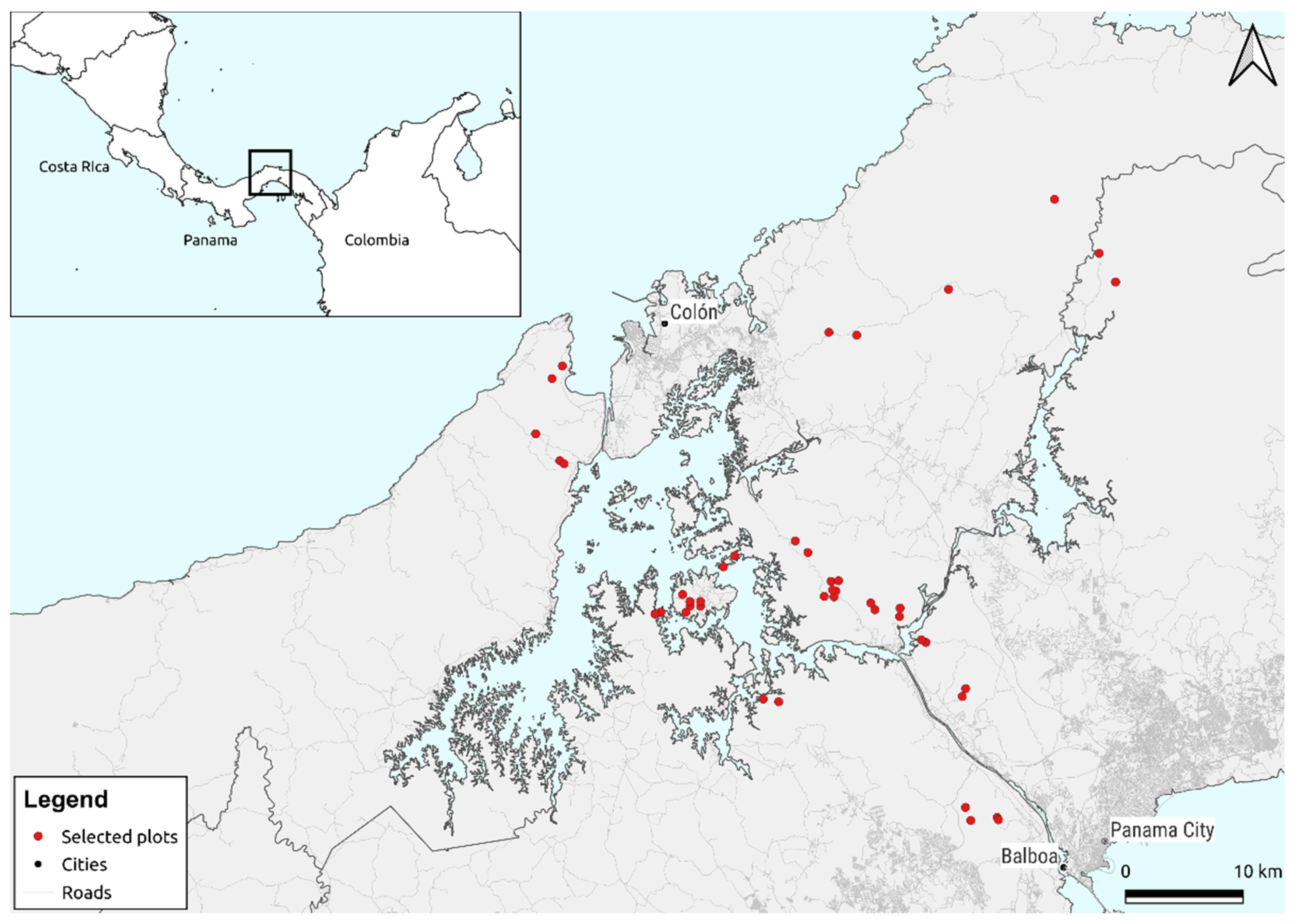
4. Comparing BetaBayes with Mantel Tests and Generalised Dissimilarity Modelling

To demonstrate the use of BetaBayes and compare its results with those from Mantel tests and generalised dissimilarity modelling, we chose a dataset collected by Condit et al. [36] available as supplementary information on the publication’s website. The dataset contains information on multiple 1 ha plots from rain forests in Panama, Ecuador, and Peru, where all plants with a stem diameter higher than 10 cm were identified at the species level. In our study, we only used data from Panama. Condit et al. [36] observed that community similarity measured by Sorensen’s similarity index decays with distance. Subsequent studies analysed parts of this dataset using Mantel tests and generalised dissimilarity modelling. Chust et al. [37] worked with 53 plots from Panama and used Mantel tests to assess the correlation between Jaccard and Steinhaus similarity indices, geographic distance, and environmental factors, such as elevation, slope, and climate variables. They observed that community similarity declined with increasing geographic distance and differences in topographical and climate variables. Ferrier et al. [9] used 43 plots from Panama to exemplify the use of GDM, having found strong positive associations between community dissimilarity, geographic distance, and differences in elevation and precipitation. For this analysis, we selected 43 plots located in Panama at least 400 m apart but no more than 60 km (Figure 1). We calculated the Bray–Curtis indices [38] between all pairs of plots and considered two covariates, geographic distance and elevation.

4.1. Mantel Test

To run Mantel tests, we used the function mantel() from the R package “vegan” [39]. The results from the tests suggested there were significant positive correlations between Bray–Curtis dissimilarity indices, geographical distance (r = 0.586, p-value = 0.001), and differences in elevation (r = 0.355, p = 0.001) (Supplementary Material—Sections S1–S4).

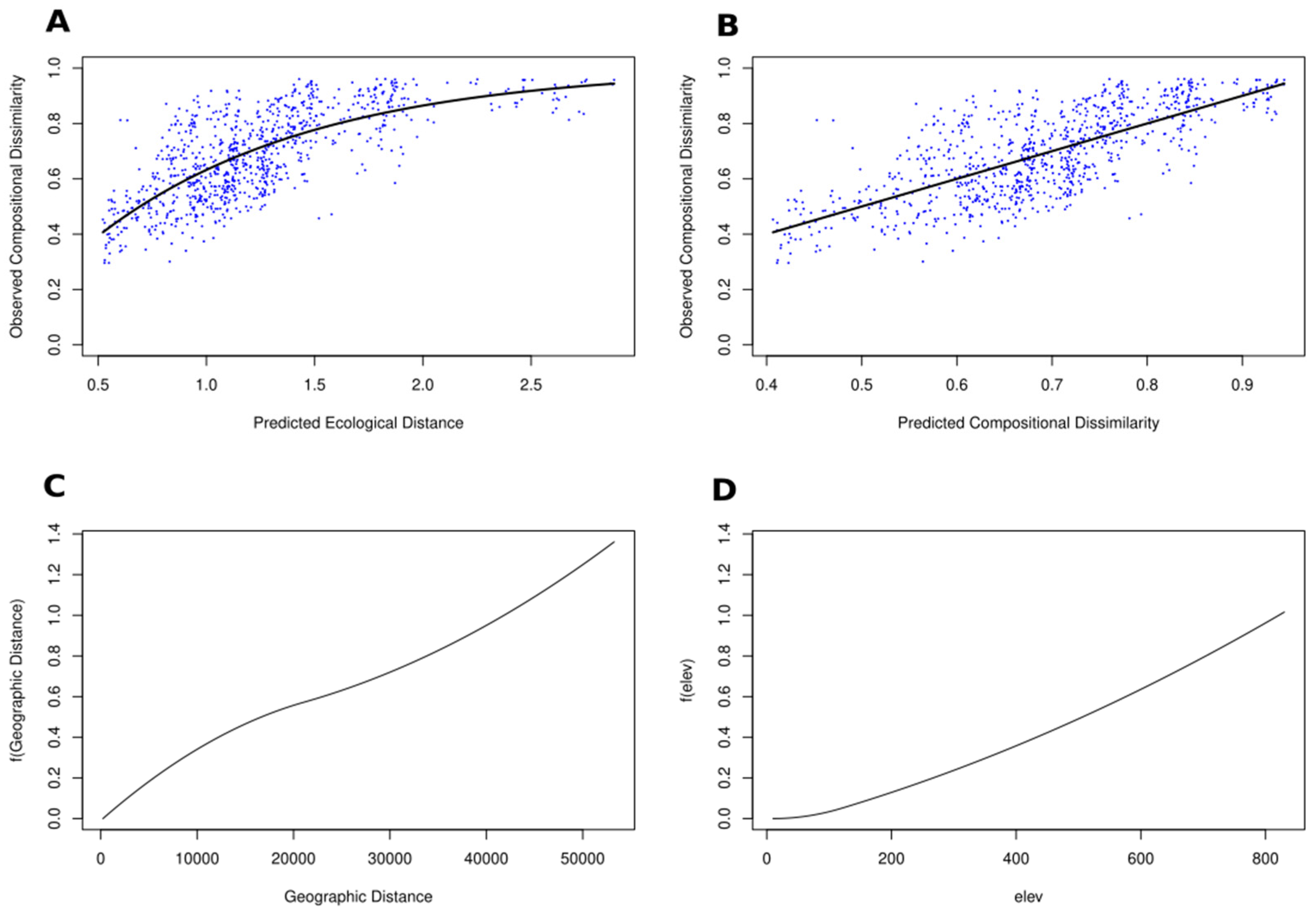
4.2. Generalised Dissimilarity Modelling

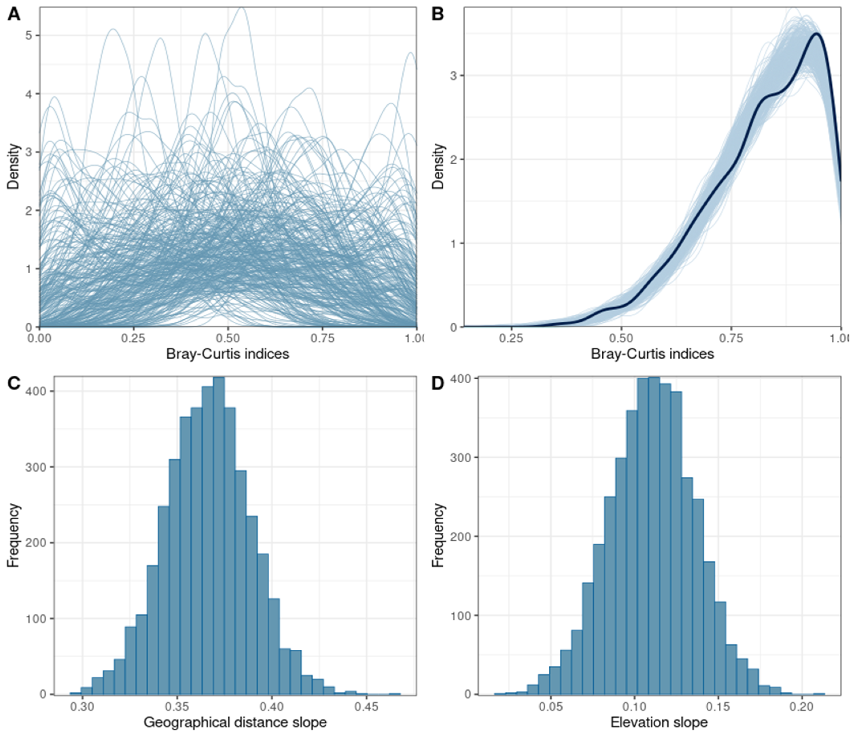
We used the R package “gdm” [40] to implement the generalised dissimilarity model. The resulting model explained 52.51% of the deviance and provided a good match between observed and predicted compositional similarity (Figure 2B), showing that the model fit the data well. The permutation tests returned p-values < 0.05 for both predictors, which suggested that the model considered them both significant even after accounting for the non-independence of Bray–Curtis indices. The spline function for geographical distance attained the highest maximum transformed value (1.37), indicating it was the most important predictor. The spline for elevation reached a slightly lower value (1.023), demonstrating it was also an important predictor. Overall, the model suggested that compositional dissimilarity grew rapidly with increasing ecological distance but then the growth decelerated (Figure 2A).

4.3. BetaBayes

Since Bray–Curtis indices are constrained between 0 and 1, we had to make minor modifications to the model we presented earlier. We replaced the normal distribution with a beta distribution, which is a continuous probability distribution defined in the interval 0 and 1. We parameterised the beta distribution by the mean (or location) μ and sample size κ [32]. To ensure the parameter μ was bound between 0 and 1, we modelled the logit of μ in a linear model of the covariates. We implemented BetaBayes using Stan’s probabilistic programming language [26] in CmdStan, the software R 4.2 [33], and the R package CmdStanR [34], which provides an R interface for CmdStan.

The model was then:

Beta diversity index_i,j ~ Beta distribution (μ_ij, κ)

logit (μ_ij) = α + α_s,i + α_s,j + β₁ * Geographical distance + β₂ * Elevation difference

α ~ Normal (0, 0.3)

α_s ~ Normal (0, σ_s)

σ_s ~ Exponential (1)

β₁, β₂ ~ Normal (0, 1)

κ ~ Half-Normal (0, 50)

We chose a weakly informative prior model that assigns a slightly higher probability to distributions of Bray–Curtis indices centred around 0.5 but that also assigns high probability to distributions concentrated around higher and lower values (Figure 3A). We transformed both covariates to improve model fit, identifiability, and runtime. We transformed geographical distance by subtracting 10 km from the observed values and dividing the resulting value by 10 km. As for the difference in elevation, we subtracted 100 m and then divided the result by 100 m.

The chains were stationary and well mixed with Rhat values of ~1 (Supplementary Material S1—Section S6.4). No iterations ended with divergences or saturated the maximum tree depth. The posterior distribution of Bray–Curtis indices closely matched the observed distribution, except for values below 0.39, which were slightly overestimated (Figure 3B and Supplementary Material S1). Our prior model regularized inferences of Bray–Curtis indices towards 0.5, which can introduce an apparent bias when there are only a small number of observations. That said, the observed bias was typically within the posterior uncertainties and so was not practically significant. Moreover, as more data are introduced, the likelihood function dominates the structure of the posterior distribution, and this prior bias weakens automatically. The posterior distributions of the slope parameters for geographical distance and elevation do not cross zero, suggesting a strong association between Bray–Curtis indices and these two covariates. The geographical distance slope had the highest mean value (0.366) and a 95% credibility interval of [0.323, 0.381], which indicated it was the strongest predictor. This meant that when geographical distances increased from the baseline value of 10 km to 20 km, the expected logit Bray–Curtis index could increase by approximately 0.366. The elevation slope had a mean estimate of 0.109 with a 95% credibility interval of [0.058, 0.160], indicating that when elevation difference increased from the baseline value of 100 m to 200 m, the expected logit Bray–Curtis index increased by 0.109.

5. BetaBayes Extensions

BetaBayes is an extremely flexible framework for modelling changes in community similarity or dissimilarity that can easily be adapted to the particular structure of data. In this section, we demonstrate how BetaBayes can incorporate varying effects (i.e., random effects), spatial autocorrelation, and highly nonlinear relationships.

5.1. Varying Effects

Varying effects allow the model to account for discrete heterogeneity that is constant over time and not correlated to the independent variables [34,41]. For example, if we believe the relationship between beta diversity indices and covariates can change across data clusters (i.e., regions), we can add varying intercepts α_c[cluster] and varying slopes β_c[cluster] that change across data clusters.

S ~ Normal (μ, σ)

μ = α + α_s,i + α_s,j + α_c[cluster] + β_[cluster]C

α ~ Normal (10, 1)

α_s ~ Normal (0, σ_s)

α_c[cluster] ~ Normal (0, 1)

β_[cluster] ~ Normal (0, 1)

α_s ~ Normal (0, σ_s);

In a recent paper [31], we used this approach to analyse how community similarity among riparian plant communities changes as a function of neutral and niche-based covariates. We worked with 338 communities located in 11 river basins. We added varying effects to the model, which allowed us to examine how the relationship between community similarity and covariates changed across different river basins.

5.2. Spatial Autocorrelation

Communities that are closer to each other are more likely to be similar in terms of species composition than those that are further apart [42,43]. To account for spatial autocorrelation between beta diversity indices, we can use a spatial model, such as a Markov random field or a Gaussian process. For example, in a Gaussian process model, we would estimate unique intercepts for every distance value while still considering distance as a continuous dimension in which similar distances correspond to more similar intercepts [20]. We can formulate the model as follows:

S ~ Normal (μ, σ)

μ = α + α_s,i + α_s,j + βC + K_[cluster]

α ~ Normal (10, 1)

α_s ~ Normal (0, σ_s)

β ~ Normal (0, 1)

K ~ Multivariate Normal (vector (n, 0), K_ij)

K_ij = η²exp(−ρ² D²_ij) + δ_ijσ²

η² ~ Exponential (2)

ρ² ~ Exponential (0.5)

Where C is the varying intercept, which is estimated considering geographic distance. The prior for this parameter is an n-dimensional multivariate normal distribution, where n is equal to the number of clusters and K_ij is the covariance between any pair of communities i and j. The formula for K_ij models how the covariance among communities changes with the distances between them. In this example, we chose a formula that assumes the covariance between communities i and j declines exponentially with the squared distance between them. The rate of decline is determined by the parameter ρ: if it is large, then the covariance declines more rapidly with the squared distance.

5.3. Complex Nonlinear Relationships

In the Panama dataset, we observed a moderately nonlinear relationship between community dissimilarity and covariates that our model could accommodate. However, if we observe complex nonlinear relationships, we have to make some changes. We can use splines, which are smooth functions built out of smaller component functions [22]. We can exemplify this by using basis splines (B-splines). B-splines build up wiggly functions from simpler, less-wiggly components called basis functions. In short, B-splines divide the full range of a predictor variable into parts, assigning a parameter to each of those parts. The parameters are gradually switched on and off, making a wiggly curve. The model is then:

S_i ~ Normal (μ, σ)

μ_i = α + α_s,i + α_s,j + w₁B_i,1 + w₂B_i,2

w_1,w₂ ~ Normal (0, 10)

α ~ Normal (0, 1)

α_s ~ Normal (0, σ_s)

σ ~ Exponential (1)

Where B_i,n is the n-th basis function’s value on row i, and the w_i parameters are the corresponding weights for each function. The B parameters work like regular slopes, adjusting the influence of each basis function on the mean μ_i.

6. Conclusions

BetaBayes is a powerful and flexible framework for modelling changes in community dissimilarity measured by beta diversity indices that specifically incorporates the dependence among indices. BetaBayes is based on the Bradley–Terry model, which was developed for modelling paired comparisons and often used in sports science [44], economics [26], and machine learning [29,45]. The Bradley–Terry model is a time-tested approach whose robustness is supported by multiple simulation studies covering a wide range of data-dependence scenarios [46,47,48].

BetaBayes has two distinctive features. The first is its flexibility. BetaBayes is not a method but a framework that can be adapted to fit the structure of data. In Section 5, we explained how it can accommodate varying effects and spatial autocorrelation and fit complex nonlinear relationships. BetaBayes leverages the power and flexibility of Stan’s probabilistic programming language, which allows the user to fit a wide range of models without having to rely on multiple software packages. The second advantage of BetaBayes is that it provides a clear path for performing model validation. Bayesian models are generative, meaning that we can generate predicted data from the posterior distribution and compare it with the observed data. This procedure makes it possible to determine if the model captures the data’s relevant structure and to improve it if necessary. In the presented example with the Panama dataset, we demonstrated how the user can check if the model is consistent with the observed data.

BetaBayes avoids hypothesis testing entirely and instead focuses on collecting information into inferences about the observed data. This approach requires first replicating the data-generating process that generated the paired comparisons and then quantifying which model configurations are consistent with the observed data. In particular, BetaBayes aims to capture the uncertainty in inferences, quantifying all the model configurations consistent with the data and not just a select few. Although this approach requires far more work than competing methods, its results are far more transparent and far easier to validate.

References

1. Chang, C.C.; Turner, B.L. Ecological Succession in a Changing World. J. Ecol. 2019, 107, 503–509. [Google Scholar] [CrossRef] [Green Version]
2. Hubbell, S. The Unified Neutral Theory of Biodiversity and Biogeography; Princeton University Press: Princeton, NJ, USA, 2001; ISBN 978-0-691-02128-7. [Google Scholar]
3. Magurran, A.E.; Deacon, A.E.; Moyes, F.; Shimadzu, H.; Dornelas, M.; Phillip, D.A.T.; Ramnarine, I.W. Divergent Biodiversity Change within Ecosystems. Proc. Natl. Acad. Sci. USA 2018, 115, 1843–1847. [Google Scholar] [CrossRef] [PubMed] [Green Version]
4. Pereira, H.M.; Navarro, L.M.; Martins, I.S. Global Biodiversity Change: The Bad, the Good, and the Unknown. Annu. Rev. Environ. Resour. 2012, 37, 25–50. [Google Scholar] [CrossRef] [Green Version]
5. Ferrier, S.; Guisan, A. Spatial Modelling of Biodiversity at the Community Level. J. Appl. Ecol. 2006, 43, 393–404. [Google Scholar] [CrossRef]
6. D’Amen, M.; Rahbek, C.; Zimmermann, N.E. Spatial Predictions at the Community Level: From Current Approaches to Future Frameworks. Biol. Rev. 2017, 92, 169–187. [Google Scholar] [CrossRef]
7. Graco-Roza, C.; Aarnio, S.; Abrego, N.; Acosta, A.T.R.; Alahuhta, J.; Altman, J.; Angiolini, C.; Aroviita, J.; Attorre, F.; Baastrup-Spohr, L.; et al. Distance Decay 2.0—A Global Synthesis of Taxonomic and Functional Turnover in Ecological Communities. Glob. Ecol. Biogeogr. 2022, 31, 1399–1421. [Google Scholar] [CrossRef]
8. MacKenzie, D.I.; Nichols, J.D.; Royle, J.A.; Pollock, K.H.; Bailey, L.; Hines, J.E. Occupancy Estimation and Modeling: Inferring Patterns and Dynamics of Species Occurrence, 2nd ed.; Academic Press: London, UK, 2017; ISBN 978-0-12-814691-0. [Google Scholar]
9. Ferrier, S.; Manion, G.; Elith, J.; Richardson, K. Using Generalized Dissimilarity Modelling to Analyse and Predict Patterns of Beta Diversity in Regional Biodiversity Assessment. Divers. Distrib. 2007, 13, 252–264. [Google Scholar] [CrossRef]
10. Pollock, L.J.; O’Connor, L.M.J.; Mokany, K.; Rosauer, D.F.; Talluto, M.V.; Thuiller, W. Protecting Biodiversity (in All Its Complexity): New Models and Methods. Trends Ecol. Evol. 2020, 35, 1119–1128. [Google Scholar] [CrossRef]
11. Viana, D.S.; Keil, P.; Jeliazkov, A. Disentangling Spatial and Environmental Effects: Flexible Methods for Community Ecology and Macroecology. Ecosphere 2022, 13, e4028. [Google Scholar] [CrossRef]
12. Mokany, K.; Ware, C.; Woolley, S.N.C.; Ferrier, S.; Fitzpatrick, M.C. A Working Guide to Harnessing Generalized Dissimilarity Modelling for Biodiversity Analysis and Conservation Assessment. Glob. Ecol. Biogeogr. 2022, 31, 802–821. [Google Scholar] [CrossRef]
13. Legendre, P.; Borcard, D.; Peres-Neto, P.R. Analyzing Beta Diversity: Partitioning the Spatial Variation of Community Composition Data. Ecol. Monogr. 2005, 75, 435–450. [Google Scholar] [CrossRef]
14. Mantel, N. The Detection of Disease Clustering and a Generalized Regression Approach. Cancer Res. 1967, 27, 209–220. [Google Scholar] [PubMed]
15. Smouse, P.E.; Long, J.C.; Sokal, R.R. Multiple Regression and Correlation Extensions of the Mantel Test of Matrix Correspondence. Syst. Zool. 1986, 35, 627–632. [Google Scholar] [CrossRef]
16. Legendre, P. Comparison of Permutation Methods for the Partial Correlation and Partial Mantel Tests. J. Stat. Comput. Simul. 2000, 67, 37–73. [Google Scholar] [CrossRef]
17. Guillot, G.; Rousset, F. Dismantling the Mantel Tests. Methods Ecol. Evol. 2013, 4, 336–344. [Google Scholar] [CrossRef] [Green Version]
18. Legendre, P.; Fortin, M.-J.; Borcard, D. Should the Mantel Test Be Used in Spatial Analysis? Methods Ecol. Evol. 2015, 6, 1239–1247. [Google Scholar] [CrossRef]
19. Crabot, J.; Clappe, S.; Dray, S.; Datry, T. Testing the Mantel Statistic with a Spatially-Constrained Permutation Procedure. Methods Ecol. Evol. 2019, 10, 532–540. [Google Scholar] [CrossRef]
20. McElreath, R. Statistical Rethinking: A Bayesian Course with Examples in R and Stan, 2nd ed.; Chapman and Hall/CRC: Boca Raton, FL, USA, 2020. [Google Scholar]
21. Ferrier, S.; Drielsma, M.; Manion, G.; Watson, G. Extended Statistical Approaches to Modelling Spatial Pattern in Biodiversity in Northeast New South Wales. II. Community-Level Modelling. Biodivers. Conserv. 2002, 11, 2309–2338. [Google Scholar] [CrossRef]
22. Woolley, S.N.C.; Foster, S.D.; O’Hara, T.D.; Wintle, B.A.; Dunstan, P.K. Characterising Uncertainty in Generalised Dissimilarity Models. Methods Ecol. Evol. 2017, 8, 985–995. [Google Scholar] [CrossRef] [Green Version]
23. Koleff, P.; Gaston, K.J.; Lennon, J.J. Measuring Beta Diversity for Presence–Absence Data. J. Anim. Ecol. 2003, 72, 367–382. [Google Scholar] [CrossRef]
24. Bradley, R.A.; Terry, M.E. Rank Analysis of Incomplete Block Designs: I. The Method of Paired Comparisons. Biometrika 1952, 39, 324–345. [Google Scholar] [CrossRef]
25. Zermelo, E. Die Berechnung der Turnier-Ergebnisse als ein Maximumproblem der Wahrscheinlichkeitsrechnung. Math. Z. 1929, 29, 436–460. [Google Scholar] [CrossRef]
26. Agresti, A. Categorical Data Analysis, 3rd ed.; Wiley: Hoboken, NJ, USA, 2012; ISBN 978-0-470-46363-5. [Google Scholar]
27. McHale, I.; Morton, A. A Bradley-Terry Type Model for Forecasting Tennis Match Results. Int. J. Forecast. 2011, 27, 619–630. [Google Scholar] [CrossRef]
28. Koehler, K.J.; Ridpath, H. An Application of a Biased Version of the Bradley-Terry-Luce Model to Professional Basketball Results. J. Math. Psychol. 1982, 25, 187–205. [Google Scholar] [CrossRef]
29. Hunter, D.R. MM Algorithms for Generalized Bradley-Terry Models. Ann. Stat. 2004, 32. [Google Scholar] [CrossRef]
30. Jeon, J.-J.; Kim, Y. Revisiting the Bradley-Terry Model and Its Application to Information Retrieval. J. Korean Data Inf. Sci. Soc. 2013, 24, 1089–1099. [Google Scholar] [CrossRef] [Green Version]
31. Rodríguez Montequín, V.; Villanueva Balsera, J.M.; Díaz Piloñeta, M.; Álvarez Pérez, C. A Bradley-Terry Model-Based Approach to Prioritize the Balance Scorecard Driving Factors: The Case Study of a Financial Software Factory. Mathematics 2020, 8, 276. [Google Scholar] [CrossRef] [Green Version]
32. Ehrlich, J.; Potter, J.; Sanders, S. The Effect of Attendance on Home Field Advantage in the National Football League: A Natural Experiment; Syracuse University: Syracuse, NY, USA, 2021. [Google Scholar]
33. Gabry, J.; Simpson, D.; Vehtari, A.; Betancourt, M.; Gelman, A. Visualization in Bayesian Workflow. J. R. Stat. Soc. Ser. A Stat. Soc. 2019, 182, 389–402. [Google Scholar] [CrossRef] [Green Version]
34. Gelman, A.; Carlin, J.B.; Stern, H.S.; Dunson, D.B.; Vehtari, A.; Rubin, D.B. Bayesian Data Analysis, 3rd ed.; Chapman and Hall/CRC: Boca Raton, FL, USA, 2013; ISBN 978-1-4398-4095-5. [Google Scholar]
35. Stan Development Team. Stan Modeling Language Users Guide and Reference Manual, Version 2.2.4; 2020. Available online: http://mc-stan.org (accessed on 10 December 2021).
36. Condit, R.; Pitman, N.; Leigh, E.G.; Chave, J.; Terborgh, J.; Foster, R.B.; Núñez, P.; Aguilar, S.; Valencia, R.; Villa, G.; et al. Beta-Diversity in Tropical Forest Trees. Science 2002, 295, 666–669. [Google Scholar] [CrossRef] [Green Version]
37. Chust, G.; Chave, J.; Condit, R.; Aguilar, S.; Lao, S.; Pérez, R. Determinants and Spatial Modeling of Tree Β-diversity in a Tropical Forest Landscape in Panama. J. Veg. Sci. 2006, 17, 83–92. [Google Scholar] [CrossRef]
38. Bray, J.R.; Curtis, J.T. An Ordination of the Upland Forest Communities of Southern Wisconsin. Ecol. Monogr. 1957, 27, 325–349. [Google Scholar] [CrossRef]
39. Oksanen, J.; Blanchet, F.G.; Friendly, M.; Kindt, R.; Legendre, P.; McGlinn, D.; Minchin, P.R.; O’Hara, R.B.; Simpson, G.L.; Solymos, P.; et al. Vegan: Community Ecology Package—Version 2.7-7. 2021. Available online: http://CRAN.R-project.org/package=vegan (accessed on 12 December 2021).
40. Fitzpatrick, M.; Mokany, K.; Manion, G.; Nieto-Lugilde, D.; Ferrier, S. gdm: Generalized Dissimilarity Modeling 2022. Available online: https://cran.r-project.org/web/packages/gdm/index.html (accessed on 12 May 2022).
41. Pinheiro, J.; Bates, D. Mixed-Effects Models in S and S-PLUS; Springer: New York, NY, USA, 2009; ISBN 1-4419-0317-8. [Google Scholar]
42. Morlon, H.; Chuyong, G.; Condit, R.; Hubbell, S.; Kenfack, D.; Thomas, D.; Valencia, R.; Green, J.L. A General Framework for the Distance-Decay of Similarity in Ecological Communities. Ecol. Lett. 2008, 11, 904–917. [Google Scholar] [CrossRef] [Green Version]
43. Soininen, J.; McDonald, R.; Hillebrand, H. The Distance Decay of Similarity in Ecological Communities. Ecography 2007, 30, 3–12. [Google Scholar] [CrossRef]
44. Cattelan, M.; Varin, C.; Firth, D. Dynamic Bradley–Terry Modelling of Sports Tournaments. J. R. Stat. Soc. Ser. C Appl. Stat. 2013, 62, 135–150. [Google Scholar] [CrossRef] [Green Version]
45. Menke, J.E.; Martinez, T.R. A Bradley–Terry Artificial Neural Network Model for Individual Ratings in Group Competitions. Neural Comput. Appl. 2008, 17, 175–186. [Google Scholar] [CrossRef]
46. Yan, T. Ranking in the Generalized Bradley–Terry Models When the Strong Connection Condition Fails. Commun. Stat. Theory Methods 2016, 45, 340–353. [Google Scholar] [CrossRef] [Green Version]
47. Shev, A.; Fujii, K.; Hsieh, F.; McCowan, B. Systemic Testing on Bradley-Terry Model against Nonlinear Ranking Hierarchy. PLoS ONE 2014, 9, e115367. [Google Scholar] [CrossRef] [Green Version]
48. Stern, S.E. Moderated Paired Comparisons: A Generalized Bradley-Terry Model for Continuous Data Using a Discontinuous Penalized Likelihood Function. J. R. Stat. Soc. Ser. C Appl. Stat. 2011, 60, 397–415. [Google Scholar] [CrossRef]
Figure 1. The red dots represent the locations of the 43 vegetation plots from Condit et al. [36] that were selected for this study.
Diversity 14 00858 g001
Figure 2. (A) Observed dissimilarity as a function of GDM-predicted ecological distance, with each pair of sites represented by a point. The dark line represents the GDM-predicted dissimilarity. (B) Observed dissimilarity as a function of GDM-predicted dissimilarity, and a line with slope 1. (C) Spline function for geographic distance and (D) spline function for elevation.
Diversity 14 00858 g002
Figure 3. (A) Density plot showing 1000 prior predictive distributions. (B) Density plot showing the observed distribution of Bray–Curtis indices (thick line) against 1000 posterior distributions (thin lines). (C) Posterior distribution of the slope parameter corresponding to the geographical distance and (D) posterior distribution of the slope parameter corresponding to the precipitation difference.
Diversity 14 00858 g003
Publisher’s Note: MDPI stays neutral with regard to jurisdictional claims in published maps and institutional affiliations.