Article

Presence and Biomass Information Extraction from Highly Uncertain Data of an Experimental Low-Range Insect Radar Setup

Faculty of Geography, Philipps University of Marburg, Deutschhausstraße 12, 35032 Marburg, Germany
*
Author to whom correspondence should be addressed.
Diversity 2021, 13(9), 452; https://doi.org/10.3390/d13090452
Submission received: 6 August 2021 / Revised: 16 September 2021 / Accepted: 17 September 2021 / Published: 21 September 2021

Abstract

:
Systematic, practicable, and global solutions are required for insect monitoring to address species decline and pest management concerns. Compact frequency-modulated continuous-wave (FMCW) radar can facilitate these processes. In this work, we evaluate a 60 GHz low-range FMCW radar device for its applicability to insect monitoring. Initial tests showed that radar parameters should be carefully selected. We defined optimal radar configuration during the first experiment and developed a methodology for individual target observation. In the second experiment, we tried various individual-insect targets, including small ones. The third experiment was devoted to mass-insect-target detection. All experiments were intentionally conducted in very uncertain conditions to make them closer to a real field situation. A novel parameter, the Sum of Sequential Absolute Magnitude Differences (SSAMD), has been proposed for uncertainty reduction and noisy data processing. SSAMD enables insect target presence detection and biomass estimation. We have defined ranges of SSAMD for distinguishing noise, insects, and other larger targets (e.g., bats, birds, or other larger objects). We have provided evidence of the high correlation between insect numbers and the average of SSAMD values proving the biomass estimation possibility. This work confirms that such radar devices can be used for insect monitoring. We plan to use the evaluated system assembled with a light trap for real fieldwork in the future.

1. Introduction

Four hundred recently extinct insect species [1], a 75% decline in total flying insect biomass in protected areas [2], the possibility of the extinction of 40% of insects over the next few decades [1], and other serious concerns have attracted strong worldwide attention to insect conservation and pest control [3] problems. Despite significant efforts, major unsolved challenges [4] indicate the high demand for systematic, grounded, and global insect monitoring solutions.
Random walks, pattern formation, synchronization, and networks are well-established approaches to insect monitoring [5]. Many works confirm the effectiveness of trapping methods that belong to classical methods [6,7,8,9]. Among them, nowadays, automatic light camera traps are starting to play a central role due to technical progress [10,11,12,13]. A modern tendency to use the camera with light traps bridges trapping approaches with remote sensing methods of insect monitoring, where sky-oriented and unmanned aerial vehicle-borne cameras are becoming more distinguishable due to the recent progress in robotics and computer vision [14,15,16]. Despite this, among remote sensing methods for insect monitoring, radar technology historically plays a central role.
Insect radar’s history started at the end of the 1940s [17]. Scanning pulsed radar was a dominating technology in the earliest works [18,19]. The signal of such systems can cover large areas; it makes them useful for monitoring large insect swarms (e.g., locusts) [20,21]. Later, vertical-looking pulsed radar sets became another primary solution [22,23,24]. Such radar sets allowed the collection of higher granulation information (in comparison to scanning systems): insects’ speed, motion direction, orientation, and several radar scattering cross-section terms related to the insect body mass and shape. The third large insect radar group is harmonic systems [25,26,27,28] using a transponder attached to an insect, allowing tracking of the target. The vast majority of state-of-the-art insect radar sets are based on pulsed systems, extensively reviewed in several works [29,30,31].
Frequency-modulated continuous-wave (FMCW) radar technology is an alternative to pulsed systems. Our recent review of achievements in insect radar [32] has distinguished the rise of FMCW insect radar solutions’ interest. It is caused by three primary factors: compactness of devices, low energy consumption, and advances in data processing. Furthermore, we have found no works on insect radar concerning systematic mass insect monitoring in the range of a few meters and tens of meters from radar. Small ranges are only considered by harmonic radar tracking tagged insects, while mass monitoring is beyond the scope of the insect radar. This niche is currently occupied by systems using cameras (modern computer vision algorithms for data processing) and lidar solutions [33]. Statutory insect radar systems aim at a much larger range (the minimum range is often around tens of meters depending on the pulse width). Indeed, it is pointless to use large and expensive pulsed systems (compared to FMCW compact sets) for low-range observations.
Despite these concerns, small-range radar for mass insect monitoring can have some apparent advantages. In comparison to video streaming or taking camera pictures with a small interval, FMCW radar can work continuously with relatively small energy consumption. Modern compact FMCW radar sets can measure and transmit data with a speed of approximately 100 Hz (i.e., 100 measurement acts per second), providing very compact datasets.
Furthermore, radar can reach the target through obstacles. For instance, Rankin et al. [34] discussed an attractive millimeter-wave radar set for insect detection in walls, floors, and ceilings using the range of around 0.5 m. Their multiple-input multiple-output (MIMO) device aims mainly at termite detection for an area of 75 × 75 mm2, providing discrimination from stationary clutter by Doppler and amplitude fluctuations due to insect movement. This radar application is very specific because it aims at hidden insects inside solid materials and is limited by a tiny volume. Nearly all other insect radar applications, including ours, concern insects in free air above the ground. Reference [34] also discussed a scanning FMCW radar set for UAV navigation in fog conditions.
Limited visibility due to unclear air (e.g., fog, smoke, or dust), darkness, and sun exposition is a major issue for camera observations; radar technology was designed to overpass these problems. Moreover, compared to a camera, radar can see multiple insect targets (including small ones) at different distances at the same time, without focusing on a concrete target. Typical limitations of cameras are that they need to focus and use a flashlight (dark time). Since radar works day and night simultaneously, it allows silent low-intrusion and low-energy-consumption 24/7 insect monitoring. Furthermore, FMCW radar can facilitate motion detection. A radar set working continuously can replace a motion detection system. Instead of having a continuously working camera, a radar system with the mentioned benefits can turn on the camera when necessary. Finally, radar generates principally another data type. This allows very long-term time series and the ability to create data at another abstraction level (e.g., instead of discrete objects, the insect quantity or biomass).
Finally, radar can provide very compact datasets. For instance, for FMCW radar, this can be simply a list of time-ordered magnitude float numbers or their derivatives. Thus, desired targets can be easily detected by applying a threshold value. This requires much fewer resources; algorithms can be short, fast, and straightforward (compared with computer vision and deep learning). This can be extremely useful for autonomous monitoring devices powered by solar panels or batteries.
We expect that FMCW compact radar sets can become popular for mass insect monitoring for pest control and conservation purposes. There are at least two unoccupied niches. First, in ranges of one–two meters, approaches with light traps can effectively utilize radar. Such solutions can use radar for data gathering or supplement the camera (e.g., for obtaining extra information or camera work control, as mentioned earlier). Second, in ranges of tens of meters, FMCW radar can fill the gap of statutory insect radar systems; due to the pulse width, X- and Ku-band radar sets have a sensitive minimum range (we have discussed this in [32]). In the present paper, we focus on the first niche (i.e., one–two meters).
In the following sections, we prove that a chosen compact FMCW radar device can facilitate small-range insect monitoring. This radar set is one of the best solutions currently available on the market for such a purpose. It was not designed for small targets (such as insects), aiming at much larger targets (i.e., humans, animals, vehicles) in low ranges (up to 15 m). Despite this, we have noticed that it can perceive even small insects. In the review [32], we have discussed that it makes sense to use low-range radar with a light trap to attract more insects. This was a reason for testing the radar with a light diffuser in this work. Using the device’s compactness, we consider exploiting it as a part of a rover (unmanned ground vehicle (UGV)) equipped with a light trap (see a mockup installation presented in Reference [32]). By this, we expand the idea of using FMCW systems with UAVs and show that it is possible.

2. Materials and Methods
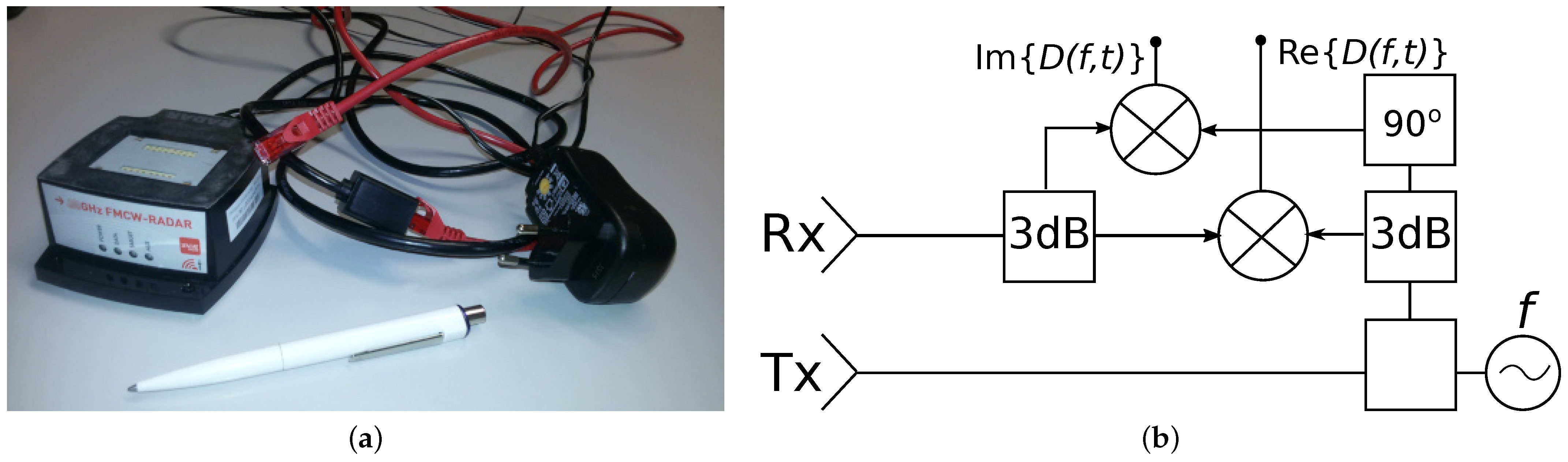
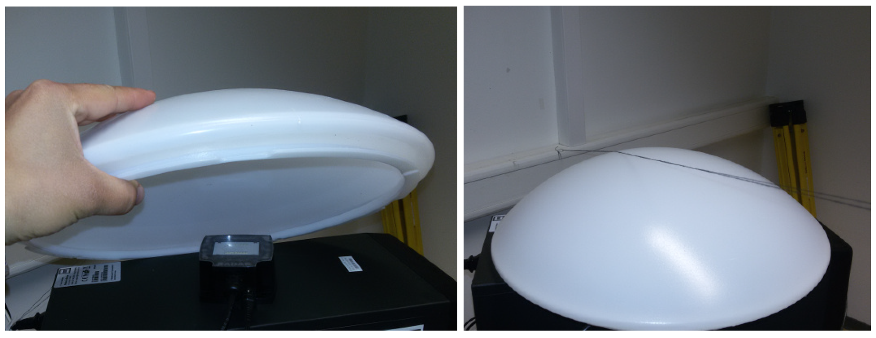
As discussed earlier, we aim to find a way to detect insects with radar at low ranges (a few meters from radar). Prior knowledge gives us optimism that this is possible. To find a solution, we have carried out several consequent experiments, described in this section. A promising approach has been found thanks to an iterative workflow.

2.1. Radar Device

In this work, we use the IMST sentire FMCW 60 GHz Radar Module; Figure 1 shows it. It is one of the most widely available radar sets that potentially allows insect detection, despite not being designed for such an aim. This subsection provides essential information from the radar’s user manual [35] since it is delivered with the device only.
According to the manual, the radar operates in FMCW or CW mode at a frequency of 60 GHz and provides the capability for range and velocity measurements in a wide area of applications. It is also possible to estimate the backscattered signal’s angle-of-arrival, corresponding to a particular target direction. The radar module is available with three different interfaces (SPI, CAN, or Ethernet). Our device provides the Ethernet interface only. The radar provides an extensive set of user commands for the following tasks:
  • configuration of radar parameters (such as the operation mode or the frequency range);
  • accessing internal radar parameters, such as the current frontend temperature or the transmission power;
  • triggering a measurement process and accessing the generated data;
  • starting high-level applications (e.g., the human tracker algorithm).
The device comprises the three following elements: (1) an interface board for the power supply and communication module, (2) baseband board for the digital signal controller and a data acquisition unit, and (3) frontend board for the radar frequency components and integrated patch antennas.
The device has one transmit (Tx) and two receive (Rx) channels. An I/Q demodulator is provided for each channel. IQ demodulation is a smart approach for reducing the amount of data without losing essential information by applying a complex baseband modulation technique with bandwidth reduction [36]. There are two independent receiver antennas for measuring the angle-of-arrival of a received signal; this feature allows the generation of a 2D reflectivity map of the illuminated scene. The radar’s antenna is linearly polarized with 65° azimuth and 24° elevation. The measurement range is 0.6–307 m; the maximal range resolution is 0.6 m. Measurement speed is ±3200 m/s, speed resolution for 1 and 100 ms modes is from 6.25 m/s to 6.25 cm/s, correspondingly. Angle measurement accuracy is 2–3°. The radar’s operation parameters are as follows: frequency ramp duration—from 1 to 100 ms, update rate—from 10 to 200 Hz, output power—from 10 to 19 dBm (tuneable), and operating temperatures are from −40 to +60 °C. The dimension (L × W × H) of the device is 97 × 87 × 42.5 mm3, and the weight is 280 g. Finally, regarding the power supply, it operates at 10.5–13 V for a regular charger and 44–54 V for Power-over-Ethernet supply [37].

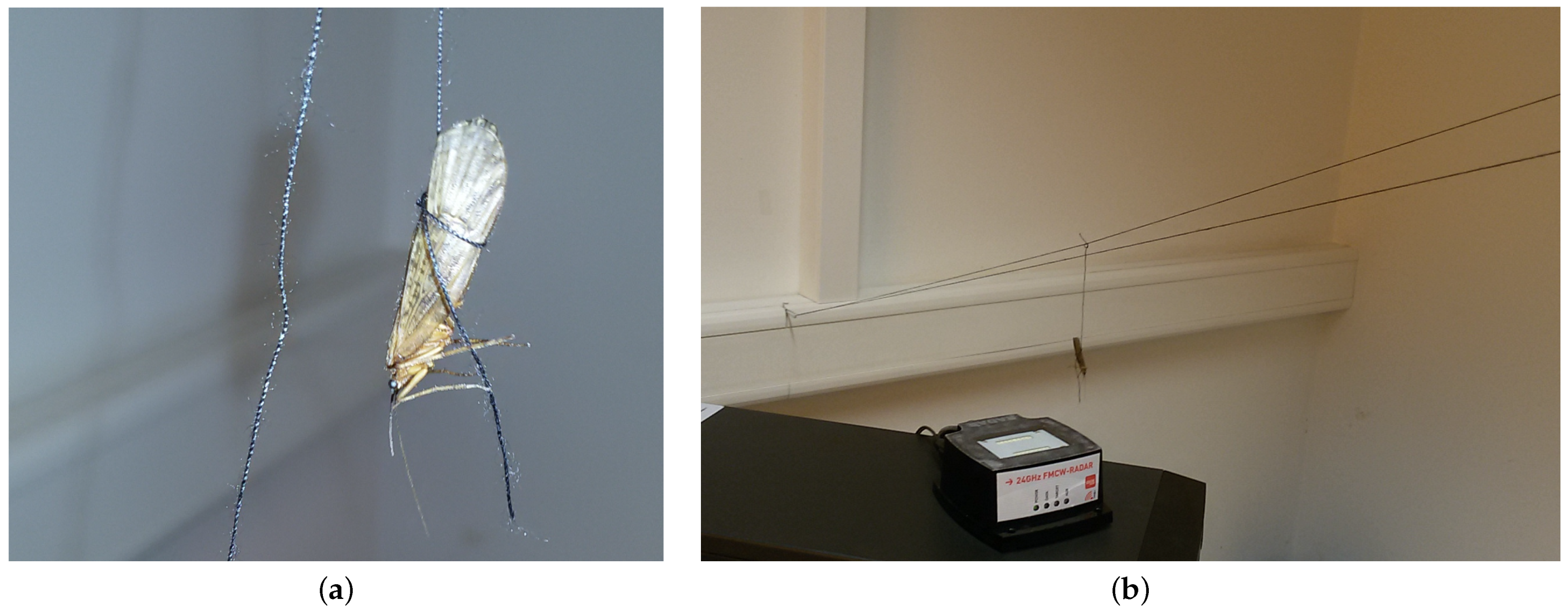
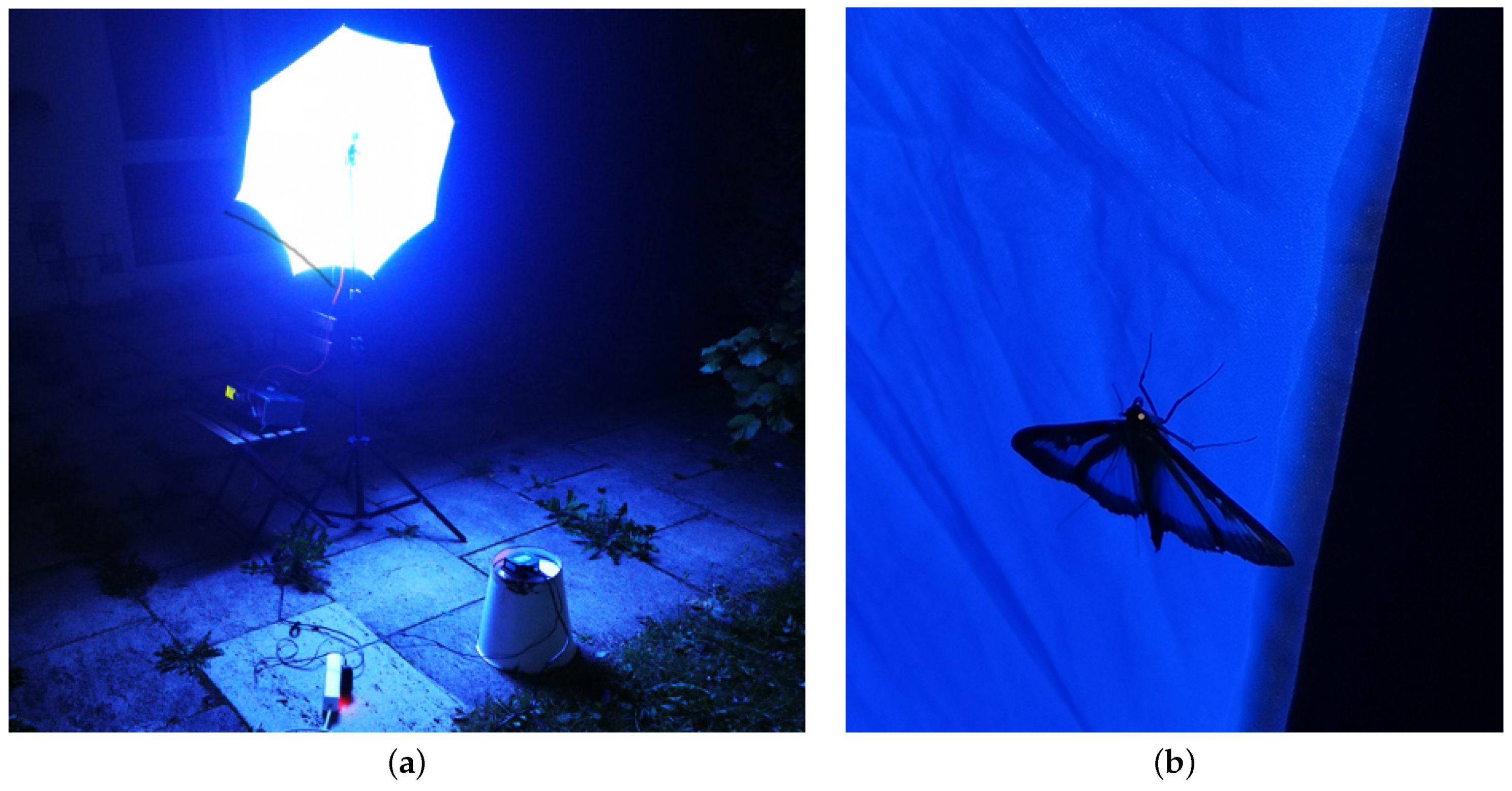
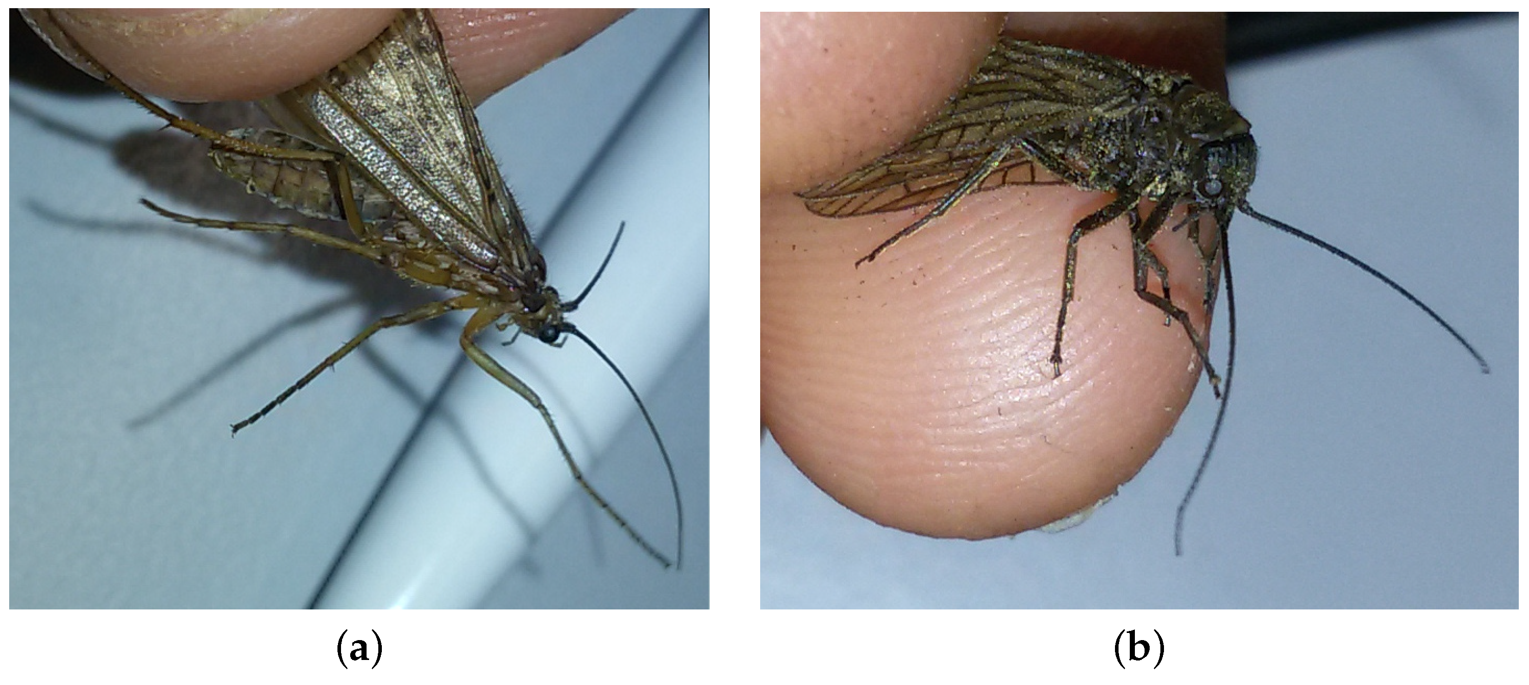
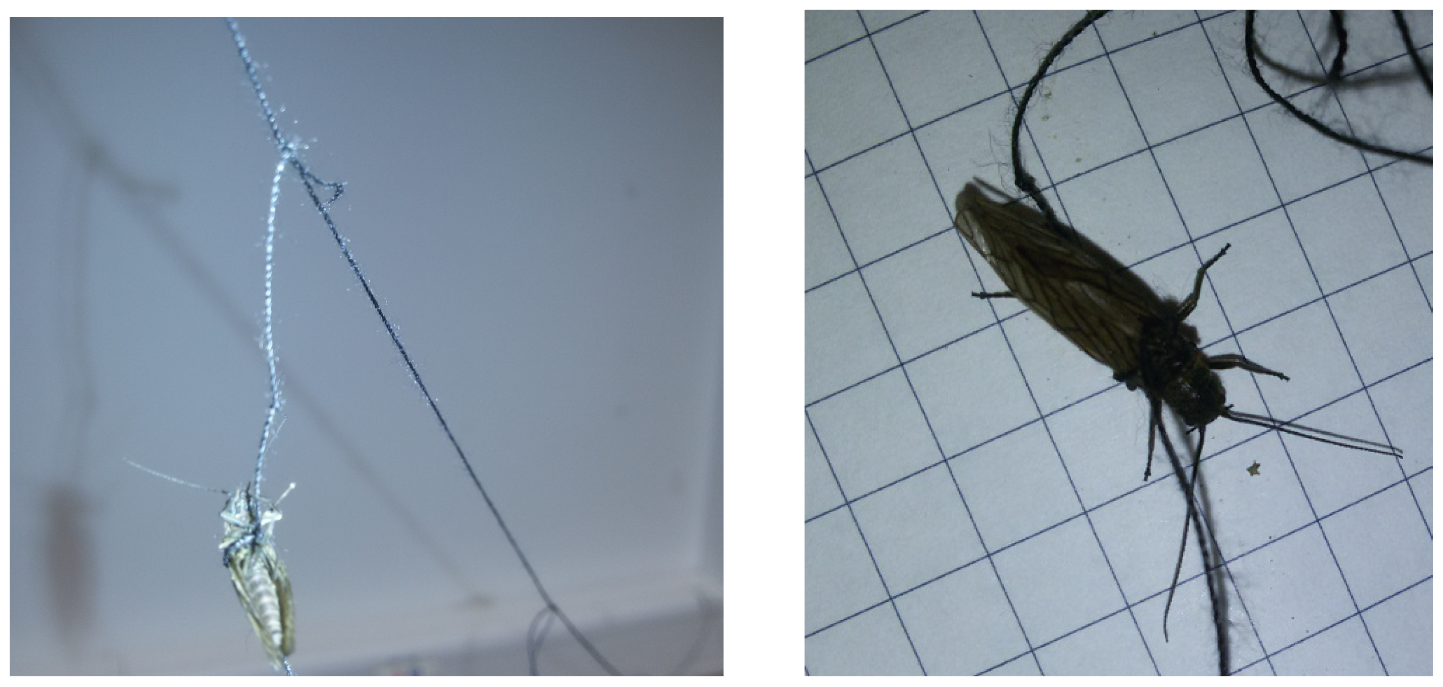
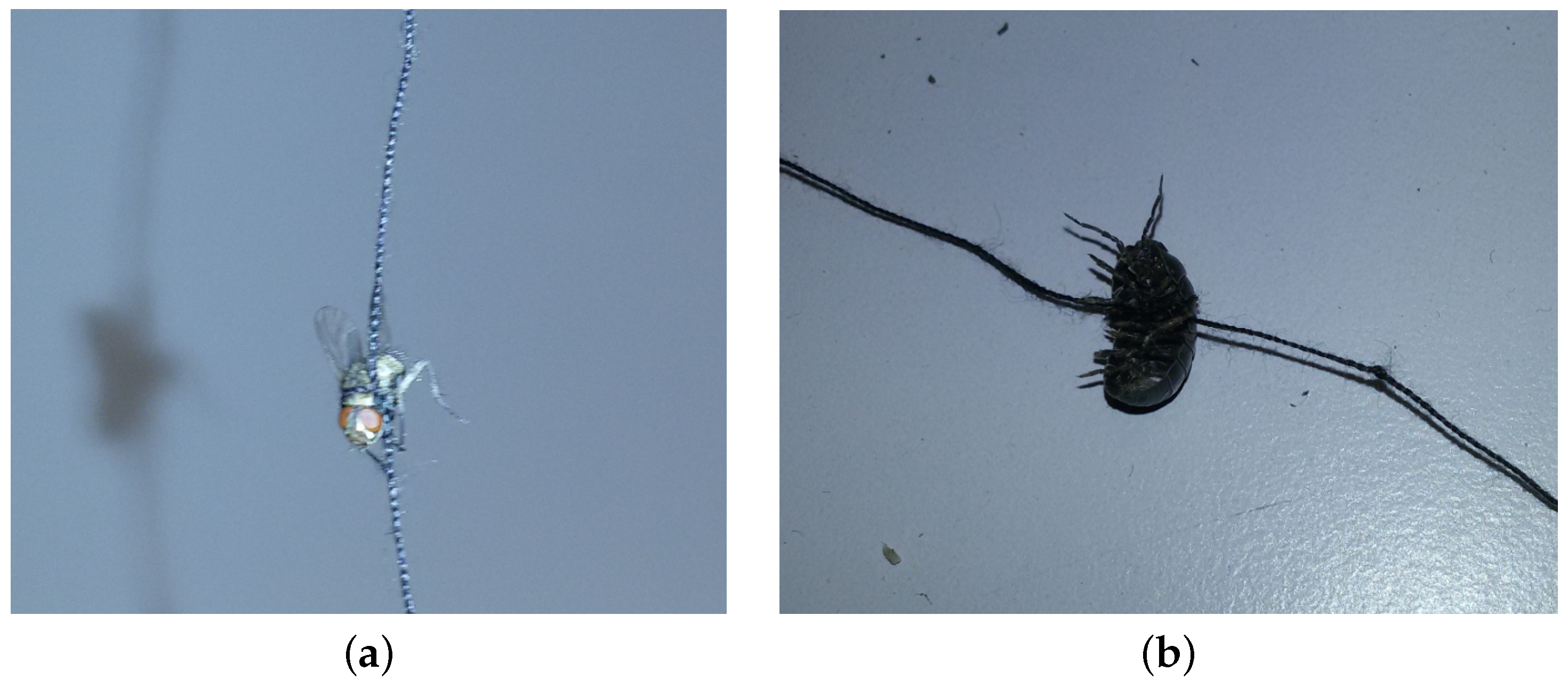
2.2. Conditions of Experiments

We have carried out a number of experiments with the discussed radar and various insects. The proposed lab setup allowed the observation of single and mass targets. We carried out an initial experiment in field conditions using a light trap to attract insects. The attempt was not successful due to non-optimal radar configuration and equipment setup. We have conducted further experiments in lab conditions.
An obvious challenge that we faced was placing the target and ensuring that the insect holder did not reflect significantly. We aimed to use live insects. Moreover, a holding technique should not damage them. For this, we tried various approaches. Most of them were not applicable because of the inability to keep the insect alive after the experiment or overly high unnecessary reflection from a holder. Finally, we found a working solution.
We noticed that normal general-purpose sewing threads made from cotton (diameter of ca. 0.3 mm) are almost invisible to the radar in any configuration during multiple tests. Even multiple connections and knots do not affect data significantly. Moreover, we noticed that a regular half-knot allows for fixing insects gently. An insect can be easily released without significant harm. Notice that all experiments were conducted in a room with 40–50% indoor humidity. We ensured that the threads were always completely dry since even slightly wet threads can reflect the radar signal significantly.
To prevent the reflection from the person conducting the experiments, we used a long thread. The middle part of the thread was held with a wall hook. An experimenter’s arms held the beginning and end parts of the thread. This allowed for pulling the thread back and forth easily. An insect was tied using a short thread connected to a long (pulled by a person) thread. Figure 2 shows the described methodology.
The insect was placed and moved at different height intervals above the radar to investigate the radar’s ability to detect such insects: H1—0–30 cm, H2—30–60 cm, H3—60–90 cm, and H4—90–120 cm. The insect moved continuously within a height interval, passing and leaving the radar-radiated zone several times. Radar measurements were monitored and recorded as multiple text files.
We have conducted two experiments using this approach. Experiment I (Figure 2) considered a Phryganea grandis insect at various height levels. Experiment II involved other species (Sialis lutaria and Acheta domesticus), including very small ones (Musca domestica and Armadillidium vulgare). Additionally, in some trials, we used a standard acrylic light diffuser, because, in the future, we want to use it as an attractive screen for a light trap. We used only single targets in both experiments for presence detection purposes. Appendix A provides a detailed description of these experiments.
Experiment III was for mass insect targets, aiming at biomass estimation of Armadillidium vulgare insects. In the previous experiment, we confirmed the presence detection ability of the radar device. During the experiments, we noticed the higher reflection from the larger insects. This means that such radar can also be used for biomass estimation.
During the third experiment, we tried to collect data confirming the biomass estimation possibility. For this, we used variable cricket numbers for two different conditions. The first condition was when crickets were placed inside the flipped diffuser. The second condition was when crickets were inside the transparent plastic packing box. All crickets had a size of around 1.5–2 cm.
Experiment IIIa. It was imperative to check how the radar worked through the diffuser. Thus, in the first attempt, we placed various numbers of insects in the flipped diffuser (see Figure 3, left). Crickets left the lowest central area of the bowl quite quickly after the placement. They crawled quickly to the edges, becoming almost unreachable by the radiating signal.
To resolve the mentioned problem and make the conditions more uncertain, we shook the diffuser with specific intervals (an interval between shaking acts). Strong and fast shaking forced the insect to fall down the central part of the diffuser. The shaking process increased the reflections dramatically. We noticed an obvious fact that with the empty bowl, the reflection signal was reduced very quickly after shaking, while, with insects, it was reduced slowly since the insects gradually left the radiating zone.
We intentionally did not attempt to create a situation where insects could not leave the radiating zone because this would make the conditions more similar to those of the future field observations when insects can freely enter and leave the radiating zone.
The following steps were conducted: (1) starting with the empty bowl (0 objects), (2) adding two insects (2 objects in the bowl), (3) adding two insects (4 objects), (4) adding four insects (8 objects), (5) adding four insects (12 objects), (6) adding four insects (16 objects), (7) adding four insects (20 objects), (8) removing five insects (15 objects), (9) removing five insects (10 objects), (10) removing five insects (5 objects), (11) removing four insects (1 object), and (12) removing the last insects (repeating the procedure with the empty bowl).
To increase the uncertainty, we implemented each step with different conditions. This means that we used a variable number of shaking acts (from 0 to tens) and non-exact intervals (typically, from 5 to 10 s) between shaking acts. Sometimes, we completed recording shortly after shaking, but for other steps, a much longer time period was left (keeping the bowl at rest). In the next section, charts show concrete conditions of each step.
Experiment IIIb. We used a transparent plastic packing box for the second part of the experiment (see Figure 3, right). In this part, insects remained relatively calm compared to the previous part (i.e., Experiment IIIa). Shaking was not required here. In such conditions, insects could leave the radiating zone, but some of them remained radiated most of the time. This led to relatively natural conditions when insects behaved relatively randomly.
In comparison to Experiment IIIa, insects did not crawl continuously to the upper edges (because of the flat bottom of the box, they felt calmer); the experiment conditions were much more straightforward. The radar device was turned on after installing the box. This means that, in contrast to the previous part, there were no external intrusions (e.g., shaking acts). The radar device worked for approximately 30 s for every step. The following steps were conducted: (1) zero, (2) one, (3) five, (4) ten, (5) fifteen, (6) twenty, (7) five, and (8) zero insects.

2.3. Sum of Sequential Absolute Magnitude Differences for Uncertainty Reduction

As discussed earlier, our radar device does not aim at such small targets as insects. During the experiments, we observed targets as noise dynamics of amplitude measurements (where increasing dynamics means appearing targets). Moreover, the intensity correlated directly with the biomass.
During the experiments, we noticed that frequency-domain data provide the most specific and valuable information. Therefore, we use only this datatype in the present work.
The radar collects data as a list of received reflections (magnitudes) ordered by the distance from the radar. It is possible to set up a maximal distance; we used 1 m. For every time moment, the radar’s software creates a separate text file. A file contains metadata, including all set parameters and an exact time. We use all four available channels. The radar was set to generate 20 files per second.
To represent these data in a usable form, we have designed a novel parameter, which has been called the Sum of Sequential Absolute Magnitude Differences ( S S A M D ). It uses the following principle:
S S A M D = t = 1 t m a x c = 1 c m a x d = 0 d m a x | m t , c , d m t 1 , c , d |
where t is a time moment or a file number ordered by time; t m a x depends on a time interval defined by the user (we use 1 s interval, so t m a x = 1 s/50 ms = 20. c is a channel number (in our case, c { 1 , 2 , 3 , 4 } , i.e., all available channels and c m a x = 4 ). d is a distance (an index of a magnitude in a list of magnitudes ordered by the distance); in our case, d m a x = 42 . m is a magnitude value. One can mention that an absolute difference between the current and previous moment is calculated. S S A M D is simply a sum of all absolute differences. In other words, the parameter calculates aggregated magnitude differences in a considered time interval, representing the observed noise dynamics as a single integer value.
Notice that S S A M D is calculated for a predefined time interval. Its meaning can be expressed as an aggregated difference of time-ordered magnitudes (dBm) in a time interval. Notice that the difference is calculated only for elements between a considered time moment and a previous time moment. Nothing can be calculated for data consisting of only one time moment (a single file).
For Experiment III data interpretation, we propose to use S S A M D ¯ (mean S S A M D or S S A M D divided by the measuring duration in seconds). This parameter can be used for biomass estimation through comparison of data taken in different conditions—in our case, various numbers of insects, different duration of an experimental step, different times of shaking acts, and time intervals between them.
In the next section, we present results obtained with the S S A M D and S S A M D ¯ parameters.

3. Results

Each experiment contains several trials. “Trial” refers to the continuous recording of the same target at the same height interval. Trials are denoted with an trial ID (from 1 to 35) and a short description in parentheses. The three following types of descriptions are applicable: (a) a height interval (“H1”, “H2”, “H3”, or “H4”), (b) the number of insects, (c) or, in some cases, letters “A” or “B” to distinguish similar trials. Examples of IDs: “3(H3)” means the third trial (an insect is in the H3 height interval); “32(20)” is for 20 insects during the 32nd act. Height intervals are only used in the first and second experiments, while insect numbers are applicable for only the third experiment.

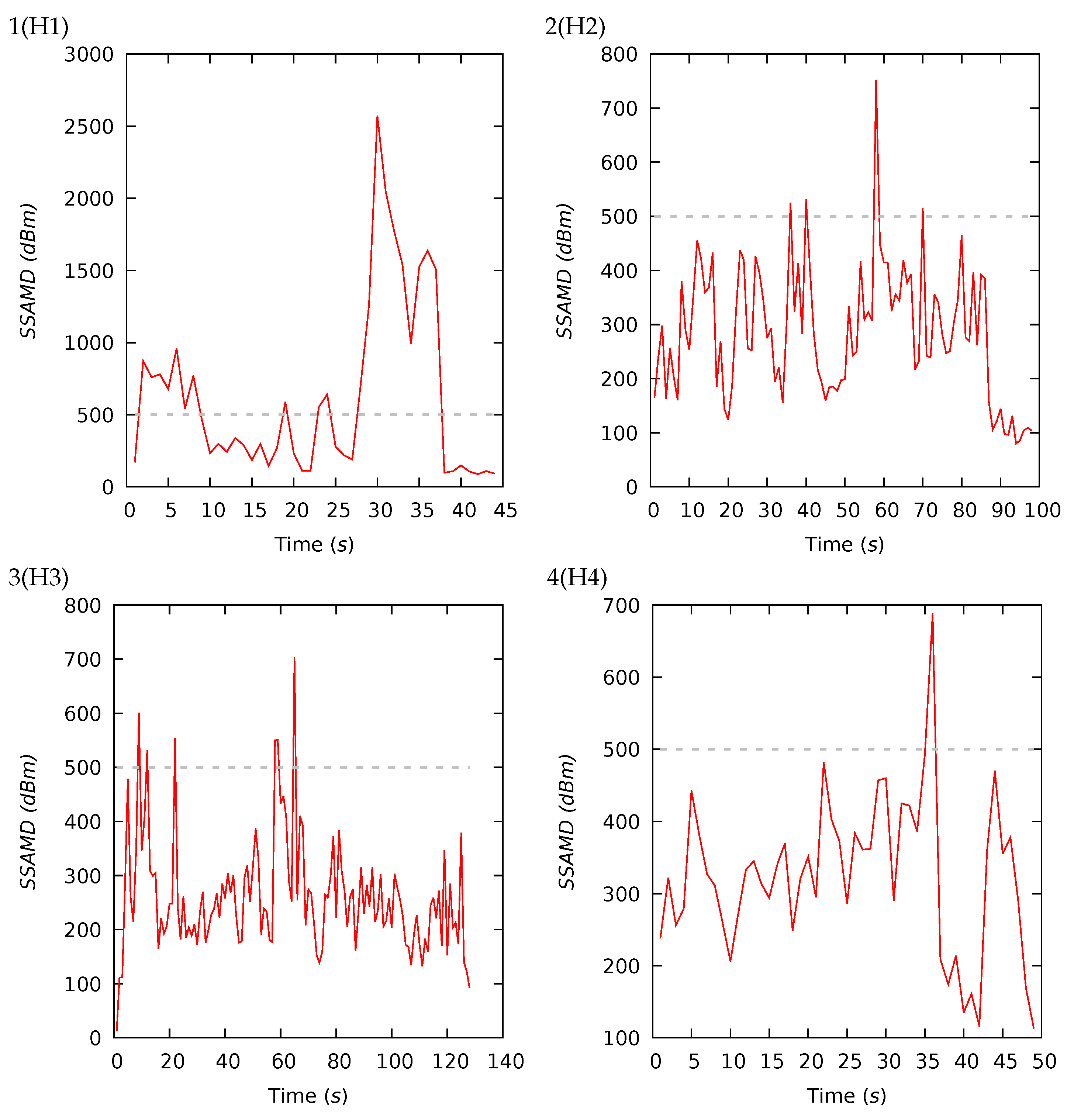
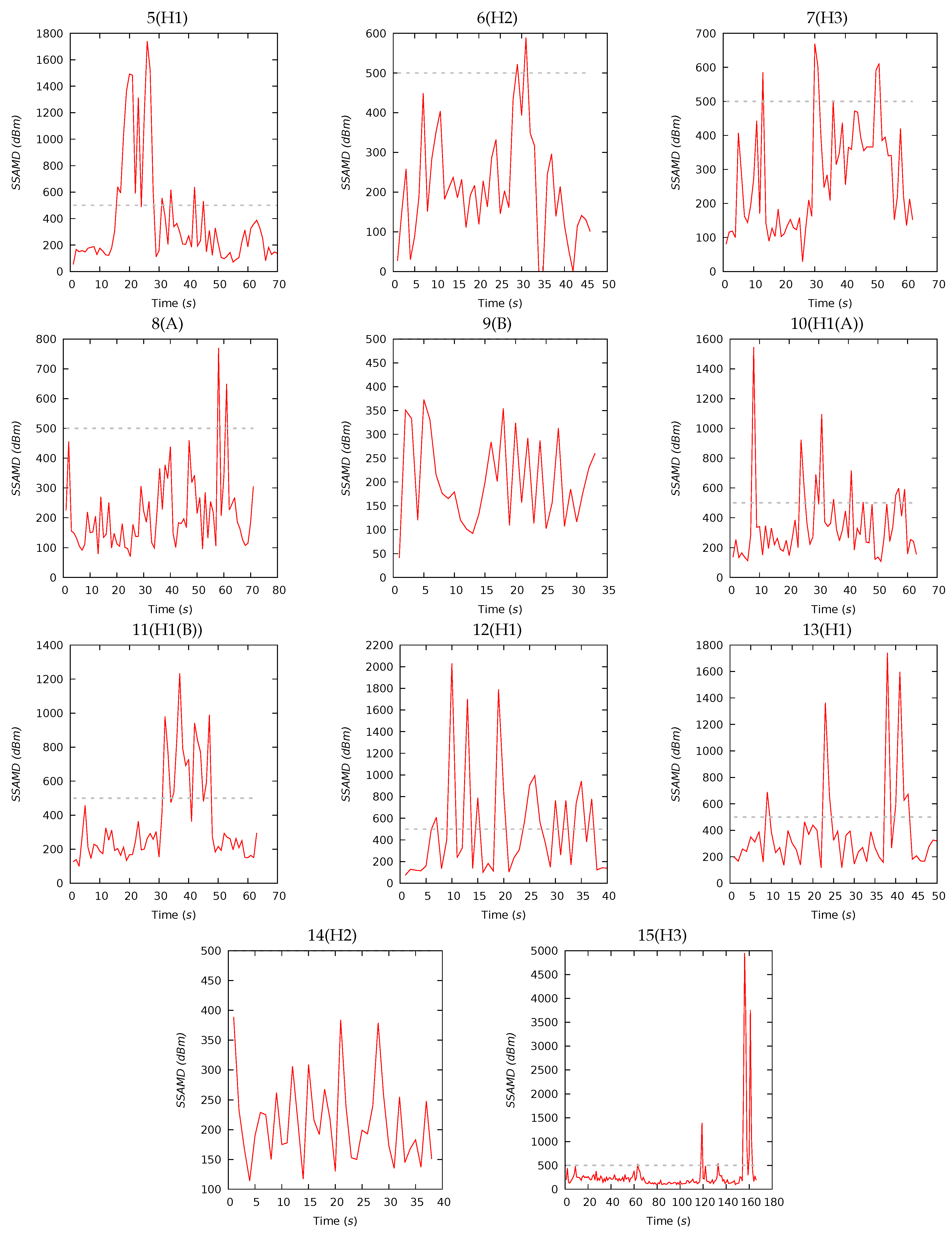
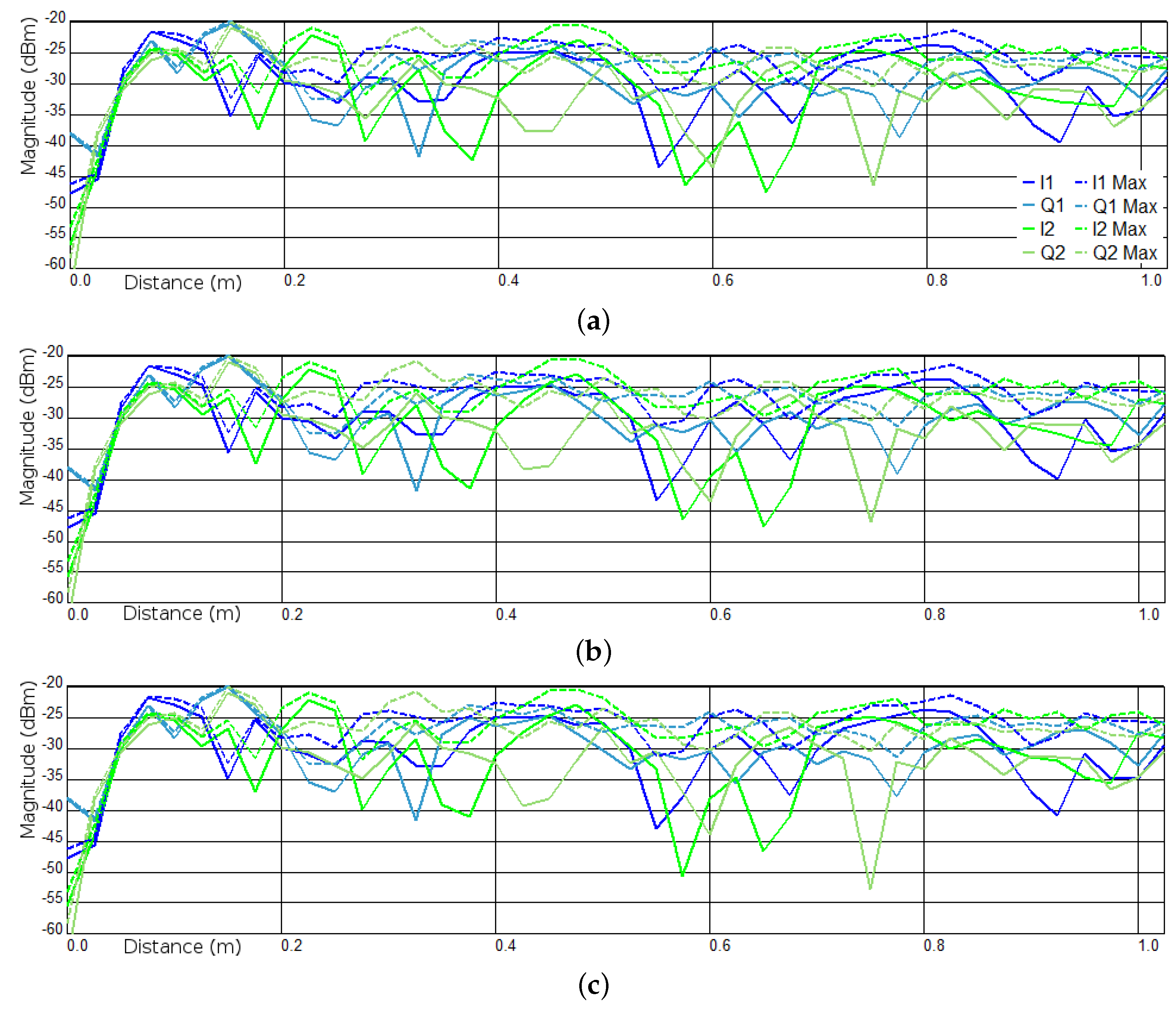
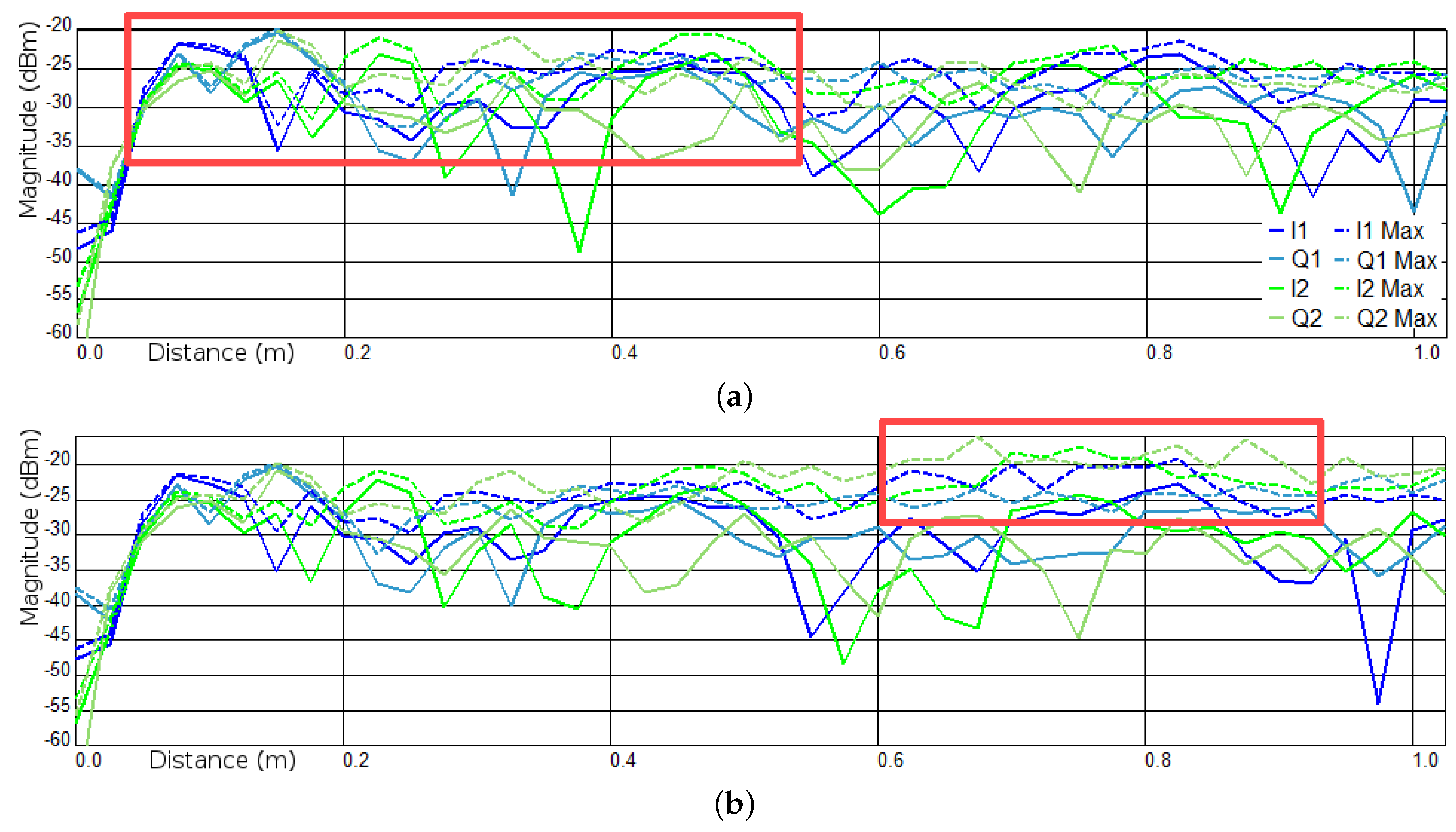
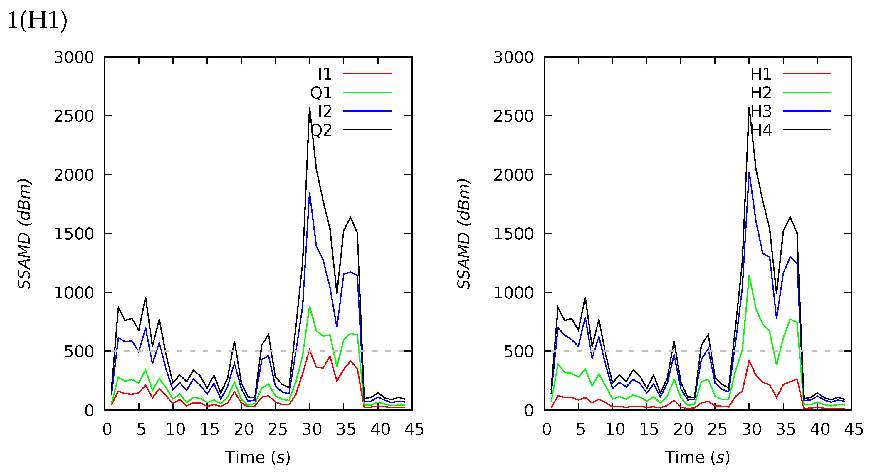
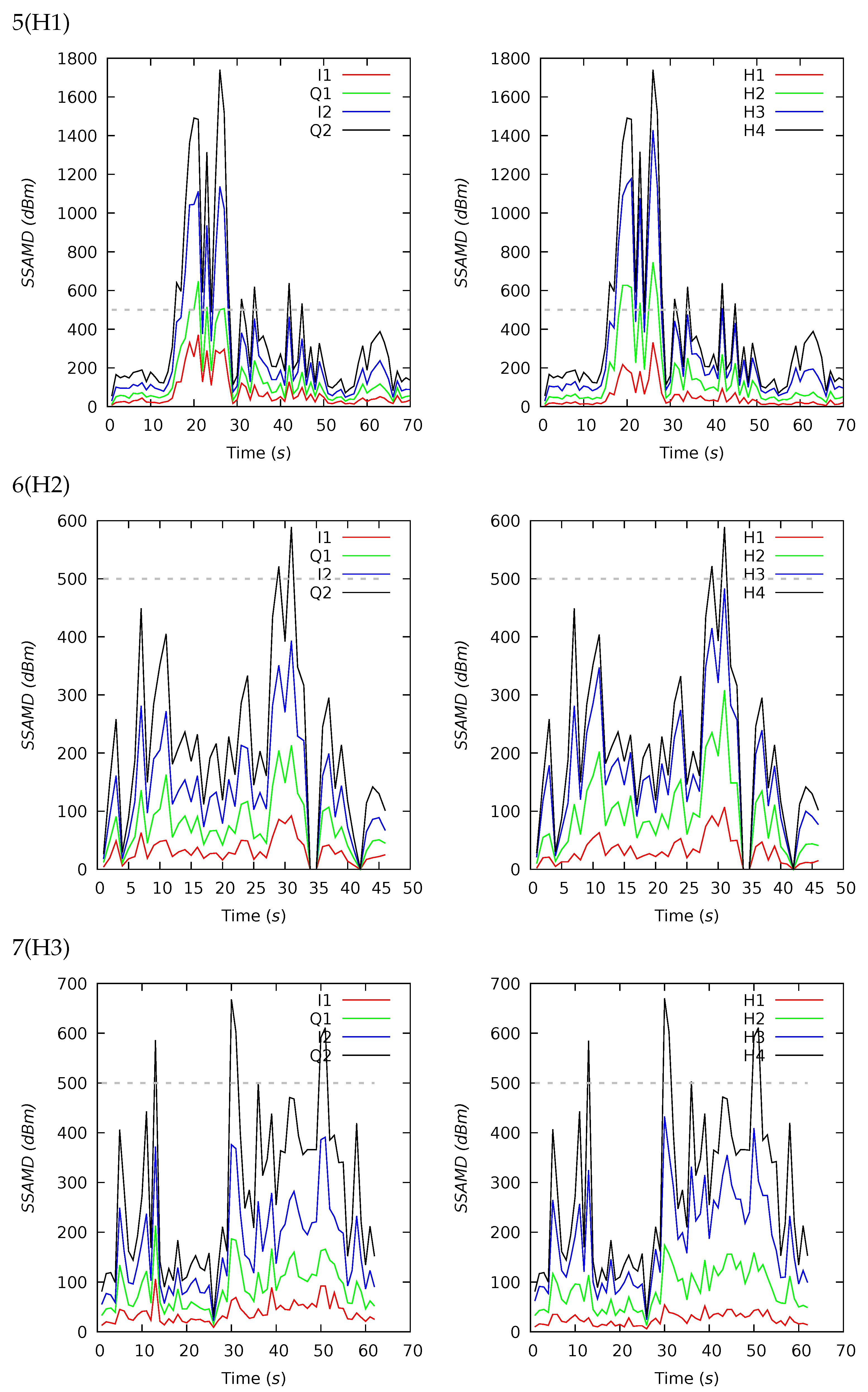
3.1. Experiments I and II—Presence Detection

Further, we discuss several charts reflecting the experiments’ flow and results. Figure 4 and Figure 5 plot S S A M D recorded during Experiments I and II. In the charts, the X and Y axes are for S S A M D and seconds correspondingly (both are integer values). All charts comprise the 500 S S A M D horizontal level; this is an empirical value. During the experiments, we have noticed that when there are no targets above the radar, S S A M D cannot reach 400 and can slightly exceed 400 when the diffuser covers it. Since the closest unreachable rounded level is 500, we use this value as a threshold for insect detection. This level indicates significant targets (i.e., values lower than 500 represent mainly noise).
Experiment I. Figure 4 shows the results of the first experiment. The experiment comprises four trials, each conducted at different height levels from H1 to H4. In 1(H1), the signal from the insect is quite strong. The presence is evident in the first ten seconds and from 28 to 37 s. Two weaker signals confirming the presence are recorded around the seconds 19 and 23. Here, 2(H2) detected the insect three times when it briefly passed the beam; 3(H3) recorded the presence five times. There is one signal that appears to be a false-negative before the first insect detection. It did not reach 500, but it is much stronger than any other noise levels. In 4(H4), there is only one case of reaching 500.
The experiment has proven that an insect can be detected at all altitude levels. We decided not to conduct the following experiments at the H4 height interval since it was difficult to operate with threads at such a distance from the radar.
Experiment II. Figure 5 shows the results of the second experiment. The upper column of the figure shows the results of trials 5–7 with a smaller insect, Sialis lutaria. As in the previous experiment, there was a much stronger signal (with maximal value 1740) on H1 and a relatively equal contribution of H2 and H3. In the 5(H1) chart, SSAMD significantly exceeded 500 from 15 to 27 seconds. There were also four smaller spikes from 30 to 50 s. The signal slightly exceeded 500 in two and three cases, not reaching 600 and 700 in the 6(H2) and 7(H3) charts, correspondingly. These trials prove the radar’s ability to detect smaller insects.
The following trials of the second experiment tested the radar with the diffuser. We shook the diffuser during the 8(A) trial. This can be observed around 60 s as two peaks of strength 600–800. The 9(B) trial was conducted without interrupting the diffuser, under completely calm conditions. The two following conclusions can be taken from these trials: first, the interruption of a diffuser causes the situation, which is very similar to an insect’s presence; second, in calm conditions, background noise makes frequent peaks slightly lower than 400. Findings in these and the previous trials allowed us to define the threshold of 500 for insect detection.
Charts of trials 10(H1(A)) and 11(H1(B)) show Sialis lutaria through the diffuser. Two acts carried out in different ways showed that such an insect produces local peaks of 800–1600. In trial 10(H1(A)), the insect passed the beam many times, while, in the 11(H1(B)) trial, it remained nearly statically around the radiation zone from 30 s to 50 s. Due to the higher dynamics of the former trial, the diversity of the peaks is higher there, while the latter showed the lower-diversity results.
The 12(H1) trial shows the results with a tiny fly. Interestingly, such a small insect could produce a S S A M D peak of around 2000. It is essential to mention that the insect was at the lowest possible height, almost touching the diffuser at 10 s (ca. 2000), 13 s (ca. 1700), and 19 s (ca. 1800). The other seven peaks were within 600 to 1000; they were produced from insects’ arbitrary positions within H1.
Trials 13(H1)–15(H3) show an interesting situation with the trials involving a cricket. Firstly, 13(H1) had a normal flow, with four registered peaks within 600 and 1800. In contrast, the next two trials were carried out with mistakes. Due to a mistake during 14(H2), the cricket never passed through the beam. As a result, the charts represent a situation without insects. Moreover, 15(H3) had another problem: an experimenter’s arm passed thorough the beam unintentionally. These mistakes allowed us to come to the following conclusions: first, the radiating zone has quite sharp edges and should be carefully defined before fieldwork; second, since even quick beam interruption generates such high S S A M D , the upper threshold can be defined to filter out larger possible targets (e.g., birds, bats, and shaking diffuser events). Careful observations let us define it as 3000, i.e., all peaks larger than 3000 should be considered suspicious and likely caused by larger (than insects) targets.

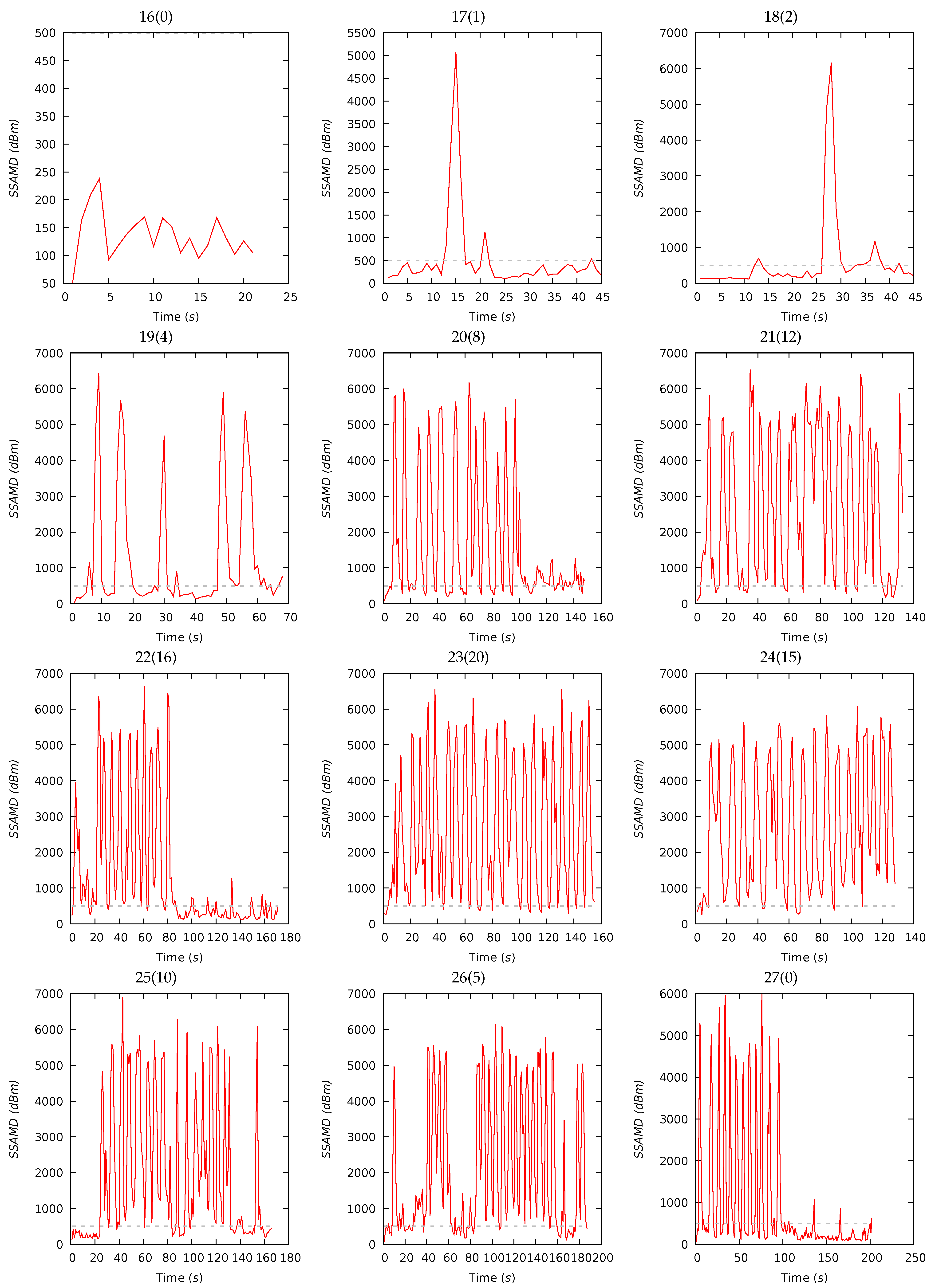
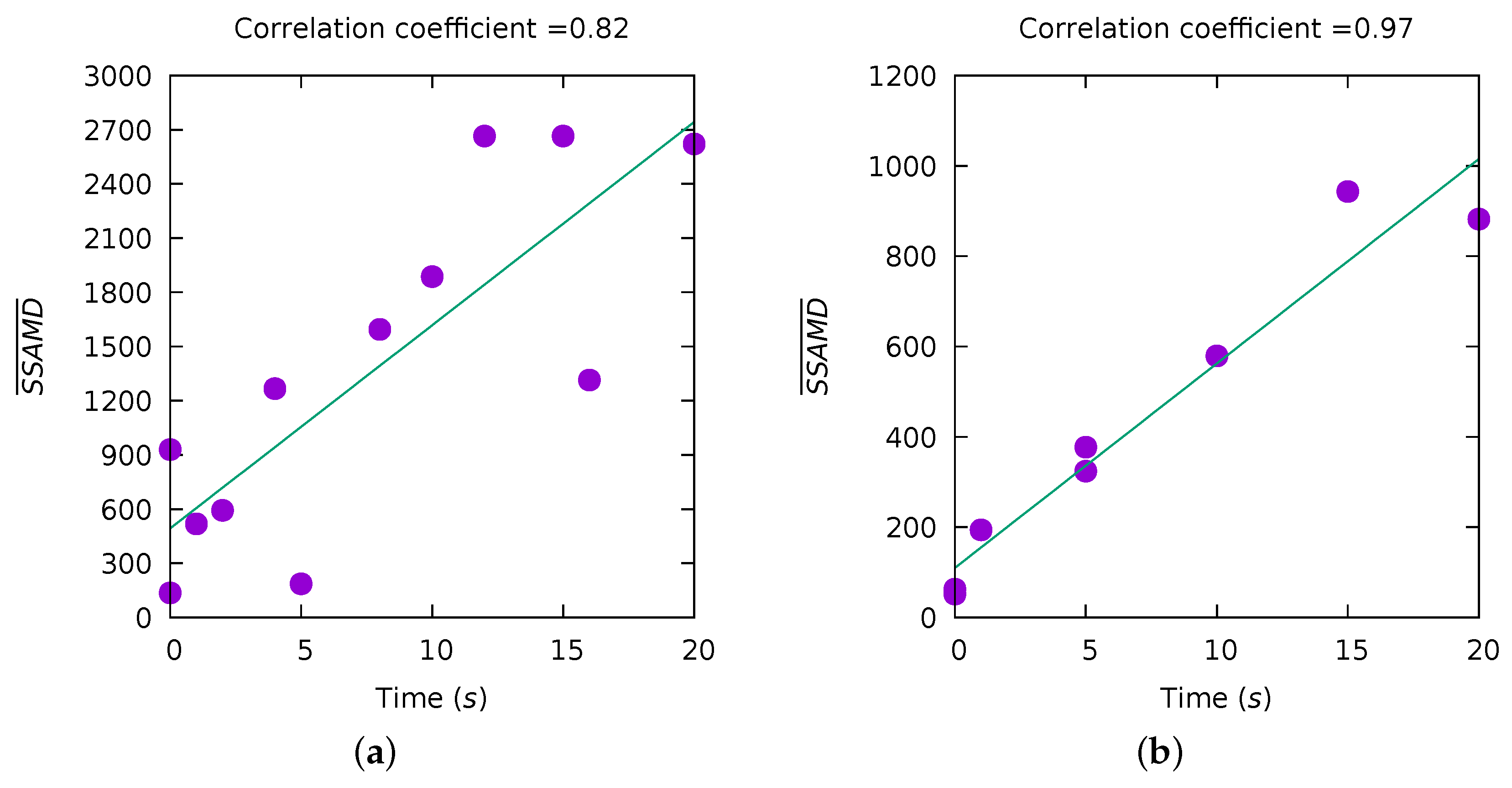
3.2. Experiment III—Biomass Estimation

Experiment III consists of two main steps: (a) trials 16(0)–27(0) depicted in Figure 6, (b) trials 28(0)–35(0) depicted in Figure 7. This experiment aims to disclose if it is possible to estimate the biomass using the considering radar setup. For every step, we use the various number of crickets provided in parentheses (i.e., 31(15) means trial number 31 with fifteen crickets); this applies for all trials of Experiment III. Since we will use a light trap to attract more insects in future fieldwork, we use the diffuser (light trap’s attractive screen) during this experiment. In addition to biomass estimation, the second step of Experiment III enables us to estimate ranges of S S A M D caused by many insects. This is important because the light trap will also attract many insects in field conditions.
As mentioned in Section 2.2, Experiment IIIa (Figure 6) was conducted in very uncertain conditions. We varied the duration of acts during the experiment and the number of shaking events from 0 to around 20. During acts 22(16) and 27(0), we even stopped shaking from the middle of acts to increase uncertainty. Events of shaking are distinguishable on the charts; the upper threshold of 3000 works well for recognizing shaking events here.
The left-hand side of Figure 8 shows a S S A M D ¯ for various numbers of insects. S S A M D ¯ values are in the range of ca. 100 to 2700 depending on the number of insects and number of shaking acts. As expected, the shaking effect can be distinguished due to the shape of the decreasing line after reaching the maximum. Since shaking acts affect all acts with various numbers of insects, it is automatically filtered out by the S S A M D ¯ parameter because the shaking contribution is relatively similar in multiple acts when the insects’ contribution varies, altering the mean value significantly.
Even in such ambiguous conditions, the correlation coefficient is 0.82. We do not expect such harsh conditions in the field because the developing insect radar setup will not be used during poor conditions with strong wind or precipitation (insects do not normally fly in such situations). Thus, we can conclude that biomass information can be obtained from such data. This can be achieved even with a diffuser and in complicated conditions.
Figure 7 shows the results obtained in a calm situation, or, in other words, insects behave quite naturally, crawling in the transparent plastic box without any intrusions. Before every act, we waited to allow the crickets to calm down. During the acts of Experiment IIIb, most of the crickets kept slowly crawling, seeking a place to hide. Only around a third of the box’s bottom surface was in the radiation zone. This means that crickets were able to leave this zone freely; their movement was quite chaotic, i.e., all parts of the box’s bottom were used with relatively equal probability.
These conditions reflected well in Figure 7. The transparent box decreased the background noise. As found earlier, the diffuser causes up to 400 S S A M D peaks, while the box created no more than 120. Furthermore, the figure illustrates that the insect led to wider spikes. This happened because a higher number of insects increases the probability of stronger reflection.
S S A M D ¯ variations of the acts of Experiment IIIb ranged from 50 to 850. Figure 8 plots these values and shows the high correlation of S S A M D ¯ and the biomass; the correlation coefficient is 0.97, which is much higher than in Experiment IIIa due to the lower uncertainty.

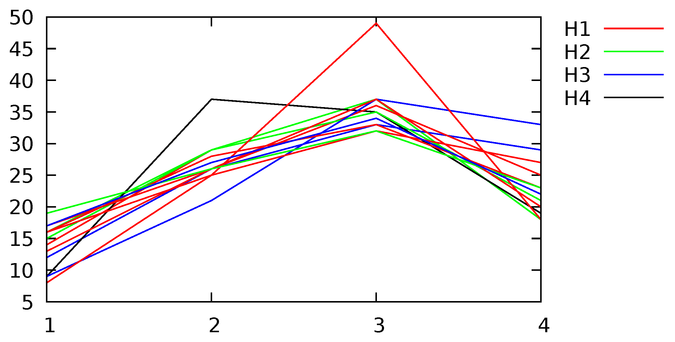
3.3. Resulting Table

Table 1 provides an overview of all experiments and their significant measurements. The table’s first column contains acts’ IDs (and short descriptions). For each act, we report its duration, statistics, and contributions of the height intervals and channels. Statistics comprise the mean, median, standard deviation, minimum, and maximal registered S S A M D . One can notice that the mean column represents S S A M D ¯ . Altitude and channel contributions are provided in percent. Moreover, the table shows overall statistics by column.
Altitude and channel contributions are provided in cells with a colored background. Colors represent the order of number using a blue-green-orange-red ramp, where blue and red are minimal and maximal values correspondingly. This allows the reader to interpret the contribution values easily. Regarding the height intervals’ contribution, one can notice that for all steps in Experiments I and II, H1 is a minimal contributor. Moreover, in most steps of all experiments, H3 is a maximal contributor. In contrast to this, the channels’ contribution is more diverse and random.
Overall, the statistics indicate that the shortest act duration is 21 s, while the longest is 202 s. The minimal S S A M D ¯ is 50, while the maximal is 2665; its average value is 710. As expected, the standard deviation is minimal for the empty transparent box (acts 28(0) and 35(0), values 19 and 20, correspondingly), while its maximal values are observed for Experiment IIIa. Interestingly, S S A M D reached zero only in two acts (6(H2) and 19(4)); their values usually are higher than 10. The maximal S S A M D (excluding Experiment IIIa) value, 2676, was predictably registered for act 32(20); its minimal value for acts with insects is 589 (6(H2)). These observations confirm the correctness of the defined lower and upper thresholds, 500 and 3000, correspondingly.
All channel and height interval magnitude contribution charts are provided in Appendix B. It is clear from Table 1 that the contribution of channels is relatively homogeneous. The average values are 20%, 20%, 30%, and 30% for Q1, I1, Q2, and I2, correspondingly. This means that either the Q or I channel can be deactivated (for instance, for energy consumption optimization) without significant information loss.

3.4. Low Possibility of Insect Range Estimation

Earlier, we showed the possibility of insect presence and biomass detection using the chosen FMCW radar device. Thus far, we have not found clear evidence of the range estimation possibility, but the question remains open. During the initial preliminary experiments, we noticed that the magnitudes’ dynamics differed with changing height intervals. We expected that this would be reflected on the resulting plots, but no clear evidence was registered.
We provide Figure 9 illustrating data from Table 1 regarding height interval contributions. Colored lines are for experiments conducted with an insect at a particular height interval (i.e., for acts comprising a height interval in their names). The plot shows the received magnitudes contribution (in percent) for all altitude levels. Let us consider specific height interval magnitudes’ contributions (see height contributions in Table 1) for trials with insects placed at height intervals H1, H2, and H3. We consider the following trials: H1—1(H1), 5(H1), 10(H1(A)), 11(H1(B)), 12(H1), and 13(H1); H2—2(H2), 6(H2), and 14(H2); H3—3(H3), 7(H3), and 15(H3). It is easy to confuse height interval magnitudes’ contributions (presented in the resulting table) and height intervals where insects were placed. The radar records magnitudes ordered by ranges (or distance from the radar); the ranges are estimated and, in our case, do not allow the actual target ranges to be calculated. We split these magnitudes using the earlier defined height intervals utilized for insect placing. The attached data [38] and software archive provide all concrete details (see Appendix D).
For the selected trials with known target height intervals, we calculated the average and median values for height interval magnitudes’ contributions. For H1 trials, H1, H2, H3, and H4 magnitudes’ average contributions (in %) are 14, 27, 37, and 22, correspondingly (median values are 14, 26, 37, 22); for H2 trials, H1, H2, H3, and H4 magnitudes’ average contributions (in %) are 17, 28, 35, and 21, correspondingly (median values are 17, 29, 35, and 21); for H3 trials, H1, H2, H3, and H4 magnitudes’ average contributions (in %) are 13, 25, 35, and 28, correspondingly (median values are 13, 26, 35, and 29). Therefore, in trials H1 and H2, magnitudes contribute similarly (i.e., from maximum to minimum—H3, H2, H4, and H1); meanwhile, in H3 trials, magnitudes’ average contributions from maximum to minimum are H3, H4, H2, and H1. This fact shows that higher objects cause magnitudes corresponding to higher ranges. In other words, it is potentially possible to obtain some rough insect range information. During the experiments, we also noticed differences in the noise fluctuation depending on the target height (see also Appendix A.2).
These observations allow us to suggest the potential possibility of approximate range detection. Of course, these findings are not well grounded (rather, they are preliminary thoughts). Further intensive experiments aiming at range estimation are required in order to clarify this. We suppose that there are higher chances of insect range detection for higher ranges of tens of meters.

4. Conclusions

This article continues the work presented in Reference [32]. In the mentioned review article, we demonstrate the fast-growing interest in compact FMCW radar systems. Furthermore, we have proposed a solution with a low-range radar set assembled with a light trap on a rover.
We propose a concrete novel technique for insect presence detection and biomass estimation using a compact low-range FMCW radar device. For this, we prepare a lab setup. Moreover, we propose a simple methodology for individual insect target investigation using cotton threads. Furthermore, we use a mass insect target investigation technique using either a light diffuser or a transparent plastic box. A series of experiments is conducted in very uncertain conditions. A novel proposed parameter allows us to process the obtained data, reduce the uncertainty, and present the results.
Initial unsuccessful tests showed that optimal radar parameters should be carefully defined empirically. We have refined the radar parameters during Experiment I, found an optimal means of connection, and defined the methodology for individual targets’ investigation. Next, we used various insect targets in Experiment II. It proved the chosen radar device’s applicability to detect even small insect targets at various height intervals from 0 to around 1 m. The final experiment, Experiment III, was devoted to biomass estimation using mass insect targets. Since, in Reference [32], we proposed to use a light diffuser, we used it in the first phase of the experiment with multiple cricket targets. To investigate mass targets in calm and clear conditions, we used a transparent plastic enclosure in the second phase of Experiment III. Every experiment comprised several trials; the trial was the part of the experiment devoted to recording the same target continuously.
We intentionally conducted the experiments in a way causing very uncertain collected data. Such data comprise a significant noise component, making them slightly closer to real field data. The noise contribution is so high that conventional tools for interpreting this radar’s data are useless. Therefore, we propose a novel parameter, the Sum of Sequential Absolute Magnitude Differences ( S S A M D ), for uncertainty reduction. This metric allows the aggregation of magnitude fluctuations within a defined time interval (we used a one-second interval) and can represent the results as a single float value. For continuously recorded data belonging to one act of the experiment, we propose to use the average of S S A M D values, or S S A M D ¯ . This metric enables us to compare trials regardless of their duration and conditions.
We carefully observed all trials of Experiments I and II and defined two S S A M D thresholds: 500 and 3000. S S A M D values lower than 500 are considered noise, values from 500 to 3000 indicate likely insect targets, and those over 3000 indicate larger targets (e.g., birds, bats, etc.). These experiments proved the radar’s insect presence detection ability. Experiment II, where we used mass cricket targets, was devoted to biomass estimation. In various conditions, from very uncertain to relatively structured, we radiated different numbers of targets in multiple trials. We have proven that S S A M D ¯ allows the estimation of biomass. The plots of S S A M D ¯ and insect numbers show the high correlation of these variables. In other words, the utilized setup can be used for insect biomass estimation.
In the next step, we will prepare an insect radar setup for extensive field trials based on the proposed solutions. As discussed in Reference [32], we will use a light trap; it will utilize a light diffuser similar to the one used in the experiments. It will be equipped with a camera to collect ground-truth information regarding attracted insect species. This will be a static setup; a rover will not be used in the next step.

Author Contributions

Conceptualization, J.B., A.N. and S.A.; methodology, A.N., J.B. and S.A.; software, A.N.; validation, J.B., A.N. and S.A.; formal analysis, A.N.; investigation, A.N.; resources, J.B. and S.A.; data curation, A.N.; writing—original draft preparation, A.N. and J.B.; writing—review and editing, A.N.; visualization, A.N.; supervision, J.B.; project administration, J.B.; funding acquisition, J.B. All authors have read and agreed to the published version of the manuscript.

Funding

This research was funded by the Hessian State Ministry for Higher Education, Research and the Arts, Germany, as part of the LOEWE priority project “Nature 4.0-Sensing Biodiversity”.

Institutional Review Board Statement

Not applicable.

Informed Consent Statement

Not applicable.

Data Availability Statement

The data presented in this study are openly available in Zenodo at https://zenodo.org/record/5035849, reference [38].

Conflicts of Interest

The authors declare no conflict of interest.

Appendix A. Experiment Details and Notes

Appendix A.1. Preliminary Tests

In preliminary tests, we tried to detect insects for the first time. The motivation for the first attempt was to check if we could detect real insects’ reflections in field conditions.
The idea was to install a light trap attracting insects. A camera (resided against the trap) took pictures of attracted insects to be used as ground-truth information. The trap radiated the light towards the camera. The radar was placed in between the light trap and camera. Thus, the majority of attracted insects should have passed the volume radiated by the radar.
We present our setup in Figure A1. In a garden, we installed a light trap illuminating intensive UV light. The camera and radar were installed as discussed. This setup was utilized for a few hours at night for the uninterrupted recording of radar data and the capturing of camera images.
Figure A1. Experiment 0: (a) the setup, (b) a sample photo with an insect.
Diversity 13 00452 g0a1
In order to detect insect targets, we analyzed the collected photos and radar data. We did not manage to distinguish insects from the noise. We have concluded that it was not appropriate to use the default configuration of the radar. Intensive lab experiments were required to define applicable configurations and setups; an optimal configuration is presented in Appendix C.

Appendix A.2. Experiment I

As found earlier, intensive lab tests are required to define an optimal radar configuration. For this, we devised a lab setup in which the radar was connected to a computer. Then, we captured several wild Phryganea grandis insects (see Figure A2, left).
Since the radar was not designed for insect detection, the software does not allow straightforward observations of insect targets. We have noticed that insects’ presence can be detected by the clutter dynamics in the following way: low dynamics indicate the absence of insects, while intensive dynamics indicate the presence of insect targets. Figure A3 shows frequency-domain data plots. The first two images represent no-insect conditions, while the last shows the reflectivity of an insect located in the H2 height interval. In general, fluctuations of the clutter are quite random, and the insect presence increases the fluctuations, but it does not allow us to observe an insect as a clear target.
Figure A2. Caught flying insects: (a) Phryganea grandis for Experiment I, (b) Sialis lutaria for Experiment II.
Diversity 13 00452 g0a2
Figure A3. Frequency domain data plots: (a,b) for no-insect conditions, (c) an insect in H2 (notice the higher amplitudes). Vertical axes are the magnitude levels in dBm; horizontal axes are the distances in meters.
Diversity 13 00452 g0a3
Figure A4 plots time moments when insects were placed at different height intervals. One can notice that (a) has larger maximum values in the low-altitude part than the higher-altitude part, while the opposite is true for (b); red boxes highlight these results.
Figure A4. Frequency domain data plots with an insect in H1 (a) and H2 (b). Vertical axes are the magnitude levels in dBm; horizontal axes are the distances in meters.
Diversity 13 00452 g0a4
In addition to frequency-domain plots, history plots allow observation of the insects. Figure A5 depicts an H3 insect reflection (appearing between 108 and 109 s). As with the frequency-domain data plots, we can distinguish the presence, but the reflection has quite a random character. All other plot types provided by the utilized radar software do not allow us to observe insects convincingly. For this, new data processing and visualization are required to work with such data. At the end of the section, we propose a solution for this.
Figure A5. History plot showing an insect (highlighted by a red ellipse) in H3 (108–109 s).
Diversity 13 00452 g0a5
The first experiment has proven that insects can be detected with low-range radar. However, it has also indicated the necessity for further evaluations in different conditions. First of all, other insects should be observed. Second of all, we need to verify the reflectivity through a cover material. Since we intend to use the device in forest field conditions, the radar must be covered so as to be protected from the rain. Moreover, we plan to use the radar with a light trap to attract insects. To address both requirements, we can use a regular bowl-shaped light diffuser. In the following experiment, we consider these questions.

Appendix A.3. Experiment II

As discussed earlier, another experiment with different insects and a light diffuser is needed. For this experiment, we caught some insects. For the cover, we used a standard acrylic light diffuser. As in the previous step, we used threads for holding insects above the radar device.
A Sialis lutaria insect (see Figure A6) is smaller than the insect in Experiment I. We radiated the insect at three altitude levels.
Figure A6. An experiment with Sialis lutaria.
Diversity 13 00452 g0a6
In addition, we worked with an average-sized house cricket at the same altitude levels. It is much more challenging to hold crickets. They are much more robust and active than the other used insects. They use their strong legs to release themselves from the thread. As in the previous attempts, the charts reflected the insect in a similar way.
Earlier, we used quite large insects (body length of ca. 1.5–2.5 cm). Next, we chose to use much smaller objects. For this, we illuminated a small house fly and a woodlouse (crustacean). Both had a size of around 0.5 cm (see Figure A7). It was difficult to observe them at the H2 and H3 height intervals. Both were clearly visible at the H1 level.
Figure A7. (a) Musca domestica (a small house fly), (b) Armadillidium vulgare (a small woodlouse; crustacean).
Diversity 13 00452 g0a7
Next, it was necessary to verify that insects could be detected through the diffuser. For this, we covered the device with the diffuser (see Figure A8) and hung the Phryganea grandis insect above the setup on the H1 level. This means that we can use the device in real conditions with a cover illuminating the light from inside to attract nocturnal insects. Furthermore, we can place the electronics under the cover to protect the setup from precipitation.
Figure A8. Light diffuser covering radar.
Diversity 13 00452 g0a8

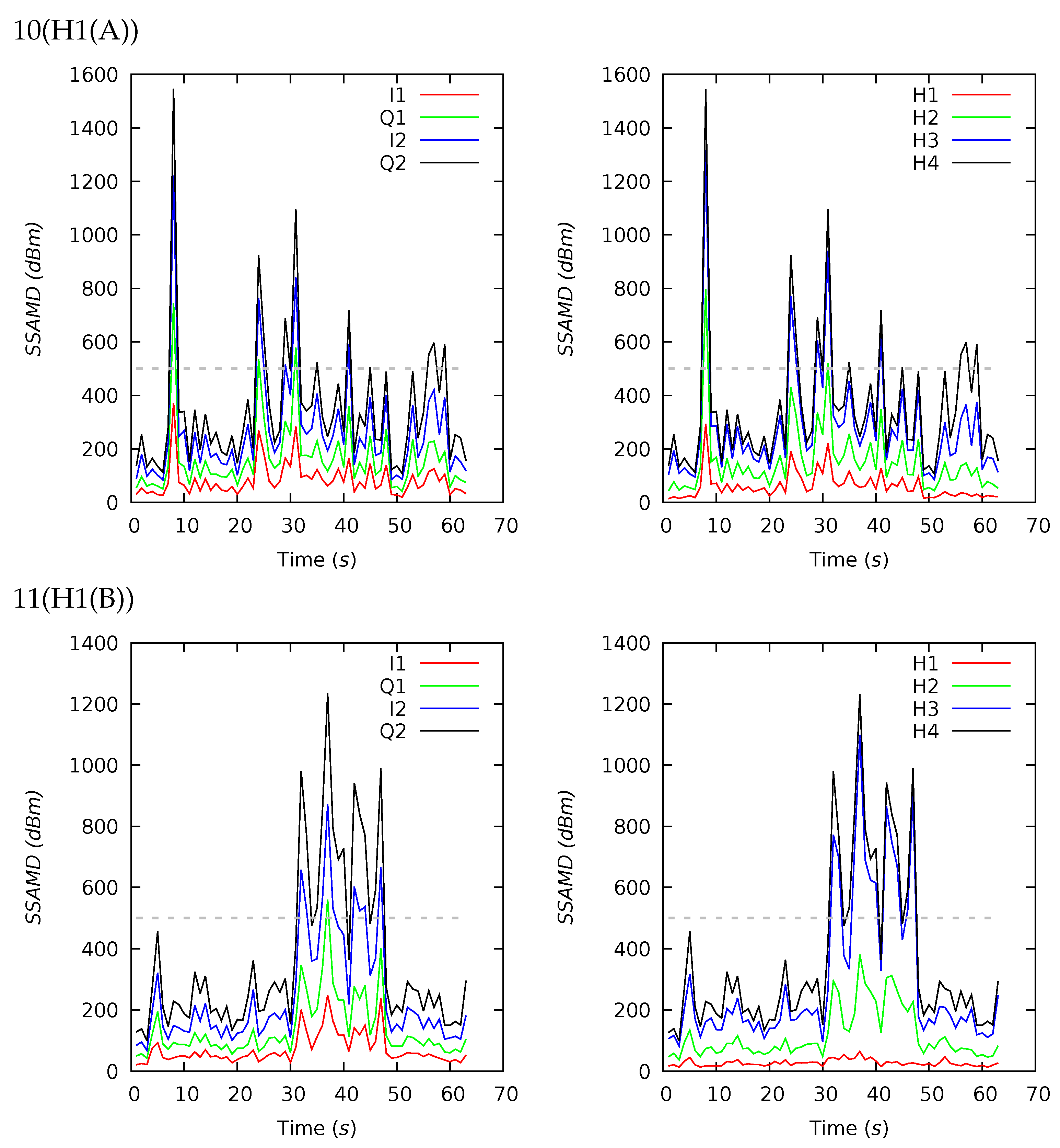
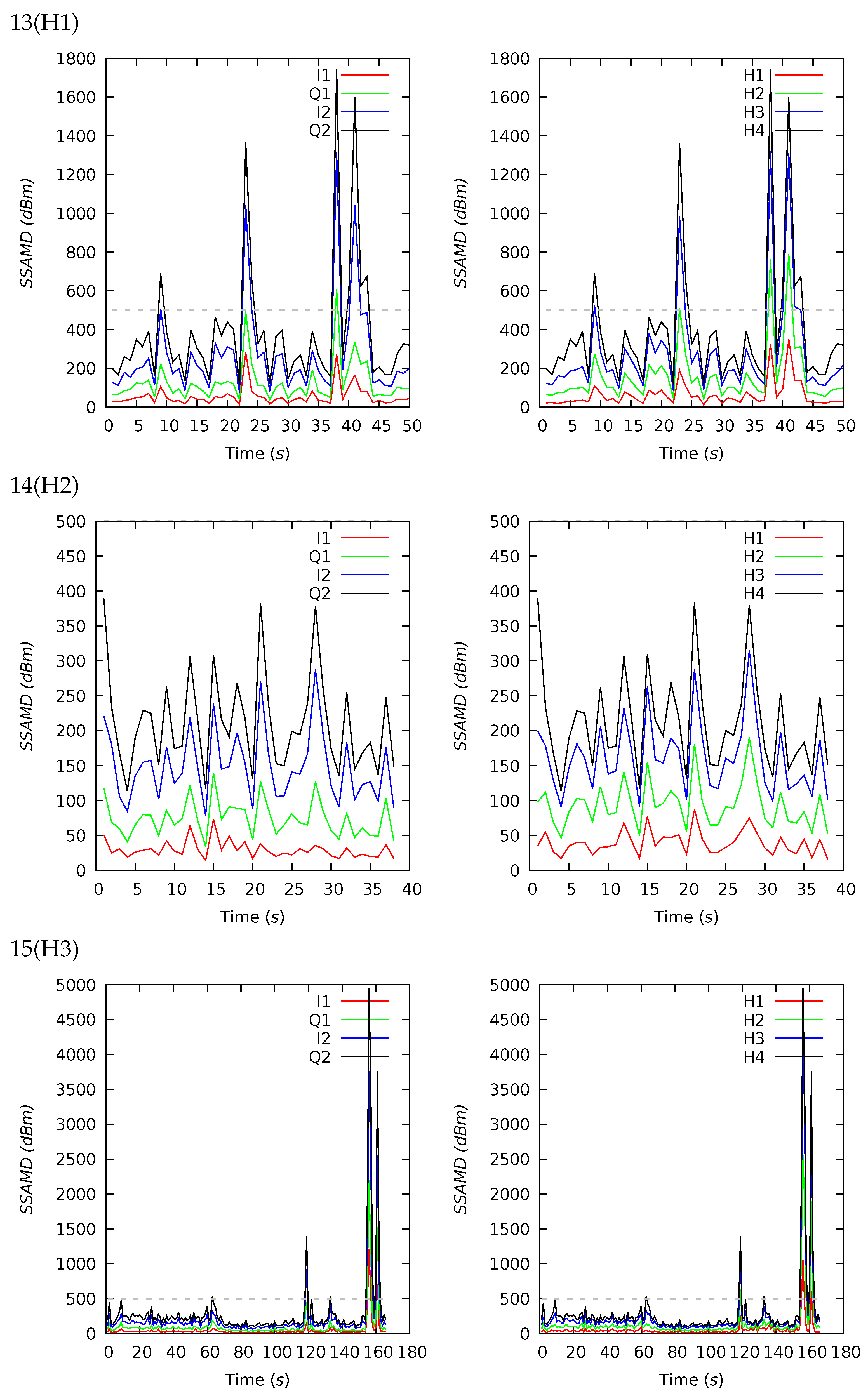
Appendix B. Channel and Height Level Contributions

Two types of charts are provided from left to right: (left) four-line chart broken down into channels’ contributions using red, green, blue, and black colors for I1, Q1, I2, and Q2 channels, correspondingly, (right) four-line chart broken down into altitudes’ contributions using red, green, blue, and black colors for H1, H2, H3, and H4 height intervals, correspondingly.
Figure A9, Figure A10, Figure A11, Figure A12 and Figure A13 show channels’ and height interval magnitudes’ contributions to the trials of the first and second experiments. In 1(H1) (Figure A9), the channels’ contribution is relatively equal in “non-insect” intervals, while it differs in “insect” intervals. In the interval from 28 to 37 s, the shape of the curve is mainly formed by I2, while I1 and Q2 contribute much less. Despite the distinguished facts, one can notice that the channels’ contribution is distributed relatively randomly. There is an interesting situation with height intervals’ contributions. Regardless of expectations, H1 contributes the least (14%), while H3 gives 37%. These facts confirm our supposition that it will be difficult to calculate targets’ ranges. H2 and H3 mainly form the curve’s shape. In 2(H2), the channels’ contributions are relatively similar. In trials 5–7 (Figure A10), as earlier, I2 and H3 mainly form the shape of the curve. In 13(H1) (Figure A13), major signal contributors are I2 and H3.
Figure A9. Experiment I, Phryganea grandis 1–4 (H1–H4).
Diversity 13 00452 g0a9aDiversity 13 00452 g0a9b
Figure A10. Experiment II, Sialis lutaria 5–7 (H1–H3).
Diversity 13 00452 ga10
Figure A11. Experiment II, Sialis lutaria through the diffuser (10–11).
Diversity 13 00452 ga11
Figure A12. Experiment II, a small fly through the diffuser (12(H1)).
Diversity 13 00452 ga12
Figure A13. Experiment II, a single cricket through the diffuser (13–15 (H1–H3)).
Diversity 13 00452 ga13

Appendix C. Radar Software Installation and Configuration

Radar software was designed for the Windows operating system. In future work, we wish to run the radar on Unix-like systems. In particular, Raspberry Pi is our target computer. For the lab experiments, we have been able to run the original software delivered with the radar. To operate it on Debian-like systems (we use the GNU/Linux Debian Buster operational system), one should execute the following commands for the dependencies installation:
  • sudo apt-get install wine64 winetricks \
  • winetricks corefonts d3dx9_36 vcrun2005 vcrun2008 vcrun2010 \
  • winhttp
Now, the delivered software can be installed from the flash drive. One should execute the following command to run the installed software:
  • WINEPREFIX=~/.wine/drive_c/Program\ Files/SenTool_60GHz/ \
  • wine \
  • /home/$USER/.wine/drive_c/Program\ Files/SenTool_60GHz/StartApp.exe
Moreover, the network should be appropriately configured. Only the following configuration of Network Manager Applet of Mate Desktop Environment allowed us to work with the radar smoothly without any problems: (Ethernet Tab) MTU: 32; (IPv4 Settings Tab) Address: 192.168.0.1, Netmask: 16, Gateway: 192.168.0.2, DNS servers: 192.168.0.2.
In the radar software, we use the following IP address and port number for the connection: IP 192.168.0.2, Port 1024. Moreover, we use the following measuring parameters: start frequency 58 GHz, stop frequency 64 GHz, ramp time 1 ms, zero pad factor 1, time interval 50 ms, maximal distance 1 m, and measure type FMCW Up-Ramp. All receive channels are enabled. Frontend power, power saving, and normalization modes are activated. The one-meter maximal range provides good perception; a larger range would be unnecessary since single insect targets can be detected up to approximately 1 m. For all the following experiments, we use the presented configuration.

Appendix D. Resulting Data and Data Processing Software

Reference [38] provides the collected data, data processing software, and resulting datasets. It consists of three files, R a w D a t a . z i p , r a d a r . t c l , and R e s u l t s . z i p . R a w D a t a . z i p , comprising the collected data organized by experiment and trial directories. Each trial directory comprises F D (frequency-domain) directories containing the main text data files; T D (time-domain) directories are not utilized in the present work. Some trial directories also comprise PNG files with screenshots of the radar software charts taken during the experiments.
r a d a r . t c l is a script developed for R a w D a t a . z i p data processing. The script does not have specific dependencies; thus, it should work in every system with Tcl 8.6+ and GNUPlot5 installed; it was tested only in a Unix environment. The U S A G E section of the script provides instructions for running it. The following Bash commands automate data processing and generate the resulting datasets and charts (they are also provided in r a d a r . t c l ):
  • for cur in $(find /home/username/RadarLab/RawData \
  • -type d -name FD)
  • do; tclsh radar.tcl \$cur /tmp/Results \
  • ‘echo \$cur|xargs dirname|xargs dirname|sed \’
  • ‘s/. *RawData//g; s/\///g’|sed ‘s/\///g’; done
The resulting dataset archive ( R e s u l t s . z i p ) includes PDF charts and trials’ S S A M D calculations (TXT files). A file r a d a r s t a t s . t x t comprises aggregated statistics provided in Table 1.

References

  1. Hochkirch, A. The insect crisis we can’t ignore. Nature 2016, 539, 141. [Google Scholar] [CrossRef] [Green Version]
  2. Hallmann, C.A.; Sorg, M.; Jongejans, E.; Siepel, H.; Hofland, N.; Schwan, H.; Stenmans, W.; Müller, A.; Sumser, H.; Hörren, T.; et al. More than 75 percent decline over 27 years in total flying insect biomass in protected areas. PLoS ONE 2017, 12, e0185809. [Google Scholar] [CrossRef] [Green Version]
  3. McGrath, M. Global Insect Decline may See ‘Plague of Pests’. 2019. Available online: https://www.bbc.com/news/science-environment-47198576 (accessed on 20 December 2020).
  4. Didham, R.K.; Basset, Y.; Collins, C.M.; Leather, S.R.; Littlewood, N.A.; Menz, M.H.M.; Müller, J.; Packer, L.; Saunders, M.E.; Schönrogge, K.; et al. Interpreting insect declines: Seven challenges and a way forward. Insect Conserv. Divers. 2020, 13, 103–114. [Google Scholar] [CrossRef] [Green Version]
  5. Petrovskii, S.; Petrovskaya, N.; Bearup, D. Multiscale approach to pest insect monitoring: Random walks, pattern formation, synchronization, and networks. Phys. Life Rev. 2014, 11, 467–525. [Google Scholar] [CrossRef]
  6. Gressitt, J.L.; Gressitt, M.K. An improved Malaise trap. Pac. Insects 1962, 4, 87–90. Available online: http://hbs.bishopmuseum.org/pi/pdf/4(1)-87.pdf (accessed on 20 September 2021).
  7. Southwood, E. Ecological Methods with Particular Reference to the Study of Insect Populations; Barnes and Noble: New York, NY, USA, 1966; 409p. [Google Scholar]
  8. Gunstream, S.E.; Chew, R.M. A Comparison of Mosquito Collection by Malaise and Miniature Light Traps1. J. Med. Entomol. 1967, 4, 495–496. [Google Scholar] [CrossRef]
  9. Owen, D.F. Species diversity and seasonal abundance in tropical Sphingidae (Lepidoptera). Proc. R. Entomol. Soc. Lond. Ser. A Gen. Entomol. 1969, 44, 162–168. [Google Scholar] [CrossRef]
  10. Shimoda, M.; Honda, K. Insect reactions to light and its applications to pest management. Appl. Entomol. Zool. 2013, 48, 413–421. [Google Scholar] [CrossRef] [Green Version]
  11. Yao, Q.; Lv, J.; Liu, Q.J.; Diao, G.Q.; Yang, B.J.; Chen, H.M.; Tang, J. An Insect Imaging System to Automate Rice Light-Trap Pest Identification. J. Integr. Agric. 2012, 11, 978–985. [Google Scholar] [CrossRef]
  12. White, P.J.T.; Glover, K.; Stewart, J.; Rice, A. The Technical and Performance Characteristics of a Low-Cost, Simply Constructed, Black Light Moth Trap. J. Insect Sci. 2016, 16, 25. [Google Scholar] [CrossRef] [Green Version]
  13. Bjerge, K.; Nielsen, J.B.; Videbæk Sepstrup, M.; Helsing-Nielsen, F.; Høye, T.T. An Automated Light Trap to Monitor Moths (Lepidoptera) Using Computer Vision-Based Tracking and Deep Learning. Sensors 2021, 21, 343. [Google Scholar] [CrossRef] [PubMed]
  14. Ruczyński, I.; Hałat, Z.; Zegarek, M.; Borowik, T.; Dechmann, D.K.N. Camera transects as a method to monitor high temporal and spatial ephemerality of flying nocturnal insects. Methods Ecol. Evol. 2019, 11, 294–302. [Google Scholar] [CrossRef]
  15. Pádua, L.; Adão, T.; Sousa, A.; Peres, E.; Sousa, J.J. Individual Grapevine Analysis in a Multi-Temporal Context Using UAV-Based Multi-Sensor Imagery. Remote Sens. 2020, 12, 139. [Google Scholar] [CrossRef] [Green Version]
  16. Song, B.; Park, K. Verification of Accuracy of Unmanned Aerial Vehicle (UAV) Land Surface Temperature Images Using In-Situ Data. Remote Sens. 2020, 12, 288. [Google Scholar] [CrossRef] [Green Version]
  17. Crawford, A. Radar reflections in the lower atmosphere. Proc. Inst. Radio Eng. 1949, 37, 404–405. [Google Scholar]
  18. Riley, J. Radar as an Aid to the Study of Insect Flight. In A Handbook on Biotelemetry and Radio Tracking; Pergamon Press: Oxford, UK, 1980; pp. 131–140. [Google Scholar] [CrossRef]
  19. Vaughn, C.R. Birds and insects as radar targets: A review. Proc. IEEE 1985, 73, 205–227. [Google Scholar] [CrossRef]
  20. Rainey, R.C. Observation of Desert Locust Swarms by Radar. Nature 1955, 175, 77. [Google Scholar] [CrossRef]
  21. Hao, Z.; Drake, V.A.; Sidhu, L.; Taylor, J.R. Locust displacing winds in eastern Australia reassessed with observations from an insect monitoring radar. Int. J. Biometeorol. 2017, 61, 2073–2084. [Google Scholar] [CrossRef]
  22. Smith, A.; Riley, J. Signal processing in a novel radar system for monitoring insect migration. Comput. Electron. Agric. 1996, 15, 267–278. [Google Scholar] [CrossRef]
  23. Chapman, J.; Smith, A.; Woiwod, I.; Reynolds, D.; Riley, J. Development of vertical-looking radar technology for monitoring insect migration. Comput. Electron. Agric. 2002, 35, 95–110. [Google Scholar] [CrossRef]
  24. Chapman, J.W.; Reynolds, D.R.; Smith, A.D. Vertical-Looking Radar: A New Tool for Monitoring High-Altitude Insect Migration. BioScience 2003, 53, 503–511. [Google Scholar] [CrossRef] [Green Version]
  25. Mascanzoni, D.; Wallin, H. The harmonic radar: A new method of tracing insects in the field. Ecol. Entomol. 1986, 11, 387–390. [Google Scholar] [CrossRef]
  26. Riley, J.; Smith, A. Design considerations for an harmonic radar to investigate the flight of insects at low altitude. Comput. Electron. Agric. 2002, 35, 151–169. [Google Scholar] [CrossRef]
  27. Colpitts, B.; Boiteau, G. Harmonic Radar Transceiver Design: Miniature Tags for Insect Tracking. IEEE Trans. Antennas Propag. 2004, 52, 2825–2832. [Google Scholar] [CrossRef]
  28. Psychoudakis, D.; Moulder, W.; Chen, C.; Zhu, H.; Volakis, J.L. A Portable Low-Power Harmonic Radar System and Conformal Tag for Insect Tracking. IEEE Antennas Wirel. Propag. Lett. 2008, 7, 444–447. [Google Scholar] [CrossRef]
  29. Drake, V.; Reynolds, D. Radar Entomology: Observing Insect Flight and Migration; CAB International: Wallingford, UK, 2012. [Google Scholar]
  30. Chapman, J.W.; Drake, V.A.; Reynolds, D.R. Recent Insights from Radar Studies of Insect Flight. Annu. Rev. Entomol. 2011, 56, 337–356. [Google Scholar] [CrossRef] [PubMed] [Green Version]
  31. Shamoun-Baranes, J.; Nilsson, C.; Bauer, S.; Chapman, J. Taking radar aeroecology into the 21st century. Ecography 2019, 42, 847–851. [Google Scholar] [CrossRef]
  32. Noskov, A.; Bendix, J.; Friess, N. A Review of Insect Monitoring Approaches with Special Reference to Radar Techniques. Sensors 2021, 21, 1474. [Google Scholar] [CrossRef] [PubMed]
  33. Jansson, S.; Malmqvist, E.; Brydegaard, M.; Akesson, S.; Rydell, J. A Scheimpflug lidar used to observe insect swarming at a wind turbine. Ecol. Indic. 2020, 117, 106578. [Google Scholar] [CrossRef]
  34. Rankin, G.A.; Bui, L.Q.; Tirkel, A.Z.; Le Marshall, N. Radar imaging: Conventional and MIMO. In Proceedings of the 2012 Fourth International Conference on Communications and Electronics (ICCE), Hue, Vietnam, 1–3 August 2012; pp. 171–176. [Google Scholar] [CrossRef]
  35. IMST. IMST Sentire Radar Module 24 GHz sR-1200 Series: User Manual; Version 1.3; IMST GmbH: Kamp-Lintfort, Germany, 2017; Available online: https://imst.de/ (accessed on 20 September 2021).
  36. Kirkhorn, J. Introduction to IQ-Demodulation of RF-Data; IFBT, NTNU: Trondheim, Norway, 1999. [Google Scholar]
  37. Mendelson, G. All You Need to Know about Power over Ethernet (PoE) and the IEEE 802.3 af Standard; PowerDsine Ltd.: Hod HaSharon, Israel, 2004. [Google Scholar]
  38. Noskov, A. Low-Range FMCW Insect Radar—Lab Experiments Data, Results, and Data Processing Software. 2021. Available online: https://doi.org/10.5281/zenodo.5035849 (accessed on 20 September 2021).
Figure 1. IMST sentire FMCW 60 GHz Radar Module: (a) photo; (b) a corresponding generalized block diagram of a CW/FMCW radar system with transmitter and receiver channels and I/Q demodulator. The diagram consists of the following elements: the signal source for the generation of a (frequency-modulated) signal, transmitter antenna (Tx), receiver antennas (Rx), mixers for the generation of the intermediate frequency, digital sampling unit; also, the device comprises other elements: couplers, filters, amplifiers, phase shifters. Antennas reside on the top of the device.
Diversity 13 00452 g001
Figure 2. Phryganea grandis: (a)—tied with a thread, (b)—placed above the radar.
Diversity 13 00452 g002
Figure 3. A few Acheta domesticus (house cricket) insects in: (a) a flipped light diffuser, (b) transparent packing box.
Diversity 13 00452 g003
Figure 4. Experiment I. Phryganea grandis, various height intervals.
Diversity 13 00452 g004
Figure 5. Experiments II. Sialis lutaria, no targets, Acheta domesticus, and Musca domestica. Various height intervals. Trials 8–15 were carried out with the light diffuser.
Diversity 13 00452 g005
Figure 6. Crickets in the flipped diffuser (shaking acts).
Diversity 13 00452 g006
Figure 7. Crickets in the plastic box (no shaking).
Diversity 13 00452 g007
Figure 8. Biomass estimation. (a)—Experiment IIIa; (b)—Experiment IIIb.
Diversity 13 00452 g008
Figure 9. Contribution of magnitudes belonging to different distances to S S A M D for targets located at a specific height interval: X-axis—height interval of contributing magnitudes, Y-axis—the contribution in percent, colored lines—targets located at a specific height interval.
Diversity 13 00452 g009
Table 1. Experiments: resulting statistics. Desc—description; Dur—duration; StDev—standard deviation. Blue-green-orange-red cell background colors represent numbers from minimal to maximal values, correspondingly.
ID (Desc)Dur (s)SSAMD’s Statistics (dBm)Contribution (%)Contribution (%)
MeanMedianStDevMinMaxH1H2H3H4Q1I1Q2I2
Experiment I (Phryganea grandis)
1(H1)446263196088825731429372015222835
2(H2)98286279121807521629371817213032
3(H3)128261244105137041226332920263123
4(H4)49325327110113688937351918233227
Experiment II
Sialis lutaria:
5(H1)703842074015417401326362517193232
6(H2)4621219013605891529352120153530
7(H3)6227623415729669921373318143929
Diffuser (no insects):
8(A)7121318312670770717344218144028
9(B)332031799341373919343819153729
Sialis lutaria through the diffuser:
10(H1(A))6335026924610815451726372022242430
11(H1(B))633592582641001233825491818203230
Small fly through the diffuser:
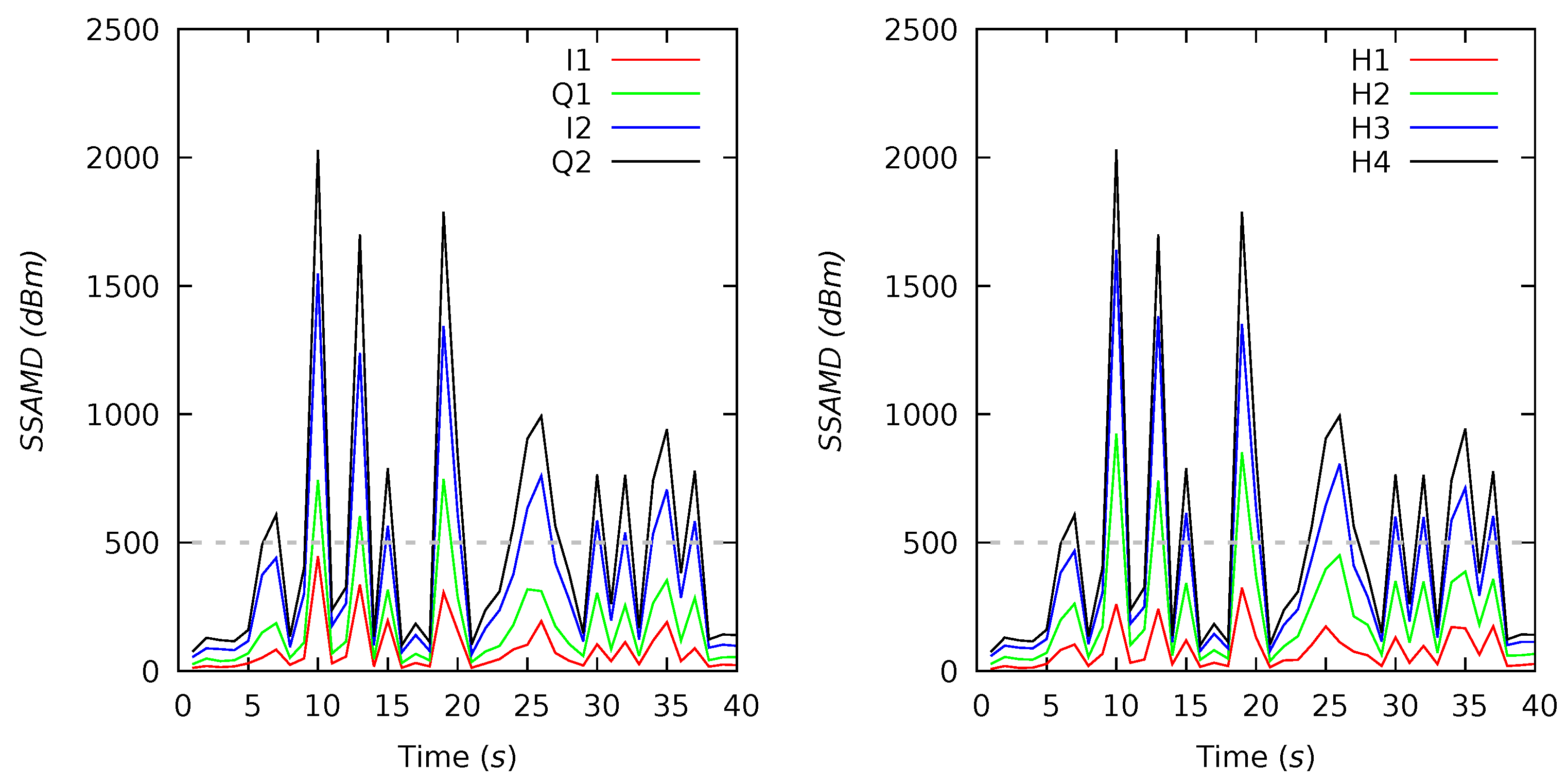
12(H1)404973184817520301628332319172638
Single cricket through the diffuser:
13(H1)5038528933811717421625322718142939
14(H2)38212196711143891926322321143035
15(H3)1663031895659849491727342219153135
Experiment III
Experiment IIIa—Crickets in the diffuser (shaking):
16(0)2113613142502381528381923153032
17(1)4551828488210350641627391820183131
18(2)45593275113111561621428401823242528
19(4)6812673961752064292030351521232729
20(8)148159568117847861732030351521242728
21(12)1332665250920709265332230331523252626
22(16)1711314527172211866342229341523242726
23(20)15526212028195725265562130341522242628
24(15)12826652145185624760782130351422242628
25(10)1661887865197513568962128341722252627
26(5)1872033103519097661562029351623252626
27(0)20293027314855859932127361622242727
Experiment IIIb—Crickets in the box (at rest):
28(0)37636319261171723411925212628
29(5)363241403795013401827381723204017
30(10)325795154296918951433371621213127
31(15)3094383845516217821430401617223625
32(20)3488274564810226761730391416203529
33(5)313771304145412081230382017203924
34(1)38194110209529161826411514143933
35(0)3552502091132621302321142441
Overall Statistics by Column
Mean747104696677926681627372020203030
Median463772734017617401628361820213029
StDev5474356769256244144473455
Min215250190113717301314141917
Max20226652509207025268962637494225264042
Publisher’s Note: MDPI stays neutral with regard to jurisdictional claims in published maps and institutional affiliations.

