Article

Assessing the Genetic Diversity of Ilex guayusa Loes., a Medicinal Plant from the Ecuadorian Amazon

by
Maria P. Erazo-Garcia
1,
Juan José Guadalupe
1,
Jennifer K. Rowntree
2,
Pamela Borja-Serrano
1,
Nina Espinosa de los Monteros-Silva
1 and
Maria de Lourdes Torres
1,*
1
Laboratorio de Biotecnología Vegetal, Colegio de Ciencias Biológicas y Ambientales, Universidad San Francisco de Quito USFQ, Campus Cumbayá, P.O. Box 17-1200-841, Quito 170901, Ecuador
2
Department of Natural Sciences, Ecology and Environment Research Centre, Manchester Metropolitan University, Manchester M1 5GD, UK
*
Author to whom correspondence should be addressed.
Diversity 2021, 13(5), 182; https://doi.org/10.3390/d13050182
Submission received: 25 March 2021 / Revised: 20 April 2021 / Accepted: 24 April 2021 / Published: 28 April 2021

Abstract

:
Ilex guayusa Loes. is a shrub native to the Neotropics, traditionally consumed as an infusion. Despite its cultural value and extensive use, genetic research remains scarce. This study examined the genetic and clonal diversity of guayusa in three different Ecuadorian Amazon regions using 17 species-specific SSR markers. The results obtained suggest a moderately low degree of genetic diversity (He = 0.396). Among the 88 samples studied, 71 unique multilocus genotypes (MLGs) were identified, demonstrating a high genotypic diversity. A Discriminant Analysis of Principal Components (DAPC) revealed the existence of two genetic clusters. We propose that a model of isolation-by-environment (IBE) could explain the genetic differentiation between these clusters, with the main variables shaping the population’s genetic structure being temperature seasonality (SD × 100) (Bio 4) and isothermality ×100 (Bio 3). Nonetheless, we cannot dismiss the possibility that human activities could also impact the genetic diversity and distribution of this species. This study gives a first glance at the genetic diversity of I. guayusa in the Ecuadorian Amazon. It could assist in developing successful conservation and breeding programs, which could promote the economic growth of local communities and reinforce the value of ancestral knowledge.

1. Introduction

Ilex guayusa Loes. (Aquifoliaceae) is a shrub or a small tree [1] native to the Neotropics [2,3], distributed along the Amazon region of Colombia, Ecuador, Peru, and Bolivia [1,2,3,4,5,6]. It is commonly used to prepare tea-like infusions similar to other Amazonian beverages such as yerba mate (I. paraguariensis A. St.-Hil) and guaraná (Paullinia cupana Kunth) [6]. An important attribute of guayusa tea is its high caffeine content and a very palatable flavor without the bitterness often perceived in common tea (Camellia sinensis (L.) Kuntze) [7,8]. It grows in altitudes ranging from 200 to 2000 m.a.s.l. [6,9], and Ecuador appears to be the main center for its cultivation, especially towards the eastern Andean slopes and the adjacent Amazonian piedmont [4,9,10,11]. Growing as part of secondary forests, guayusa proliferates on sandy-loam soils with acidic pH, and in humid and semi-dark environments [2]. Extensive use of this species by humans throughout its range of distribution strongly suggests some degree of domestication [3]. At present, its reproduction is only known to occur asexually through human propagation of basal shoots and hardwood stem cuttings [2,11]. Years of vegetative propagation and selection by humans have likely induced the loss of guayusa flowering capability [12]. According to the Global Biodiversity Information Facility (GBIF) database (accessed on 24 June 2020), the most recent preserved fertile specimen was collected in Peru in 2004. In Ecuador, the last fertile collected specimen is from 1985 [13]. The common absence of fruiting or flowering material is probably the cause of its poor representation in the world’s herbaria collections [10,12], positioning guayusa as one of the most poorly understood species of the Ilex L. genus [7].
The earliest report of human use of this species can be traced back to 500 A.D. according to archaeological material found in Bolivia [4]. However, the first report of guayusa leaves being extensively consumed as a decoction dates back to 1683 among different Amazonian groups, mainly Shuar, Achuar, and Kichwas [1,4,5,6,8,10]. It is primarily used as a purgative and a tonic to allay fatigue and hunger, and it has also been used to improve digestion, treat venereal diseases, overcome sterility, increase libido, cure dysentery, flu, amenorrhoea, and stomach aches, and to avoid insect and snake bites [3,4,5]. Several other medicinal properties have been attributed to guayusa tea, such as antibacterial, antifungal, antiviral, expectorant, anti-inflammatory, diuretic, emetic, narcotic, hypnotic, and anesthetic [2,3,5,9,10,12]. The ancestral knowledge associated with this plant species has been passed down through generations among indigenous groups. Guayusa is considered a “magical” plant by local groups [4,10] and has even been included in burial ceremonies [5]. Guayusa tea also has a ritual significance and is consumed during indigenous activities such as the preparation of curare and ayahuasca [4,12], the Women’s Tobacco Ceremony, and the Tsantsa Feast [3,4].
Indigenous communities commonly cultivate guayusa in small horticultural plots known as chacras principally for self-consumption [3,4] and commercialization [9,11]. Recently, guayusa has been sold as a non-Camellia tea alternative, achieving popularity in the United States and China [6]. Seeking international markets for this product and enhancing sustainable development through food tourism [9] could provide a great economic opportunity for the country and the Amazonian communities while reinforcing the value of traditional agroforestry [11].
Several species of the Ilex genus, such as I. paraguariensis [14,15,16], I. chinensis Sims [17], I. integra Thunb. [18], and I. aquifolium L. [19], among others [20,21,22], have been widely studied in terms of their genetic diversity and phytochemical composition [23,24]. In the case of guayusa, most research has focused on exploring its chemical properties and ethnobotanical uses [3,6,9], while information on genetics and cultivation history remains scarce [25]. Given that guayusa’s primary strategy for reproduction is asexual and human-mediated, establishing its genetic status represents an interesting case study. Commonly, vegetative reproduction has been associated with reduced levels of clonal and genetic diversity [26,27,28]. However, some studies suggest otherwise, stating that plant species with diminished or even absent sexual reproduction can show equivalent levels of genetic diversity to those that reproduce sexually [26,27]. In order to understand which of these is the case of guayusa, in the present study we performed a preliminary assessment of the genetic diversity and population structure of 88 guayusa individuals from the Ecuadorian Amazon using 17 Simple Sequence Repeats (SSR) markers specific for I. guayusa. Having information of this species at the genetic level could contribute to establish conservation strategies and develop breeding programs [14] for the sustainable use of this agroforestry resource in a fragile and highly biodiverse region [25].

2. Materials and Methods

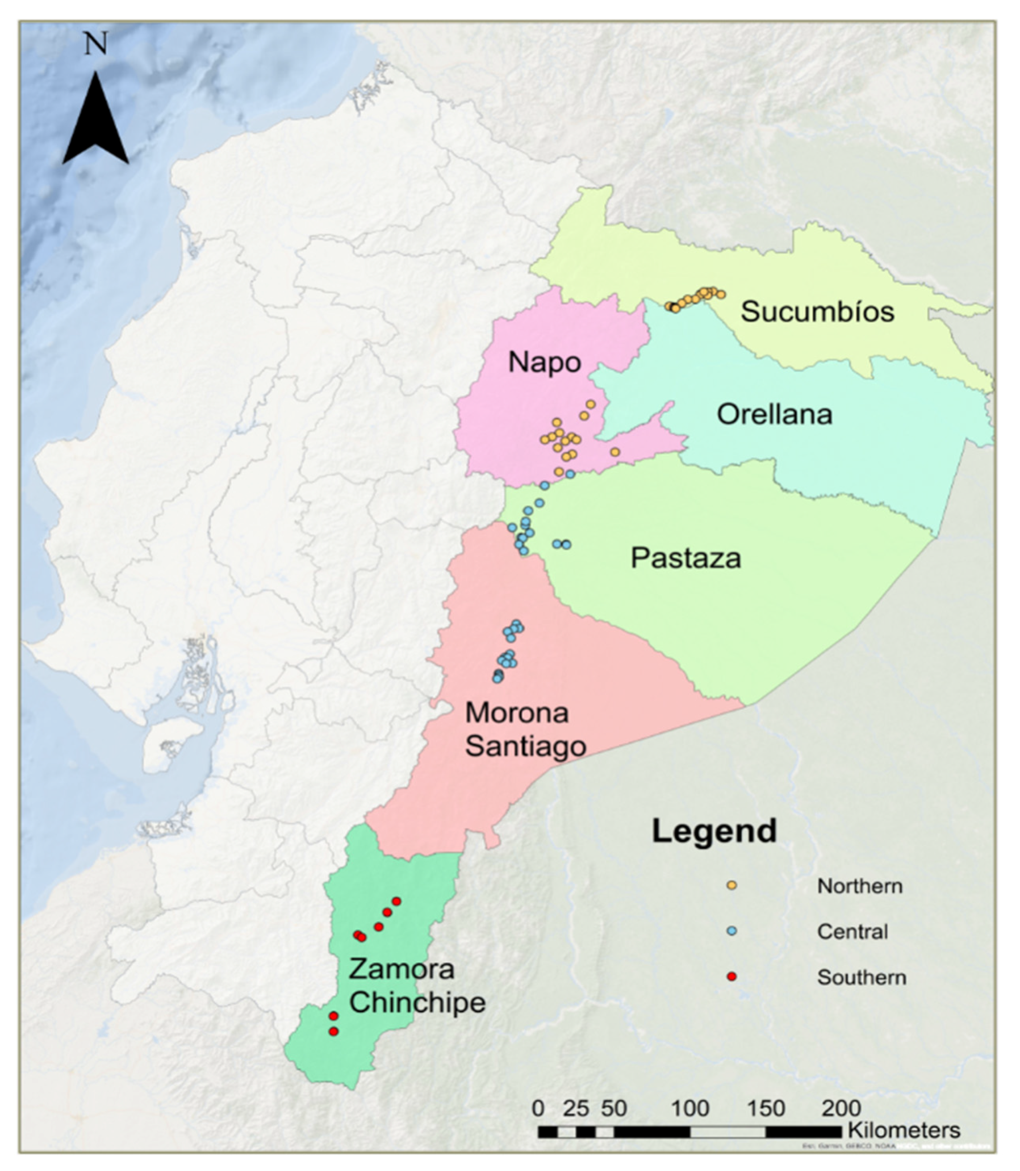
2.1. Sample Collection

Ilex guayusa samples were collected at selected locations throughout the six Amazon provinces of Ecuador (Sucumbíos, Napo, Orellana, Pastaza, Morona Santiago, and Zamora Chinchipe). These locations included small cultivation sites near highways, villages, and forest patches that were found with the guidance of local inhabitants. The samples were selected with a distance of at least 100 m between individuals to avoid resampling of the same genet. Samples consisted of 3–5 young and healthy leaves located at the apical zones of lower branches. They were immediately preserved at −20 °C inside Ziploc bags after their collection. A total of 88 samples were included in this study (Table S1). Good coverage of the sampling area was achieved by collecting 15 guayusa individuals from each province, except for Zamora Chinchipe, where only 13 samples were obtained. Collection sites were georeferenced using a Garmin E-Trex Legend HCx GPS (Garmin International Inc., Olathe, KS, USA), and a map with the coordinates (Figure 1) was drawn using the ArcGIS Desktop v.10.8 tool (Environmental Systems Research Institute, Redlands, CA, USA) [29].

2.2. Genomic DNA Isolation

Total genomic DNA was isolated using a modified CTAB-activated charcoal protocol described by Križman et al. (2006) [30] and an inhibitor-free isolation protocol for recalcitrant plants described by Rezadoost et al. (2016) [31]. Briefly, 1.5 cm2 of a leaf was finely ground in a mortar with liquid nitrogen and homogenized with 1 mL of extraction buffer: 100 mM Tris-HCl pH 8, 2 M NaCl, 20 mM EDTA pH 8, 2% (w/v) CTAB, 1% (w/v) PVP (MW 10,000), 0.5% (w/v) activated charcoal, and 1% (v/v) β-mercaptoethanol; the last two components were suspended right before use [30]. The mixture was transferred into a microcentrifuge tube and incubated at 55 °C for 30 min with frequent agitation. Samples were centrifuged at 16,000× g for 10 min, and the supernatant was transferred to a new tube. One volume of chloroform-isoamyl alcohol (24:1) was added to each tube and vortexed thoroughly. Samples were then centrifuged at 16,000× g for 10 min, and the chloroform-isoamyl alcohol step was repeated. After subsequent centrifugation, the supernatant was transferred to a new tube, and ½ volume of Buffer 2 was added: 50 mM Tris–HCl, 2 M guanidine thiocyanate, 0.2% (v/v) β-mercaptoethanol, and 0.2 mg/mL proteinase K; the last two components were suspended right before use [31]. Tubes were incubated at 40 °C for 15 min, and one half of total volume 4 M NaCl was added. Tubes were placed on ice for 5 min, and then 300 µL of isopropanol was mixed by inversion. Incubation took place at room temperature for at least 1 h. Tubes were centrifuged at 9000× g for 20 min, and pellets were washed with 500 µL of wash buffer (15 mM ammonium acetate in 75% (v/v) ethanol) [30]. Pellets were air-dried for 15 min, and DNA was suspended in 30 µL of ultra-pure distilled water. DNA quality and concentration were assessed using a NanoDrop 2000 Spectrophotometer (Thermo Scientific, Wilmington, DE, USA). Samples were diluted to a final concentration of 30 to 60 ng/µL.

2.3. Development of SSR Markers for Ilex guayusa

SSR markers were developed at the University of Manchester Genomics Facility using the Galaxy-based bioinformatics pipeline for Illumina next-generation sequencing data [32]. Briefly, DNA was fragmented on a sonicator and size-selected before sequencing. The Illumina MiSeq platform was used to sequence a single individual of I. guayusa with the shotgun 2 × 250 paired-end sequencing methodology (Nextera DNA Preparation Kit, Illumina, San Diego, CA USA) and using 0.33 of a flow cell. After sequencing, data quality was assessed using FastQC [33], and reads were filtered and trimmed using Trimmomatic [34].
Microsatellite loci were located and identified using PAL finder v.0.02 [35]. The configuration was set to search for sequences with a minimum of eight repeated units for each locus, with motifs varying between two and six nucleotides. The function Pal_filter [32] was used to remove imperfect, interrupted repeats, loci without primers, and loci where the primer sequence had occurred in more than one read. The functions PANDASeq and Pal_filter [32] were used to assemble paired-end reads. Primer3 software was used for oligo design [36,37]. Primer design was optimized for use with Platinum Taq DNA polymerase (Invitrogen, Carlsbad, CA, USA) with an optimal Tm of 62 °C and a maximum difference of 3 °C among primers.
A total of 14,903,079 raw sequence reads were produced, with none flagged as poor quality. Sequence length ranged from 50 to 300 bp with a reported GC content of 37%. After screening, a total of 328 primer pairs were obtained; 13 SSRs had motifs of 3 bp and the rest consisted of 2 bp motifs. From the total, 17 SSRs were selected as candidates for our study (Table S2). The melting temperature (Tm) of the primer sets ranged from 58 to 63 °C, and primer length varied from 18 to 25 bp. Locus-specific forward primers were synthesized, including a universal tail (Tail A) complementary to universal primers fluorescently labeled with VIC, 6-FAM, NED, or PET [38].

2.4. Sample Preparation and Genotyping

For each set of primers, the optimal annealing temperature was adjusted to perform further PCR amplification. PCR products were amplified and fluorescently labeled using a three-primer system protocol described by Blacket et al. (2012) [38]. PCR reactions were carried in a total volume of 30 µL containing 1 U of Platinum Taq polymerase (Invitrogen, Carlsbad, CA, USA), 1× PCR Buffer, 3 mM MgCl2, 1 mg/mL BSA, 0.2 mM dNTPs, 0.5 µM universal fluorescent primer, 0.15 µM forward primer, 0.5 µM reverse primer and 30 ng of DNA template. Cycling conditions consisted of an initial denaturation of 94 °C for 15 min, followed by 45 cycles of 94 °C for 30 s, 90 s at the optimal annealing temperature, 72 °C for 60 s, and a final elongation step at 72 °C for 5 min. Successful amplification was checked by running an electrophoresis of the PCR products in a 1.5% (w/w) agarose gel stained with SYBR Safe (Invitrogen, Carlsbad, CA, USA). Labeled PCR products were genotyped by Macrogen Inc. (Seoul, Korea) in an ABI 3730xl DNA Analyzer (Applied Biosystems, Foster City, CA, USA) using 500LIZ as the size standard. Genotyping results were read using GeneMarker v.2.4.0 (Softgenetics, State College, PA, USA) [39].

2.5. Data Analysis

2.5.1. Genetic Diversity

For the analyses, we divided the Ecuadorian Amazon area into three regions: Northern, Central, and Southern, considering the latitudinal range where the samples were collected, from −0.00913 to −4.64852 latitudes. Each region covered a latitudinal extension equivalent to 1.75 decimal degrees. Multilocus genotypes (MLGs) were assigned to the individuals using GenoDive v.1.2 to identify potential clones [40]. Average Bruvo’s genetic distances [41] across all loci were used as input for GenoDive. These were calculated using the poppr package available for R v.1.3.959 [42,43] and transformed (range from 0 to 100). A clonal threshold of 2 was used according to the parameters for threshold selection suggested by Meirmans and Van Tienderen [40]. Pairs of individuals with a genetic distance below the threshold shared the same MLG and were therefore considered clones. To avoid a biased estimation of genetic diversity and population structure, analyses were conducted using clone correction, which is a method of data censorship [44]. In this way, clones were censored at the region level, and only one individual per MLG was represented in the dataset.
A genotype accumulation curve was calculated using the poppr R package [42] with 10,000 permutations to determine the loci’s resolution power to discriminate between genotypes. The probability of observing a particular MLG in an individual was calculated with the same package using the formula Pcgen = (∏pi)2h, where pi is the frequency for each allele observed in the MLG and h is the number of heterozygous loci. Then, (Pcgen)n−1 was obtained, where n is the number of times the genotype was observed in the population. These statistics were calculated to assess the probability that the same MLGs were assigned by chance between individuals [45].
Indexes of clonal diversity were calculated in GenoDive. The total number of alleles (A), expected heterozygosity (He), observed heterozygosity (Ho), and F-statistics were obtained using the hierfstat R package [46]. The adegenet R package [47] was used to evaluate the inbreeding coefficients’ distribution as an indicator of the proportion of inbreeding. Private alleles (PA) were determined with the poppr R package [42], and the mean allelic richness (AR) standardized to the minimum sample size (N = 13) through rarefaction was calculated with the diveRsity R package [48]. The polymorphic information content (PIC) for each primer was determined with the polysat R package [49], and null allele frequencies for all loci were calculated with FreeNA [50]. The Hardy–Weinberg equilibrium was tested for all loci using the pegas R package [51].

2.5.2. Population Structure

To test genetic differentiation among and within regions, an Analysis of Molecular Variance (AMOVA) was performed using GenAlex v.6.5 with 9999 permutations [52]. The hierfstat R package [46] was used to calculate pairwise FST between regions. In species with clonal or mixed reproduction (sexual and asexual), model-free clustering methods are recommended to infer population structure [53,54]. For this reason, a DAPC was performed with the adegenet R package [47]. To determine the optimal value of genetic clusters (K), values of between 1 and 10 were assayed by calculating the Akaike information criterion (AIC) and the Kullback Information Criterion (KIC) statistics [55]. The number of PCs retained for DAPC was determined by a mean a-score optimization and stratified cross-validation.
A Principal Coordinates Analysis (PCoA) was performed with the ape R package [56] based on Bruvo’s genetic distances. Ellipses were drawn to visualize differentiations between regions (Northern, Central, Southern) and the genetic clusters identified with the DAPC. To tests for statistical significance between groups, we performed a distance-based Redundancy Analysis (dbRDA) and an ANOVA-like permutation test with the vegan R package [57], followed by pairwise comparisons using the ‘multiconstrained()’ function of the BiodiversityR R package [58].

2.5.3. Testing for Isolation-by-Distance (IBD) and Isolation-by-Environment (IBE)

The effects of geographic and environmental differences on genetic structure were preliminary evaluated with Mantel tests using the R package vegan [57]. Nineteen bioclimatic variables of the current climate conditions (average for 1970–2000) from the WorldClim database v.2.1 were downloaded with a 30 arc-second resolution [59], and their values were extracted using the raster R package [60]. To avoid multicollinearity, highly correlated bioclimatic variables (r > 0.9) were removed using the caret R package [61], resulting in six non-redundant bioclimatic variables: annual mean diurnal range (Bio 2), isothermality ×100 (Bio 3), temperature seasonality (SD × 100) (Bio 4), mean temperature of the wettest quarter (Bio 8), precipitation seasonality CV (Bio 15), and precipitation of the driest quarter (Bio 17). Each bioclimatic variable was considered a different environmental space vector, and units were first standardized using the vegan R package [57]. Then, we used the Canberra distance to calculate the environmental distances between individuals within these space vectors [62]. Geographic distances were calculated following the Haversine function with the R package geosphere [63]. Significance was evaluated with Spearman’s rho coefficient with 9999 permutations.
The most relevant bioclimatic variables for predicting population structure were identified with the vegan R package [57] by computing a dbRDA and an ANOVA-like permutation test (9999 permutations) on the genetic distances, using the bioclimatic variables as explanatory variables. Additionally, the log-transformed scores along the first principal coordinate of the PCoA (PC1) were used as the response variable in a linear regression model, using the bioclimatic variables as the predictors. The best resulting linear model was obtained through a stepwise selection of the bioclimatic predictors using the MASS package [64], and the multicollinearity was assessed by calculating the Variance Inflation Factor (VIF).

2.5.4. Niche Characterization Modeling

We used MaxEnt v.3.4.1 [65], a presence–background modeling software based on the maximum entropy algorithm, to model the current potential distribution range of the Ecuadorian guayusa at the species level and for the different genetic clusters found in this study. Ilex guayusa occurrence points were obtained from the Global Biodiversity Information Facility (GBIF) database (accessed on 24 June 2020) [66,67,68,69,70,71,72,73,74] and from the geographic coordinates of the individuals sampled in this study. A total of 457 occurrence points were manually verified and filtered accordingly with the ‘thin()’ function of the spThin R package [75], with 100 iterations and a thinning distance of 1 km to avoid sampling biases and increase model performance. After filtration, 187 occurrence points were employed to model the I. guayusa distribution range. To model the genetic clusters’ distribution range, the geographic coordinates corresponding to each individual were used as occurrence points.
MaxEnt was run using 10 replicates and a subsample run type with a convergence threshold of 10–5. We used a maximum number of iterations of 5000, a total of 50,000 background points, a regularization multiplier value of 2, and a cloglog output format. The auto-feature settings were used for models with at least 80 occurrence records; linear, quadratic, and hinge features were used for models with occurrences between 15 and 79; and linear and quadratic features for models with occurrences between 10 and 14. For models with fewer than 10 occurrences, only the linear feature was used [76]. To avoid inaccurate predictions outside the environmental range of training data, the “fade-by-clamping” option was used [76].
A random sample comprising 75% of the total database was used for model training, and the remaining 25% were used to evaluate model performance. A threshold rule of 10 percentile training presence was retained. The prediction accuracy of the models was assessed with the calculated area under the curve (AUC). Values of AUC between 0.9 and 1.0 indicate “excellent” model performance, while values between 0.8 and 0.9 indicate “good” model performance [76]. Schoener’s D was calculated to assess the overlap between the modeled niches using ENMTools v.1.3, which ranges from 0 (no niche overlap) to 1 (identical niches) [77].

3. Results

3.1. Clonal and Genetic Diversity of Ilex guayusa in the Ecuadorian Amazon

Among the 88 guayusa individuals analyzed, a total of 71 MLGs were identified (Figure S1). After clone correction, 12 samples were eliminated from the dataset, leaving 76 individuals for further analyses. In some cases, individuals sharing the same MLGs were distributed across various sampling locations from our study. This distribution indicated that the probability of finding the same MLG was independent of the distance, and therefore a spatially structured pattern of genetic variation is not evident. The Northern region had the highest number of individuals sharing the same MLG, with up to five individuals sharing the same MLG in one case (Table S3). The genotype accumulation curve demonstrated that using 17 SSR loci was sufficient to discriminate between all MLGs (Figure S2). Since (Pcgen)n−1 values were <0.05 for all clonal genotypes (7.58 × 10⁻⁸ to 9.56 × 10⁻⁵), we can assume that the multiple occurrences of identical MLGs among individuals were unlikely to have been generated by sexual reproduction events [45]. The Central region was found to have the highest clonal diversity. The corrected Shannon–Wiener Diversity index (ShW) was significantly higher for this region when compared to the Northern and Southern regions (p-value = 0.003) (Table 1).
The 76 selected individuals were used to estimate the genetic diversity indexes. A total of 95 alleles with an average of 5.6 alleles per locus were identified, ranging from 36 alleles in the Southern region to 66 alleles in the Central region. The Central region reported the highest values of genetic diversity (He = 0.444), and the Southern region was the least diverse (He = 0.308) (Table 2). When assessing allelic richness corrected through rarefaction (AR), we obtained the same results: a higher richness for the Central region, followed by the Northern and Southern regions.
The overall expected heterozygosity (He) found was 0.396 (Table 2), suggesting a moderately low level of genetic diversity for I. guayusa in the Ecuadorian Amazon. The inbreeding coefficient (FIS) had an overall value of −0.185. The FIS coefficients’ distribution is presented in Figure S3, which shows a right-skewed non-normal distribution, suggesting that inbreeding has rarely occurred in the sampled individuals.
The most informative locus was GYS12, and the least informative locus was GYS14, with overall PIC values of 0.56 and 0.07, respectively (Table S2). Significant Hardy–Weinberg disequilibrium was found in all SSR markers (Table S4). Null alleles presented low to mid mean frequencies across all loci, ranging from 0 (for GYS12, GYS17, GYS 22, and GYS 28) to 0.122 (for GYS03) (Table S5).

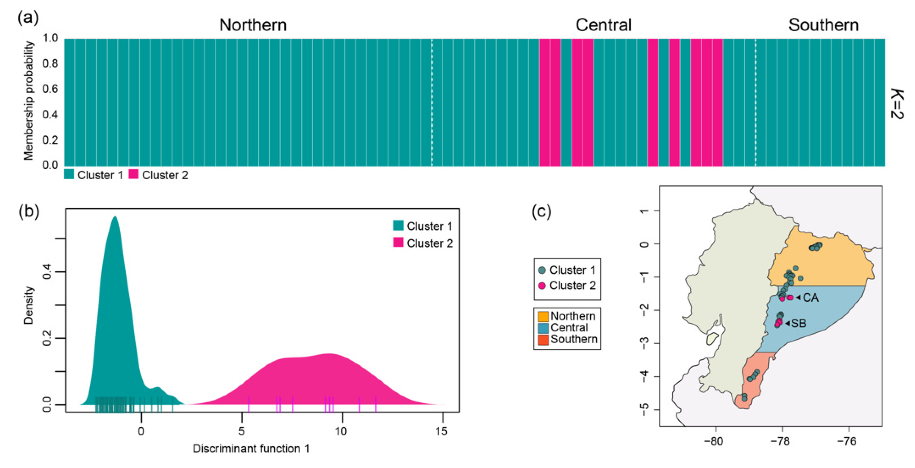
3.2. Population Structure

Pairwise FST values ranged from 0.017 to 0.029, revealing that the three Amazon regions exhibit a low degree of genetic differentiation [78]. The Northern and Southern regions were the least differentiated, while the Central and Southern regions were the most differentiated (Table S6). AMOVA analysis indicated that 97% of the total genetic variation was found within regions and 3% among regions (p-value = 0.0026) (Table 3).
DAPC results suggest the existence of two genetic clusters (Figure 2a), as measured by the AIC and KIC statistics (Figure S4). With this analysis, 67 individuals were classified within Cluster 1 (teal) and nine within Cluster 2 (pink). As seen in Figure 2b, with the discriminant function 1 of the DAPC, these two genetic clusters can be clearly differentiated. Geographically speaking, Cluster 1 comprised individuals from the three Amazon regions, while Cluster 2 included individuals from the Central region exclusively, located at specific collections sites known as “Canelos” and “Sevilla don Bosco” (Figure 2c).
The degree of genetic structure was further explored with a PCoA based on Bruvo’s distances, in which the first two axes explained 44% of the total variance. Statistically significant differences between the individuals’ clustering according to their region of origin can be seen in Figure 3a (p-value = 0.0011). Pairwise comparisons revealed that individuals from the Northern and Southern regions clustered together, showing no differences (p-value = 0.4020). In the case of the Central region, individuals distributed indistinctly in the PCoA plot. However, within this distribution, there were specific samples that separated from the rest through the variance explained by the first coordinate (PC1). For this reason, pairwise comparisons recognized the Central region as a statistically different group compared to the Northern (p-value = 0.0010) and Southern regions (p-value = 0.0210). Figure 3b illustrates that individuals form two separate groups representing the two genetic clusters previously found with the DAPC (p-value = 0.0001).

3.3. Isolation-by-Distance (IBD) and Isolation-by-Environment (IBE)

Geographic distances were not correlated to genetic distances (Mantel test p-value = 0.6623, r = −0.0278). Therefore, an IBD model does not seem to explain the observed population structure. However, environmental distances were significantly correlated to genetic distances (Mantel test p-value = 0.0059, r = 0.0945), suggesting that an IBE model could explain the genetic structure we found. Environmental variables’ influence as predictors of genetic distances was evaluated with a dbRDA (Figure 4). The model was considered statistically significant (p-value = 0.0002; adjusted R2 = 0.129), and the first two constrained axes explained 15.97% of the variance. Temperature seasonality (SD × 100) (Bio 4) and isothermality ×100 (Bio 3) were identified as significant environmental variables determining the genetic differentiation among clusters (p-value = 0.0020 and p-value = 0.0010, respectively).
Additionally, the linear regression model for the log-transformed PC1 scores, using the environmental variables as predictors, suggested that there is a significant linear relationship between the PC1, the temperature seasonality (SD × 100) (Bio 4) (β = 0.01437, p-value = 0.0001) and the annual mean diurnal range (Bio 2) (β = 0.06665, p-value = 0.0433) (adjusted R2 = 0.169). Finally, a Wilcoxon rank-sum test revealed that the values of Bio 4 for both genetic clusters were significantly different (mean Cluster 1 = 41.63 °C, mean Cluster 2 = 49.81 °C; p-value = 1.8888 × 10⁻⁵), as well as for Bio 3 (mean Cluster 1 = 87.90%, mean Cluster 2 = 86.03%, p-value = 0.0008). The values of Bio 2 for both clusters were not significantly different (p-value = 0.0631).

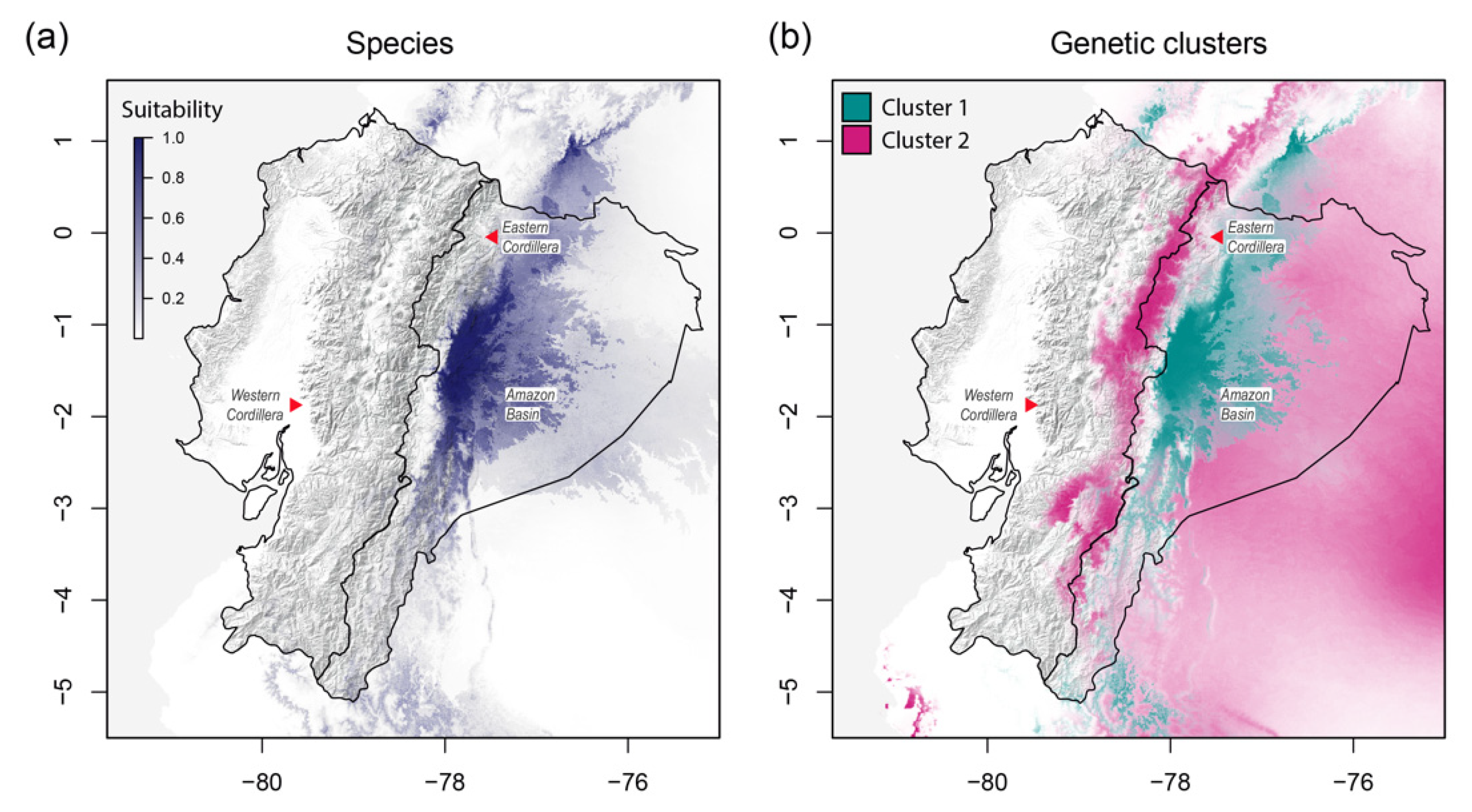
3.4. Niche Characterization Modeling

We modeled a total of three potential ecological niches for I. guayusa: one for the species and one for each of the other two genetic clusters identified in this study. We also obtained the mean AUC values for each model, which is a measurement of prediction accuracy. All AUC values were >0.9, therefore indicating that our models had an excellent prediction performance. According to the Schoener’s D statistic (Table 4), the predicted distribution range for Cluster 1 was the most similar with respect to that predicted for the species (D = 0.875). By contrast, the Cluster 2 distribution range was the most distinct (D = 0.426). Specifically, the suitable habitat for the species (Figure 5a) and Cluster 1 (Figure 5b in teal) was found mainly in the Ecuadorian Central Amazon, towards the Andean-Amazonian piedmont. For Cluster 2 the suitable habitat principally comprised the eastern slopes of the Andean cordillera and the eastern Amazon basin (Figure 5b in pink).
For each generated model, the bioclimatic variable importance was calculated in terms of its percentage contribution to the model’s fitness (Table 5). In this way, it was determined that the potential distribution range of the species and the Cluster 1 samples was mainly explained by the mean temperature of the wettest quarter (Bio 8) and the precipitation of the driest quarter (Bio 17) (Table 5). By contrast, Cluster 2 samples’ distribution range was mainly explained by the mean temperature of the wettest quarter (Bio 8) and the precipitation seasonality CV (Bio 15) (Table 5).

4. Discussion

4.1. A Moderately Low Genetic Diversity for Ilex guayusa in the Ecuadorian Amazon

In this study, we found that I. guayusa presents a moderately low genetic diversity (He = 0.396) in the Ecuadorian Amazon region. In a previous report, we assessed the preliminary genetic diversity of guayusa from the Ecuadorian Amazon using ISSRs markers and found that it was considerably lower than the one found with SSR markers (He = 0.19) [25]. Direct comparisons are not possible since the molecular markers used were different; however, the higher levels of genetic diversity found could be attributed to the high discriminating power of SSRs [79,80,81]. Additionally, SSRs markers have shown higher resolution to assess genetic diversity in clonal species when compared to ISSRs markers [82,83,84,85]. The present study also covered a greater sampling area, which could have contributed to the better genetic diversity characterization of the guayusa in the Ecuadorian Amazon.
SSRs markers have been previously used in Uruguay and Brazil to evaluate the genetic diversity in yerba mate (I. paraguariensis), a species closely related to guayusa. Obtained values of He ranged from 0.5 to 0.6 for Uruguay and Brazil, respectively, which were higher than the values of He found in our study [14,15]. This difference in genetic diversity could be explained by the fact that yerba mate is mainly propagated through sexual reproduction, which could increase genetic diversity [2]. In addition, I. paraguariensis is an allogamous species, which employs cross-fertilization as a reproductive strategy to promote intense gene flow between populations and, in this way, generate high levels of genetic diversity [86,87].
For clonal plants, the conservation of their genetic diversity could be promoted by a phenomenon called the “Meselson effect” [88,89]. Balloux et al. (2003) [88] suggested that the absence of sexual reproduction may lead to the accumulation of mutations over time, promoting genetic divergence between alleles within loci. This generates an excess of heterozygotes and negative FIS values, which are commonly reported within clonally reproducing species [90]. This could be the case of guayusa, where we found an overall negative FIS value (−0.185) and high Ho, similar to other clonally propagated plants [91,92,93].
The way in which guayusa has been cultivated and consumed could also be implicated in explaining the genetic diversity found. The earliest report of human utilization of this species can be traced back to 500 A.D.; however, its selection and domestication process began only in the late 1600s, when its extensive consumption was known to have been already established [10]. During this elapsed time, guayusa was being intermittently traded among indigenous communities [3], and until the present day has only been cultivated under a smallholder production model, which has shown to strengthen biodiversity conservation [94]. In commercially important crops, up to 10,000 years are needed to achieve full domestication [95], which could explain why guayusa is not yet considered a completely domesticated plant [3]. It is known that extended cultivation and selection periods are among the most critical factors causing genetic diversity erosion [95], which certainly is not the case for guayusa.
Concerning the genetic diversity found in each of the three regions of our study, we noted that the Central region harbored the greatest genetic diversity. Previous studies reported that the distribution of genetic diversity within the range of a species is often not uniform [93,96]. The “Abundant-Center Hypothesis” states that central populations tend to develop greater levels of genetic diversity. This phenomenon occurs fairly frequently [97,98,99] and needs to be further explored in guayusa.

4.2. High Clonal Diversity for Ilex guayusa in the Ecuadorian Amazon

In this study, we found high clonal diversity for I. guayusa (Simpson’s diversity index, D = 0.986–0.998; Shannon–Wiener index, ShW = 1.893–2.670), as was previously reported for another member of the Ilex genus (I. integra) [18]. Genotypic diversity assessment is important in clonal species because clonality can reduce the number of unique MLGs present in a population [100,101,102,103,104]. Regarding clonal diversity distribution, we found that individuals sharing identical MLGs were not necessarily close in proximity. It is known that certain means of vegetative propagation such as stolons, runners, and bulbils can result in this type of MLG distribution pattern, in which clones are located farther apart from the parental plant [105]. To the best of our knowledge, guayusa reproduction is mainly performed by human planting of stem cuttings [3]. Thus, the present distribution of the identified MLGs is most likely explained by secondary factors such as human activity [26].
Mechanisms for preserving clonal diversity in plants with poor or absent sexual reproduction could encompass multiple strategies. One of them is maintaining a clonal reproduction habit, since continuous propagation could lead to the long-term persistence of established MLGs in a population [27,92]. In that way, the only means by which an MLG could be lost is by the death of all the individuals harboring this MLG [27]. This is relatively uncommon for long-lived species such as guayusa, whose trees can live for hundreds of years according to various ethnobotanical observations [4]. As the species is long-lived, there is also a probability that the MLGs in existence today are clones from the original MLGs established among the founder populations [27,92]. In this way, we could still be analyzing some part of the species’ initial clonal diversity, when sexual reproduction was not as limited as today [106]. All these factors could account for the high clonal diversity observed in guayusa.
Additionally, truly clonal individuals are considered “immune” to the diversifying effect of recombination occurring during sexual reproduction [107]. This preserves MLGs over time because whenever the gene pool is reshuffled during reproduction, the alleles can be lost by chance, especially in small populations [27]. Nonetheless, we cannot rule out the probability that occasional sexual reproduction events could occur, as has been suggested for other species [89,104]. Regardless of the idea that guayusa does not bloom [4], studies suggest that even in fully domesticated plants with lost sexual fertility, sexual reproduction still occurs at a negligible rate in semi-domesticated varieties [28]. Most forest tree species, like guayusa, are at an early stage of domestication [95], and therefore, it is probable that they still conserve effective means of sexual reproduction.

4.3. Influence of the Environment and Human Activities as Modulators of Ilex guayusa Population Structure

The DAPC suggested the existence of two genetic clusters. The PCoAs on Bruvo’s distances further confirmed that individuals clustered in two different groups. Together with the low values of the F-statistics and the large intrapopulation genetic variability calculated by the AMOVA, these results suggest that I. guayusa has a shallow and subtle population structure across the Ecuadorian Amazon. Previous studies have identified geographic distance as a key factor affecting a species’ genetic structure [62,108]. However, we did not find evidence that an increase in the geographic distance was correlated with an increase in genetic differentiation. For example, Cluster 1 grouped distant individuals, such as those belonging to the Northern and Southern regions, independently of the geographic distance existing between them. Similarly, Cluster 2 grouped only individuals belonging to Canelos and Sevilla Don Bosco (two specific localities at the Central Amazon), while other individuals in the proximity were completely excluded. For this reason, we propose that a model of IBD does not explain the genetic structure that we found for I. guayusa, and suggest that the model of IBE could explain it. We corroborated that the environmental distances were correlated to the genetic distances with a Mantel test, indicating that climatic and habitat conditions have played a role in determining the population structure of this species.
IBD appears to be more frequently reported in plants than IBE [98]. However, this may be due to the recent recognition of the environment’s role in shaping spatial patterns of gene flow and genetic variation [109,110,111]. Nowadays, IBE is known as a widespread but complex phenomenon in nature [98,112], driving genotypic and phenotypic divergence in several taxa, including tree species like Fraxinus angustifolia Vahl [113], Alnus incana (L.) Moench [114], Populus nigra L. [115], and Sequoiadendron giganteum (Lindl.) J.Buchholz [116]. It should be considered that IBE does not operate in isolation and can interact with geography, colonization, selection, gene flow, and genetic drift as well [117,118]. For this reason, studying observed patterns of spatial genetic differentiation caused by IBE is coupled with several challenges, such as disentangling the effect of correlated variables and determining the processes that have generated and maintained the observed IBE patterns [111].
To deepen into the processes driving genetic differentiation, a linear regression model and a dbRDA, which is a method used to assess the influence of environmental variables on population structure, led us to suggest that among the studied bioclimatic variables, the one that best explained the genetic differentiation of Cluster 2 in guayusa was the temperature seasonality SD × 100 (Bio 4). This bioclimatic variable is defined as the amount of temperature variation over a given year. Previous studies have determined that Bio 4 can demographically isolate populations by environmental climate heterogeneity, which will promote genetic divergence within the species [119,120]. Temperature seasonality has also been demonstrated to affect the caffeine concentration in species like tea [121] and yerba mate [122]. Caffeine is a principal chemical constituent produced among many species of the Ilex genus [123], and in the case of I. guayusa, variable concentrations of caffeine can result in a broad range of desired and undesired physiological effects when consumed [1]. In 1991, Lewis et al. highlighted the importance of experiential learning as a factor for the human selection of I. guayusa individuals [1]. They observed that cultivars of guayusa known to produce unsettling symptoms after consumption were rarely propagated among indigenous communities. They further suggested that plant populations with specific chemical profiles can harbor genetic differences as well, and therefore, the selection of I. guayusa cultivars based on their chemical profile may have potentially affected the population structure seen nowadays [1].
We predicted the potential distribution range for I. guayusa at the species level and for each of the genetic clusters identified. Our results highlighted the presence of niche dissimilarities for each of the genetic clusters found. Previous studies have reported this pattern, in which predicted niches could vary between genetic groups within a species [120,124] since they are usually more environmentally compact and tuned to specific climatic conditions [120]. We observed that the potential distribution range of I. guayusa at the species level and for Cluster 1 was mainly explained by the mean temperature of the wettest quarter (Bio 8) and the precipitation of the driest quarter (Bio 17). On the other hand, genetic Cluster 2 exhibited a different combination of environmental variables that explained its potential distribution range, mainly precipitation seasonality CV (Bio 15). In addition, we predicted that Cluster 2 could occupy landscapes towards the range limits of the species’ distribution. At these marginal or borderline habitats, populations can develop unique genetic variation due to local adaptations to the occurring environmental conditions [93]. This may promote the genetic divergence of peripheral populations, causing IBE patterns of genetic differentiation as observed in this study for guayusa.
Even though more studies are needed, the possibility that certain guayusa genotypes might have adaptations to specific climatic conditions is of great interest in the context of climate change and species conservation. This study emphasizes the usefulness of using SSRs to identify genotypes whose conservation should be prioritized. Incorporating genetic information into the modeling of a species’ distribution range is important because it can help identify specific variables and environmental drivers that could account for the observed genetic structure [120]. Moreover, including genetic information can improve modeling accuracy when predicting a species’ potential distribution under climate change scenarios, giving important cues for its conservation in the future [124].
We have discussed how environmental factors may have affected the genetic structure of I. guayusa. However, genetic diversity is a complex interplay between several evolutionary phenomena [95], in which we cannot dismiss human activity as an additional factor that may have influenced I. guayusa genetic structure. Historical records indicate that due to guayusa trading, the commercial relationships between the Andes and the Amazon intensified [125]. In Ecuador, the Bobonaza and the Pastaza rivers were considered key fluvial routes for transportation and commercialization between the Central Amazon and the Central Andes [126], which could have strategically connected human settlements located alongside these rivers. Examples of this in the Ecuadorian Amazon are Canelos and its adjacent valleys, which hold great importance in the guayusa cultivation history [7,10] since they are suspected to be the real centers of guayusa cultivation [4]. Around 1850, the use and cultivation of guayusa were thought to be confined to these locations, and in the same decade, the existence of a group of guayusa trees from the pre-Columbian period on an ancient site called Antombós, located in the Central Andes at the gorge of the Pastaza river, was reported [4,5,7,127]. As guayusa was increasingly traded between regions, this could have led to the migration of individuals from both guayusa populations, shaping the genetic structure that the species has today. We found that the samples from Canelos grouped within Cluster 2, which might serve as evidence of guayusa’s trading and cultivation history. Further analyses that include samples from the eastern Central Andes could shed light of the composition of Cluster 2.
With these preliminary results, a more thorough sampling of individuals at multiple locations should be performed to better understand the genetic diversity and demographic history of guayusa. Moreover, we highlight the environmental plasticity found within this clonal species as a key feature for its success [105,128] as it could help overcome genetic diversity erosion and environmental changes [28]. The identification of populations adapted to diverse environments and different ranges of distribution is of great importance for the conservation of I. guayusa. Usually, these populations harbor unique genetic pools that could make them more resilient to environmental changes, which in the near future could help maintain the species’ ability to evolve and adapt [62,93].

5. Conclusions

This study offers a first glance at the genetic diversity of I. guayusa in the Ecuadorian Amazon region. The species showed a moderately low genetic diversity and high clonal diversity. Two genetic clusters were identified among the 71 individuals with unique MLGs. We suggest that the population structure found might be explained by a model of IBE. Temperature seasonality (SD × 100) (Bio 4) and isothermality ×100 (Bio 3) were found to have an important influence on how the guayusa genetic clusters are distributed. Nonetheless, further studies are needed to fully understand its genetic diversity and population structure. It is relevant to establish conservation strategies and sustainable use of guayusa since it is considered an important agroforestry resource. Different approaches should be considered, such as studying the possible occurrence of sexual reproduction and maintaining the chacra agroforestry model based on a smallholder-based production system. Conserving its genetic and clonal diversity is key to establishing successful long-term breeding programs, which will promote the economic growth of local communities and reinforce the value of ancestral knowledge.

Supplementary Materials

The following are available online at https://www.mdpi.com/article/10.3390/d13050182/s1, Figure S1: Frequency distribution of the pairwise Bruvo’s genetic distances (transformed between 0 and 100) for 88 Ilex guayusa individuals genotyped with 17 SSR markers. Following the assumption that the histograms of the pairwise comparisons are often multimodal, the valley between the first and second peak was considered as a good candidate to use as a threshold. At a threshold = 2, the inferred number of MLGs was 71. Figure S2: Genotype accumulation curve describing the genotypic resolution of the 17 SSR markers used in this study. All the employed markers were sufficient to identify and discriminate between the 71 MLGs. Figure S3: Histogram of the frequency of the F (inbreeding coefficient) values observed within the 76 Ilex guayusa individuals selected after clone correction. The data follow a right-skewed non-normal distribution. Figure S4: Goodness-of-fit statistics obtained for the determination of the optimal number of genetic clusters (K) using a maximum-likelihood approach. (a) Akaike information criterion (AIC) values plotted against a determined number of K; (b) Kullback Information Criterion (KIC) values plotted against a determined number of K. Table S1: Associated information to the Ilex guayusa samples collected for this study in the Ecuadorian Amazon. Table S2: Information of SSR-specific primers designed for Ilex guayusa. Table S3: Inferred MLG for each sample as calculated by GenoDive, using a genetic distance threshold of 2. Table S4: Results of the Hardy–Weinberg Equilibrium (HWE) test for each locus, after a Bonferroni correction. Table S5: Null allele frequencies estimation for each analyzed region and SSR locus. Table S6: Pairwise FST values calculated for the three Ecuadorian Amazon regions.

Author Contributions

Conceptualization: M.d.L.T.; methodology, M.P.E.-G., J.K.R., N.E.d.l.M.-S. and M.d.L.T.; software, M.P.E.-G., P.B.-S. and J.K.R.; validation, M.P.E.-G., J.K.R., P.B.-S., N.E.d.l.M.-S. and J.J.G.; formal analysis, M.P.E.-G., P.B.-S., N.E.d.l.M.-S. and J.J.G.; investigation, M.P.E.-G., P.B.-S. and N.E.d.l.M.-S.; resources, M.d.L.T.; data curation, M.P.E.-G., J.K.R., P.B.-S., N.E.d.l.M.-S. and J.J.G.; writing—original draft preparation, M.P.E.-G., P.B.-S., N.E.d.l.M.-S. and J.J.G.; writing—review and editing, M.P.E.-G., P.B.-S., N.E.d.l.M.-S., J.J.G. and M.d.L.T.; visualization, M.P.E.-G., P.B.-S., N.E.d.l.M.-S. and J.J.G.; supervision, M.d.L.T.; project administration, M.d.L.T.; funding acquisition, M.d.L.T. All authors have read and agreed to the published version of the manuscript.

Funding

This research was funded by Universidad San Francisco de Quito (USFQ) Grant Program, HUBi No. 7693 and 17149.

Institutional Review Board Statement

Not applicable.

Informed Consent Statement

Not applicable.

Data Availability Statement

Not applicable.

Acknowledgments

We would like to thank Daniela Rojas for the preliminary assessment of I. guayusa diversity and acknowledge RUNA Foundation for their participation at the beginning of the project in the collection of I. guayusa samples. The authors would like to thank the technical assistance and valuable insights offered by the members of the Plant Biotechnology Laboratory (COCIBA, USFQ). This study was carried out following Ecuadorian regulations (Contrato Marco de Acceso a los Recursos Genéticos MAE-DNB-CM-2016-0046).

Conflicts of Interest

The authors declare no conflict of interest. The funders had no role in the design of the study; in the collection, analyses, or interpretation of data; in the writing of the manuscript, or in the decision to publish the results.

References

  1. Lewis, W.H.; Kennelly, E.J.; Bass, G.N.; Wedner, H.J.; Elvin-Lewis, M.P.; Fast, D. Ritualistic use of the holly Ilex guayusa by Amazonian Jivaro Indians. J. Ethnopharmacol. 1991, 33, 25–30. [Google Scholar] [CrossRef]
  2. Sequeda-Castañeda, L.G.; Modesti Costa, G.; Celis, C.; Gamboa, F.; Gutiérrez, S.; Luengas, P. Ilex guayusa Loes (Aquifoliaceae): Amazon and Andean native plant. Pharmacol. OnLine 2016, 3, 193–202. [Google Scholar]
  3. Dueñas, J.F.; Jarrett, C.; Cummins, I.; Logan-Hines, E. Amazonian Guayusa (Ilex guayusa Loes.): A Historical and Ethnobotanical Overview. Econ. Bot. 2016, 70, 85–91. [Google Scholar] [CrossRef]
  4. Schultes, R.E. Ilex guayusa from 500 A.D. to the present. In Etnologiska Studier; Göteborgs Etnografiska Museum: Göteborg, Sweden, 1972; Volume 32, pp. 115–138. [Google Scholar]
  5. Wassen, H. A Medicine-man’s Implements and Plants in a Tiahuanacoid Tomb in Highland Bolivia. In Etnologiska Studier; Göteborgs Etnografiska Museum: Göteborg, Sweden, 1972; Volume 32, pp. 8–114. [Google Scholar]
  6. Kapp, R.W.; Mendes, O.; Roy, S.; McQuate, R.S.; Kraska, R. General and Genetic Toxicology of Guayusa Concentrate (Ilex guayusa). Int. J. Toxicol. 2016, 35, 222–242. [Google Scholar] [CrossRef] [Green Version]
  7. Schultes, R.E. Discovery of an ancient guayusa plantation in Colombia. Bot. Mus. Leafl. Harv. Univ. 1979, 27, 143–153. [Google Scholar] [CrossRef]
  8. García-Ruiz, A.; Baenas, N.; Benítez-González, A.M.; Stinco, C.M.; Meléndez-Martínez, A.J.; Moreno, D.A.; Ruales, J. Guayusa (Ilex guayusa L.) new tea: Phenolic and carotenoid composition and antioxidant capacity. J. Sci. Food Agric. 2017, 97, 3929–3936. [Google Scholar] [CrossRef]
  9. Radice, M.; Cossio, N.; Scalvenzi, L. Ilex guayusa: A systematic review of its Traditional Uses, Chemical Constituents, Biological Activities and Biotrade Opportunities. In MOL2NET: FROM MOLECULES TO NETWORKS, Proceedings of the MOL2NET 2016, International Conference on Multidisciplinary Sciences, Basel, Switzerland, 15 January–15 December 2016, 2nd ed.; MDPI: Basel, Switzerland, 2017; pp. 1–7. [Google Scholar]
  10. Patino, V.M. Guayusa, a neglected stimulant from the eastern Andean foothills. Econ. Bot. 1968, 22, 311–316. [Google Scholar] [CrossRef]
  11. Wise, G.; Santander, D.E. Assessing the History of Safe Use of Guayusa. J. Food Nutr. Res. 2018, 6, 471–475. [Google Scholar] [CrossRef]
  12. Shemluck, M. The Flowers of Ilex guayusa. Bot. Mus. Leafl. Harv. Univ. 1979, 27, 155–160. [Google Scholar]
  13. GBIF Backbone Taxonomy. Ilex guayusa Loes. in GBIF Secretariat. Available online: https://www.gbif.org/species/5534620 (accessed on 24 June 2020).
  14. Cascales, J.; Bracco, M.; Poggio, L.; Gottlieb, A.M. Genetic diversity of wild germplasm of “yerba mate” (Ilex paraguariensis St. Hil.) from Uruguay. Genetica 2014, 142, 563–573. [Google Scholar] [CrossRef]
  15. Pereira, M.F.; Ciampi, A.Y.; Inglis, P.W.; Souza, V.A.; Azevedo, V.C.R. Shotgun Sequencing for Microsatellite Identification in Ilex paraguariensis (Aquifoliaceae). Appl. Plant Sci. 2013, 1, 1–3. [Google Scholar] [CrossRef]
  16. Gauer, L.; Cavalli-Molina, S. Genetic variation in natural populations of maté (Ilex paraguariensis A. St.-Hil., Aquifoliaceae) using RAPD markers. Heredity 2000, 84, 647–656. [Google Scholar] [CrossRef]
  17. Chen, W.-W.; Xiao, Z.-Z.; Tong, X.; Liu, Y.-P.; Li, Y.-Y. Development and characterization of 25 microsatellite primers for Ilex chinensis (Aquifoliaceae). Appl. Plant Sci. 2015, 3, 1500057. [Google Scholar] [CrossRef] [PubMed]
  18. Torimaru, T.; Tomaru, N.; Nishimura, N.; Yamamoto, S. Clonal diversity and genetic differentiation in Ilex leucoclada M. patches in an old-growth beech forest. Mol. Ecol. 2003, 12, 809–818. [Google Scholar] [CrossRef]
  19. Rendell, S.; Ennos, R.A. Chloroplast DNA diversity of the dioecious European tree Ilex aquifolium L. (English holly). Mol. Ecol. 2003, 12, 2681–2688. [Google Scholar] [CrossRef]
  20. Zhang, J.H.; Gao, Y.Z.; Zhang, B.; Wang, Z.J. Genetic diversity of Ilex L. tree species. Acta Bot. Boreali Occident. Sin. 2011, 31, 504–510. [Google Scholar]
  21. Xi-Jun, Z.; Dong-Mei, Z.; Yu-Lan, L.; Jin-Le, S.; Jian-Xiang, L. Inter-simple sequence repeats (ISSR) marker analysis of flex plants species and its application. J. Henan Agric. Univ. 2009, 43, 196–200. [Google Scholar]
  22. Qian, Y.S.; Wang, H.Z.; Shi, N.N.; Zhao, Y.; Li, N.L.; Hu, Z. Studies of genetic diversity among 10 species of Ilex based on RAPD and AFLPs. J. Mol. Cell Biol. 2008, 41, 35–43. [Google Scholar]
  23. Heck, C.; de Mejia, E. Yerba Mate Tea (Ilex paraguariensis): A Comprehensive Review on Chemistry, Health Implications, and Technological Considerations. J. Food Sci. 2007, 72, R138–R151. [Google Scholar] [CrossRef]
  24. Kothiyal, S.K.; Sati, S.C.; Rawat, M.S.M.; Sati, M.D.; Semwal, D.K.; Semwal, R.B.; Sharma, A.; Rawat, B.; Kumar, A. Chemical Constituents and Biological Significance of the Genus Ilex (Aquifoliaceae). Nat. Prod. J. 2012, 2, 212–224. [Google Scholar] [CrossRef]
  25. Salvador, A.T.; Mosquera, J.; Jaramillo, V.; Arahana, V.; Torres, M.D.L. Preliminary assessment of the degree of genetic diversity of Ecuadorean Ilex guayusa using inter simple sequence repeat (ISSR) markers. ACI Av. Cienc. Ing. 2017, 9. [Google Scholar] [CrossRef] [Green Version]
  26. Brzosko, E.; Wróblewska, A.; Ratkiewicz, M. Spatial genetic structure and clonal diversity of island populations of lady’s slipper (Cypripedium calceolus) from the Biebrza National Park (northeast Poland). Mol. Ecol. 2002, 11, 2499–2509. [Google Scholar] [CrossRef]
  27. Pleasants, J.M.; Wendel, J.F. Genetic Diversity in a Clonal Narrow Endemic, Erythronium propullans, and in Its Widespread Progenitor, Erythronium albidum. Am. J. Bot. 1989, 76, 1136–1151. [Google Scholar] [CrossRef]
  28. McKey, D.; Elias, M.; Pujol, B.; Duputié, A. The evolutionary ecology of clonally propagated domesticated plants. N. Phytol. 2010, 186, 318–332. [Google Scholar] [CrossRef]
  29. Environmental Systems Research Institute. ArcGIS Desktop: Release 10. Available online: https://desktop.arcgis.com/es/ (accessed on 18 June 2020).
  30. Križman, M.; Jakše, J.; Baričevič, D.; Javornik, B.; Prošek, M. Robust CTAB-activated charcoal protocol for plant DNA extraction. Acta Agric. Slov. 2006, 87, 427–433. [Google Scholar]
  31. Rezadoost, M.H.; Kordrostami, M.; Kumleh, H.H. An efficient protocol for isolation of inhibitor-free nucleic acids even from recalcitrant plants. 3 Biotech 2016, 6, 1–7. [Google Scholar] [CrossRef] [PubMed] [Green Version]
  32. Griffiths, S.M.; Fox, G.; Briggs, P.J.; Donaldson, I.J.; Hood, S.; Richardson, P.; Leaver, G.W.; Truelove, N.K.; Preziosi, R.F. A Galaxy-based bioinformatics pipeline for optimised, streamlined microsatellite development from Illumina next-generation sequencing data. Conserv. Genet. Resour. 2016, 8, 481–486. [Google Scholar] [CrossRef] [PubMed] [Green Version]
  33. Andrews, S. FastQC: A Quality Control Tool for High Throughput Sequence Data 2010; Babraham Institute: Cambridge, UK, 2014; Available online: https://www.bioinformatics.babraham.ac.uk/projects/fastqc/ (accessed on 10 January 2018).
  34. Bolger, A.M.; Lohse, M.; Usadel, B. Trimmomatic: A flexible trimmer for Illumina sequence data. Bioinformatics 2014, 30, 2114–2120. [Google Scholar] [CrossRef] [PubMed] [Green Version]
  35. Castoe, T.A.; Poole, A.W.; de Koning, A.P.J.; Jones, K.L.; Tomback, D.F.; Oyler-McCance, S.J.; Fike, J.A.; Lance, S.L.; Streicher, J.W.; Smith, E.N.; et al. Rapid Microsatellite Identification from Illumina Paired-End Genomic Sequencing in Two Birds and a Snake. PLoS ONE 2012, 7, e30953. [Google Scholar] [CrossRef] [Green Version]
  36. Koressaar, T.; Remm, M. Enhancements and modifications of primer design program Primer3. Bioinformatics 2007, 23, 1289–1291. [Google Scholar] [CrossRef] [Green Version]
  37. Untergasser, A.; Cutcutache, I.; Koressaar, T.; Ye, J.; Faircloth, B.C.; Remm, M.; Rozen, S.G. Primer3—New capabilities and interfaces. Nucleic Acids Res. 2012, 40, e115. [Google Scholar] [CrossRef] [Green Version]
  38. Blacket, M.J.; Robin, C.; Good, R.T.; Lee, S.F.; Miller, A.D. Universal primers for fluorescent labelling of PCR fragments—An efficient and cost-effective approach to genotyping by fluorescence. Mol. Ecol. Resour. 2012, 12, 456–463. [Google Scholar] [CrossRef]
  39. Hulce, D.; Li, X.; Snyder-Leiby, T.; Liu, C.J. GeneMarker® Genotyping Software: Tools to Increase the Statistical Power of DNA Fragment Analysis. J. Biomol. Tech. 2011, 22, S35–S36. [Google Scholar]
  40. Meirmans, P.G.; van Tienderen, P.H. Genotype and genodive: Two programs for the analysis of genetic diversity of asexual organisms. Mol. Ecol. Notes 2004, 4, 792–794. [Google Scholar] [CrossRef]
  41. Bruvo, R.; Michiels, N.K.; D’Souza, T.G.; Schulenburg, H. A simple method for the calculation of microsatellite genotype distances irrespective of ploidy level. Mol. Ecol. 2004, 13, 2101–2106. [Google Scholar] [CrossRef]
  42. Kamvar, Z.N.; Tabima, J.F.; Grünwald, N.J. Poppr: An R package for genetic analysis of populations with clonal, partially clonal, and/or sexual reproduction. PeerJ 2014, 2, e281. [Google Scholar] [CrossRef] [Green Version]
  43. R Core Team. R: A Language and Environment for Statistical Computing; R Foundation for Statistical Computing: Vienna, Austria, 2018; Available online: https://www.R-project.org/ (accessed on 29 February 2020).
  44. Pluess, A.R.; Stöcklin, J. Population genetic diversity of the clonal plant Geum reptans (Rosaceae) in the Swiss Alps. Am. J. Bot. 2004, 91, 2013–2021. [Google Scholar] [CrossRef]
  45. Parks, J.C.; Werth, C.R. A Study of Spatial Features of Clones in a Population of Bracken Fern, Pteridium aquilinum (Dennstaedtiaceae). Am. J. Bot. 1993, 80, 537. [Google Scholar] [CrossRef]
  46. Goudet, J. hierfstat, a package for R to compute and test hierarchical F-statistics. Mol. Ecol. Notes 2005, 5, 184–186. [Google Scholar] [CrossRef] [Green Version]
  47. Jombart, T.; Bateman, A. adegenet: A R package for the multivariate analysis of genetic markers. Bioinformatics 2008, 24, 1403–1405. [Google Scholar] [CrossRef] [Green Version]
  48. Keenan, K.; McGinnity, P.; Cross, T.F.; Crozier, W.W.; Prodöhl, P.A. diveRsity: An R package for the estimation and exploration of population genetics parameters and their associated errors. Methods Ecol. Evol. 2013, 4, 782–788. [Google Scholar] [CrossRef] [Green Version]
  49. Clark, L.V.; Jasieniuk, M. polysat: An R package for polyploid microsatellite analysis. Mol. Ecol. Resour. 2011, 11, 562–566. [Google Scholar] [CrossRef]
  50. Chapuis, M.-P.; Estoup, A. Microsatellite Null Alleles and Estimation of Population Differentiation. Mol. Biol. Evol. 2006, 24, 621–631. [Google Scholar] [CrossRef] [PubMed] [Green Version]
  51. Paradis, E. pegas: An R package for population genetics with an integrated-modular approach. Bioinformatics 2010, 26, 419–420. [Google Scholar] [CrossRef] [PubMed] [Green Version]
  52. Peakall, R.; Smouse, P.E. GenAlEx 6.5: Genetic analysis in Excel. Population genetic software for teaching and research—An update. Bioinformatics 2012, 28, 2537–2539. [Google Scholar] [CrossRef] [PubMed] [Green Version]
  53. Jombart, T.; Devillard, S.; Balloux, F. Discriminant analysis of principal components: A new method for the analysis of genetically structured populations. BMC Genet. 2010, 11, 94. [Google Scholar] [CrossRef] [Green Version]
  54. Grünwald, N.J.; Everhart, S.E.; Knaus, B.J.; Kamvar, Z.N. Best Practices for Population Genetic Analyses. Phytopathology 2017, 107, 1000–1010. [Google Scholar] [CrossRef] [Green Version]
  55. Beugin, M.; Gayet, T.; Pontier, D.; Devillard, S.; Jombart, T. A fast likelihood solution to the genetic clustering problem. Methods Ecol. Evol. 2018, 9, 1006–1016. [Google Scholar] [CrossRef] [Green Version]
  56. Paradis, E.; Schliep, K. ape 5.0: An environment for modern phylogenetics and evolutionary analyses in R. Bioinformatics 2018, 35, 526–528. [Google Scholar] [CrossRef]
  57. Oksanen, J.; Blanchet, G.; Friendly, M.; Kindt, R.; Legendre, P.; McGlinn, D.; Minchin, P.; O’Hara, R.; Simpson, G.; Solymos, P.; et al. vegan: Community Ecology Package; Version 2.5–6. Available online: https://CRAN.R-project.org/package=vegan (accessed on 19 September 2020).
  58. Kindt, R.; Coe, R. A Manual and Software for Common Statistical Methods for Ecological and Biodiversity Studies. In Tree Diversity Analysis, 1st ed.; World Agroforestry Centre (ICRAF): Nairobi, Kenya, 2005; ISBN 92-9059-179-X. [Google Scholar]
  59. Fick, S.E.; Hijmans, R.J. WorldClim 2: New 1-km spatial resolution climate surfaces for global land areas. Int. J. Climatol. 2017, 37, 4302–4315. [Google Scholar] [CrossRef]
  60. Hijmans, R. raster: Geographic Data Analysis and Modeling; Version 3.1–5. Available online: https://CRAN.R-project.org/package=raster (accessed on 19 September 2020).
  61. Kuhn, M. Building Predictive Models in R Using the caret Package. J. Stat. Softw. 2008, 28, 1–26. [Google Scholar] [CrossRef] [Green Version]
  62. Jiang, S.; Luo, M.-X.; Gao, R.-H.; Zhang, W.; Yang, Y.-Z.; Li, Y.-J.; Liao, P.-C. Isolation-by-environment as a driver of genetic differentiation among populations of the only broad-leaved evergreen shrub Ammopiptanthus mongolicus in Asian temperate deserts. Sci. Rep. 2019, 9, 12008–12014. [Google Scholar] [CrossRef]
  63. Hijmans, R. geosphere: Spherical Trigonometry; Version 1.5–10. Available online: https://CRAN.R-project.org/package=geosphere (accessed on 19 September 2020).
  64. Venables, W.; Ripley, B. Modern Applied Statistics with S, 4th ed.; Springer: New York, NY, USA, 2002; ISBN 978-0-387-21706-2. [Google Scholar]
  65. Phillips, S.; Dudik, M.; Schapire, R. Maxent Software for Modeling Species Niches and Distributions; Version 3.4.1; American Museum of Natural History: New York, NY, USA, 2021; Available online: http://biodiversityinformatics.amnh.org/open_source/maxent/ (accessed on 25 June 2020).
  66. University of California, Davis. DAV—UC Davis Herbarium; Center for Plant Diversity: Davis, CA, USA, 2020; Available online: https://www.gbif.org/dataset/c267909d-184f-4138-9e67-a074d478d52b (accessed on 24 June 2020).
  67. Ramirez, J.; Tulig, M.; Watson, K.; Thiers, B. The New York Botanical Garden Herbarium (NY); Version 1.22; The New York Botanical Garden: New York, NY, USA, 2020; Available online: https://www.gbif.org/dataset/d415c253-4d61-4459-9d25-4015b9084fb0 (accessed on 24 June 2020).
  68. Institute of Botany, University of Hohenheim. Visual Plants (144.41.33.158)—Private Collection of Rainer Bussmann. Available online: https://www.gbif.org/dataset/85cf474e-f762-11e1-a439-00145eb45e9a (accessed on 24 June 2020).
  69. Crop Wild Relatives Occurrence data consortia. A Global Database for the Distributions of Crop Wild Relatives; Version 1.12; Centro Internacional de Agricultura Tropical—CIAT: Cali, Colombia, 2018; Available online: https://www.gbif.org/dataset/07044577-bd82-4089-9f3a-f4a9d2170b2e (accessed on 24 June 2020).
  70. Ueda, K. iNaturalist Research-grade Observations; iNaturalist.org. Available online: https://www.gbif.org/dataset/50c9509d-22c7-4a22-a47d-8c48425ef4a7 (accessed on 24 June 2020).
  71. Orrell, T. NMNH Extant Specimen Records; Version 1.32; National Museum of Natural History, Smithsonian Institution: Washington, DC, USA, 2020; Available online: https://www.gbif.org/dataset/821cc27a-e3bb-4bc5-ac34-89ada245069d (accessed on 24 June 2020).
  72. Herbarium of the University of Aarhus. The AAU Herbarium Database. Available online: https://www.gbif.org/dataset/833db434-f762-11e1-a439-00145eb45e9a (accessed on 24 June 2020).
  73. Grant, S.; Niezgoda, C. Field Museum of Natural History (Botany) Seed Plant Collection; Version 11.12; Field Museum: Chicago, IL, USA, 2020; Available online: https://www.gbif.org/dataset/90c853e6-56bd-480b-8e8f-6285c3f8d42b (accessed on 24 June 2020).
  74. Magill, B.; Solomon, J.; Stimmel, H. Tropicos Specimen Data; Missouri Botanical Garden: St. Louis, MO, USA, 2020; Available online: https://www.gbif.org/dataset/7bd65a7a-f762-11e1-a439-00145eb45e9a (accessed on 24 June 2020).
  75. Aiello-Lammens, M.E.; Boria, R.A.; Radosavljevic, A.; Vilela, B.; Anderson, R.P. spThin: An R package for spatial thinning of species occurrence records for use in ecological niche models. Ecography 2015, 38, 541–545. [Google Scholar] [CrossRef]
  76. Jayasinghe, S.L.; Kumar, L. Modeling the climate suitability of tea (Camellia sinensis (L.) O. Kuntze) in Sri Lanka in response to current and future climate change scenarios. Agric. For. Meteorol. 2019, 272–273, 102–117. [Google Scholar] [CrossRef]
  77. Warren, D.L.; Glor, R.E.; Turelli, M. ENMTools: A toolbox for comparative studies of environmental niche models. Ecography 2010, 33, 607–611. [Google Scholar] [CrossRef]
  78. Balloux, F.; Lugon-Moulin, N. The estimation of population differentiation with microsatellite markers. Mol. Ecol. 2002, 11, 155–165. [Google Scholar] [CrossRef] [PubMed] [Green Version]
  79. Vieira, M.L.C.; Santini, L.; Diniz, A.L.; Munhoz, C.D.F. Microsatellite markers: What they mean and why they are so useful. Genet. Mol. Biol. 2016, 39, 312–328. [Google Scholar] [CrossRef]
  80. Powell, W.; Machray, G.C.; Provan, J. Polymorphism revealed by simple sequence repeats. Trends Plant Sci. 1996, 1, 215–222. [Google Scholar] [CrossRef]
  81. Kalia, R.K.; Rai, M.K.; Kalia, S.; Singh, R.; Dhawan, A.K. Microsatellite markers: An overview of the recent progress in plants. Euphytica 2010, 177, 309–334. [Google Scholar] [CrossRef]
  82. Forneck, A. Plant Breeding: Clonality—A Concept for Stability and Variability During Vegetative Propagation. In Progress in Botany; Esser, K., Lüttge, U., Beyschlag, W., Murata, J., Eds.; Springer: Berlin/Heidelberg, Germany, 2005; Volume 66, pp. 164–183. [Google Scholar]
  83. Arnaud-Haond, S.; Alberto, F.; Teixeira, S.; Procaccini, G.; Serrão, E.A.; Duarte, C.M. Assessing Genetic Diversity in Clonal Organisms: Low Diversity or Low Resolution? Combining Power and Cost Efficiency in Selecting Markers. J. Hered. 2005, 96, 434–440. [Google Scholar] [CrossRef] [Green Version]
  84. Ismail, N.A.; Rafii, M.Y.; Mahmud, T.M.M.; Hanafi, M.M.; Miah, G. Genetic Diversity of Torch Ginger (Etlingera elatior) Germplasm Revealed by ISSR and SSR Markers. BioMed Res. Int. 2019, 2019, 1–14. [Google Scholar] [CrossRef] [Green Version]
  85. Serra, I.; Procaccini, G.; Intrieri, M.; Migliaccio, M.; Mazzuca, S.; Innocenti, A. Comparison of ISSR and SSR markers for analysis of genetic diversity in the seagrass Posidonia oceanica. Mar. Ecol. Prog. Ser. 2007, 338, 71–79. [Google Scholar] [CrossRef]
  86. Júnior, E.L.C.; Donaduzzi, C.M.; Ferrarese-Filho, O.; Friedrich, J.C.; Gonela, A.; Sturion, J.A. Quantitative genetic analysis of methylxanthines and phenolic compounds in mate progenies. Pesqui. Agropecuária Bras. 2010, 45, 171–177. [Google Scholar] [CrossRef]
  87. Tarragó, J.; Sansberro, P.; Filip, R.; López, P.; González, A.; Luna, C.; Mroginski, L. Effect of leaf retention and flavonoids on rooting of Ilex paraguariensis cuttings. Sci. Hortic. 2005, 103, 479–488. [Google Scholar] [CrossRef]
  88. Balloux, F.; Lehmann, L.; de Meeûs, T. The population genetics of clonal and partially clonal diploids. Genetics 2003, 164, 1635–1644. [Google Scholar] [CrossRef] [PubMed]
  89. Rasmussen, K.K.; Kollmann, J. Low genetic diversity in small peripheral populations of a rare European tree (Sorbus torminalis) dominated by clonal reproduction. Conserv. Genet. 2008, 9, 1533–1539. [Google Scholar] [CrossRef]
  90. Halkett, F.; Simon, J.-C.; Balloux, F. Tackling the population genetics of clonal and partially clonal organisms. Trends Ecol. Evol. 2005, 20, 194–201. [Google Scholar] [CrossRef]
  91. Elias, M.; Penet, L.; Vindry, P.; McKey, D.; Panaud, O.; Robert, T. Unmanaged sexual reproduction and the dynamics of genetic diversity of a vegetatively propagated crop plant, cassava (Manihot esculenta Crantz), in a traditional farming system. Mol. Ecol. 2001, 10, 1895–1907. [Google Scholar] [CrossRef] [PubMed] [Green Version]
  92. Godoy, F.M.D.R.; Lenzi, M.; Ferreira, B.H.D.S.; da Silva, L.V.; Zanella, C.M.; Paggi, G.M. High genetic diversity and moderate genetic structure in the self-incompatible, clonal Bromelia hieronymi (Bromeliaceae). Bot. J. Linn. Soc. 2018, 187, 672–688. [Google Scholar] [CrossRef]
  93. Jankowska-Wroblewska, S.; Meyza, K.; Sztupecka, E.; Kubera, L.; Burczyk, J. Clonal structure and high genetic diversity at peripheral populations of Sorbus torminalis (L.) Crantz. iForest Biogeosciences For. 2016, 9, 892–900. [Google Scholar] [CrossRef] [Green Version]
  94. Jarrett, C.; Cummins, I.; Logan-Hines, E. Adapting Indigenous Agroforestry Systems for Integrative Landscape Management and Sustainable Supply Chain Development in Napo, Ecuador. In Integrating Landscapes: Agroforestry for Biodiversity Conservation and Food Sovereignty; Montagnini, F., Ed.; Springer: Cham, Switzerland, 2017; Volume 12, pp. 283–309. [Google Scholar]
  95. Ingvarsson, P.K.; Dahlberg, H. The effects of clonal forestry on genetic diversity in wild and domesticated stands of forest trees. Scand. J. For. Res. 2018, 34, 370–379. [Google Scholar] [CrossRef]
  96. Eckert, C.G.; Samis, K.E.; Lougheed, S.C. Genetic variation across species’ geographical ranges: The central-marginal hypothesis and beyond. Mol. Ecol. 2008, 17, 1170–1188. [Google Scholar] [CrossRef] [PubMed]
  97. Xu, B.; Sun, G.; Wang, X.; Lu, J.; Wang, I.J.; Wang, Z. Population genetic structure is shaped by historical, geographic, and environmental factors in the leguminous shrub Caragana microphylla on the Inner Mongolia Plateau of China. BMC Plant Biol. 2017, 17, 200. [Google Scholar] [CrossRef] [Green Version]
  98. Sexton, J.P.; Hangartner, S.B.; Hoffmann, A.A. Genetic Isolation by Environment or Distance: Which Pattern of Gene Flow is Most Common? Evolution 2014, 68, 1–15. [Google Scholar] [CrossRef] [Green Version]
  99. Sagarin, R.D.; Gaines, S.D. The ‘abundant centre’ distribution: To what extent is it a biogeographical rule? Ecol. Lett. 2002, 5, 137–147. [Google Scholar] [CrossRef]
  100. Prugnolle, F.; De Meeûs, T. The impact of clonality on parasite population genetic structure. Parasite 2008, 15, 455–457. [Google Scholar] [CrossRef] [PubMed] [Green Version]
  101. De Meeûs, T.; Balloux, F. Clonal reproduction and linkage disequilibrium in diploids: A simulation study. Infect. Genet. Evol. 2004, 4, 345–351. [Google Scholar] [CrossRef]
  102. Gitzendanner, M.A.; Weekley, C.W.; Germain-Aubrey, C.C.; Soltis, D.E.; Soltis, P.S. Microsatellite evidence for high clonality and limited genetic diversity in Ziziphus celata (Rhamnaceae), an endangered, self-incompatible shrub endemic to the Lake Wales Ridge, Florida, USA. Conserv. Genet. 2011, 13, 223–234. [Google Scholar] [CrossRef]
  103. Grimsby, J.L.; Tsirelson, D.; Gammon, M.A.; Kesseli, R. Genetic diversity and clonal vs. sexual reproduction in Fallopia spp. (Polygonaceae). Am. J. Bot. 2007, 94, 957–964. [Google Scholar] [CrossRef]
  104. Gabrielsen, T.M.; Brochmann, C. Sex after all: High levels of diversity detected in the arctic clonal plant Saxifraga cernuausing RAPD markers. Mol. Ecol. 2002, 7, 1701–1708. [Google Scholar] [CrossRef]
  105. Barrett, S.C.H. Influences of clonality on plant sexual reproduction. Proc. Natl. Acad. Sci. USA 2015, 112, 8859–8866. [Google Scholar] [CrossRef] [Green Version]
  106. Kreher, S.A.; Foré, S.A.; Collins, B.S. Genetic variation within and among patches of the clonal species, Vaccinium stamineum L. Mol. Ecol. 2000, 9, 1247–1252. [Google Scholar] [CrossRef] [PubMed]
  107. Gargiulo, R.; Ilves, A.; Kaart, T.; Fay, M.F.; Kull, T. High genetic diversity in a threatened clonal species, Cypripedium calceolus (Orchidaceae), enables long-term stability of the species in different biogeographical regions in Estonia. Bot. J. Linn. Soc. 2018, 186, 560–571. [Google Scholar] [CrossRef]
  108. Aguillon, S.M.; Fitzpatrick, J.W.; Bowman, R.; Schoech, S.J.; Clark, A.G.; Coop, G.; Chen, N. Deconstructing isolation-by-distance: The genomic consequences of limited dispersal. PLoS Genet. 2017, 13, e1006911. [Google Scholar] [CrossRef] [Green Version]
  109. Foll, M.; Gaggiotti, O. Identifying the Environmental Factors That Determine the Genetic Structure of Populations. Genetics 2006, 174, 875–891. [Google Scholar] [CrossRef] [Green Version]
  110. Lee, C.-R.; Mitchell-Olds, T. Quantifying effects of environmental and geographical factors on patterns of genetic differentiation. Mol. Ecol. 2011, 20, 4631–4642. [Google Scholar] [CrossRef] [Green Version]
  111. Wang, I.J.; Bradburd, G.S. Isolation by environment. Mol. Ecol. 2014, 23, 5649–5662. [Google Scholar] [CrossRef] [PubMed]
  112. Shafer, A.B.A.; Wolf, J.B.W. Widespread evidence for incipient ecological speciation: A meta-analysis of isolation-by-ecology. Ecol. Lett. 2013, 16, 940–950. [Google Scholar] [CrossRef]
  113. Temunović, M.; Franjić, J.; Satovic, Z.; Grgurev, M.; Frascaria-Lacoste, N.; Fernández-Manjarrés, J.F. Environmental Heterogeneity Explains the Genetic Structure of Continental and Mediterranean Populations of Fraxinus angustifolia Vahl. PLoS ONE 2012, 7, e42764. [Google Scholar] [CrossRef] [Green Version]
  114. Poljak, I.; Idžojtić, M.; Šapić, I.; Korijan, P.; Vukelić, J. Diversity and structure of Croatian continental and alpine-Dinaric populations of grey alder (Alnus incana /L./ Moench subsp. incana): Isolation by distance and environment explains phenotypic divergence. Šumarski List 2018, 142, 19–32. [Google Scholar] [CrossRef]
  115. DeWoody, J.; Trewin, H.; Taylor, G. Genetic and morphological differentiation in Populus nigra L.: Isolation by colonization or isolation by adaptation? Mol. Ecol. 2015, 24, 2641–2655. [Google Scholar] [CrossRef] [Green Version]
  116. DeSilva, R.; Dodd, R.S. Fragmented and isolated: Limited gene flow coupled with weak isolation by environment in the paleoendemic giant sequoia (Sequoiadendron giganteum). Am. J. Bot. 2019, 107, 45–55. [Google Scholar] [CrossRef] [Green Version]
  117. Hellwig, T.; Abbo, S.; Sherman, A.; Coyne, C.J.; Saranga, Y.; Lev-Yadun, S.; Main, D.; Zheng, P.; Ophir, R. Limited divergent adaptation despite a substantial environmental cline in wild pea. Mol. Ecol. 2020, 29, 4322–4336. [Google Scholar] [CrossRef] [PubMed]
  118. Nadeau, S.; Meirmans, P.G.; Aitken, S.N.; Ritland, K.; Isabel, N. The challenge of separating signatures of local adaptation from those of isolation by distance and colonization history: The case of two white pines. Ecol. Evol. 2016, 6, 8649–8664. [Google Scholar] [CrossRef] [PubMed]
  119. Ye, H.; Wu, J.; Wang, Z.; Hou, H.; Gao, Y.; Han, W.; Ru, W.; Sun, G.; Wang, Y. Population genetic variation characterization of the boreal tree Acer ginnala in Northern China. Sci. Rep. 2020, 10, 1–11. [Google Scholar] [CrossRef]
  120. Marcer, A.; Méndez-Vigo, B.; Alonso-Blanco, C.; Picó, F.X. Tackling intraspecific genetic structure in distribution models better reflects species geographical range. Ecol. Evol. 2016, 6, 2084–2097. [Google Scholar] [CrossRef] [PubMed] [Green Version]
  121. Ahmed, S.; Griffin, T.S.; Kraner, D.; Schaffner, M.K.; Sharma, D.; Hazel, M.; Leitch, A.R.; Orians, C.M.; Han, W.; Stepp, J.R.; et al. Environmental Factors Variably Impact Tea Secondary Metabolites in the Context of Climate Change. Front. Plant Sci. 2019, 10, 939. [Google Scholar] [CrossRef] [PubMed] [Green Version]
  122. Cansian, R.L.; Mossi, A.; Mosele, S.H.; Toniazzo, G.; Treichel, H.; Paroul, N.; Oliveira, J.V.D.; Mazutti, M.; Echeverrigaray, S. Genetic conservation and medicinal properties of mate (Ilex paraguariensis St Hil.). Pharmacogn. Rev. 2008, 2, 326–338. [Google Scholar]
  123. Gan, R.-Y.; Zhang, D.; Wang, M.; Corke, H. Health Benefits of Bioactive Compounds from the Genus Ilex, a Source of Traditional Caffeinated Beverages. Nutrients 2018, 10, 1682. [Google Scholar] [CrossRef] [Green Version]
  124. Banerjee, A.K.; Mukherjee, A.; Guo, W.; Ng, W.L.; Huang, Y. Combining ecological niche modeling with genetic lineage information to predict potential distribution of Mikania micrantha Kunth in South and Southeast Asia under predicted climate change. Glob. Ecol. Conserv. 2019, 20, e00800. [Google Scholar] [CrossRef]
  125. Lathrap, D.W. The antiquity and importance of long-distance trade relationships in the moist tropics of pre-Columbian South America. World Archaeol. 1973, 5, 170–186. [Google Scholar] [CrossRef]
  126. Renner, S.S. A History of Botanical Exploration in Amazonian Ecuador, 1739–1988. Smithson. Contrib. Bot. 1993, 82, 1–39. [Google Scholar] [CrossRef]
  127. Spruce, R. Notes of a Botanist on the Amazon and Andes; Macmillan and Company: London, UK, 1908. [Google Scholar]
  128. Li, W.; Wang, B.; Wang, J. Lack of genetic variation of an invasive clonal plant Eichhornia crassipes in China revealed by RAPD and ISSR markers. Aquat. Bot. 2006, 84, 176–180. [Google Scholar] [CrossRef]
Figure 1. Map of the collection sites of Ilex guayusa individuals drawn with ArcGIS Desktop v.10.8 [29]. The Ecuadorian Amazon was divided—for the purpose of this research—into three regions: Northern, Central, and Southern, considering the samples’ latitudinal range (each region covering a latitudinal extension of 1.75 decimal degrees). Each circle represents an individual, and its color represents the region to which it belongs. The Ecuadorian Amazon provinces are labeled and highlighted in colors.
Diversity 13 00182 g001
Figure 2. DAPC for 76 Ilex guayusa individuals selected after clone correction. Each genetic cluster is represented with a different color. (a) Component plot of the individuals ordered by their latitude for the inferred ancestry at a K = 2 as calculated by the DAPC: Cluster 1 (teal), Cluster 2 (pink); (b) density plot of the first discriminant function of the DAPC analysis; (c) geographic locations of the individuals belonging to the Cluster 1 and Cluster 2. The annotation CA and SB indicate the collection sites of Canelos and Sevilla don Bosco, respectively.
Diversity 13 00182 g002
Figure 3. PCoAs based on Bruvo’s genetic distances calculated between Ilex guayusa individuals genotyped with 17 SSR markers. The first two axes represent 44% of the total variation. (a) Individuals grouped according to the region of origin: Northern (orange), Central (blue), and Southern (red); (b) individuals grouped according to the genetic clusters inferred with the DAPC: Cluster 1 (teal), Cluster 2 (pink).
Diversity 13 00182 g003
Figure 4. dbRDA ordination plot illustrating the relationship between the bioclimatic variables (Bio) as explanatory predictors for the genetic distances. Individuals are colored according to their genetic cluster inferred with the DAPC. Asterisk annotation indicates statistical significance. Bioclimatic variables: Bio 2, annual mean diurnal range; Bio 3, isothermality ×100; Bio 4, temperature seasonality (SD × 100); Bio 8, mean temperature of the wettest quarter; Bio 15, precipitation seasonality CV; Bio 17, precipitation of the driest quarter.
Diversity 13 00182 g004
Figure 5. Modeled ecological niches for Ilex guayusa in the Ecuadorian Amazon (a) species level; (b) genetic clusters. Niche suitability, which ranges from 0 to 1, is denoted by the intensity of colors. The darker the color’s intensity, the higher the niche suitability.
Diversity 13 00182 g005
Table 1. Clonal diversity indexes calculated for Ilex guayusa in the three Ecuadorian Amazon regions.
RegionsNGeffGDEShW
Northern443427.6570.9860.8131.924 a
Central313029.1210.9980.9712.670 b
Southern131211.2670.9870.9391.893 a
N, number of sampled individuals; G, number of unique MLGs; effG, effective number of MLGs based on rarefaction; D, Simpson’s diversity; E, evenness; ShW, Shannon–Wiener index corrected for sample size. Statistical significance for the ShW index (denoted with superscript letters) was determined from 1000 bootstrap replicates and a Bonferroni correction of the p-values.
Table 2. Genetic diversity indexes calculated for Ilex guayusa in the three Ecuadorian Amazon regions.
RegionsNAPAARHoHeFIS
Northern3460232.4830.4520.356−0.106
Central3066303.1930.4350.4440.162
Southern123632.1180.4550.308−0.379
Overall7695-4.9810.4480.396−0.185
N, number of sampled individuals; A, number of alleles; PA, number of private alleles; AR, mean allelic richness corrected by rarefaction; Ho, observed heterozygosity; He, expected heterozygosity; FIS, inbreeding coefficient.
Table 3. Results of the analysis of molecular variance (AMOVA).
Source of VariationdfSum SqMean SqEst. Var% of Variative
Among regions219.2479.6240.1253.00
Within regions149557.4833.7413.74197.00
Overall151576.730-3.867100.00
Table 4. Schoener’s D statistics used to measure the overlap between the three predicted ecological niches of Ilex guayusa.
ModelCluster 1Cluster 2Species
Cluster 11.0000.4260.875
Cluster 2-1.0000.475
Species--1.000
Table 5. Percent contribution of each bioclimatic variable to the fit of the ecological niches modeled for Ilex guayusa at the species level and for each of its genetic clusters. The two highest contributing variables for each model are highlighted in bold.
Bioclimatic Variable *SpeciesCluster 1Cluster 2
Bio 22.52.80.0
Bio 33.41.00.0
Bio 45.84.18.4
Bio 842.646.115.4
Bio 151.52.276.2
Bio 1744.243.80.0
* Bio 2, annual mean diurnal range; Bio 3, isothermality ×100; Bio 4, temperature seasonality (SD × 100); Bio 8, mean temperature of the wettest quarter; Bio 15, precipitation seasonality CV; Bio 17, precipitation of the driest quarter.
Publisher’s Note: MDPI stays neutral with regard to jurisdictional claims in published maps and institutional affiliations.

