Article

Deep-Reef Fish Communities of the Great Barrier Reef Shelf-Break: Trophic Structure and Habitat Associations

1
Marine and Aquaculture Sciences, College of Science and Engineering, James Cook University, Townsville 4811, Australia
2
ARC Centre of Excellence for Coral Reef Studies; James Cook University, Townsville 4811, Australia
3
AIMS@JCU partnership with the Australian Institute of Marine Science, Townsville 4811, Australia
4
Geoscience, College of Science and Engineering, James Cook University, Townsville 4811, Australia
5
Biodiversity and Geosciences Program, Museum of Tropical Queensland, Queensland Museum Network, Townsville 4810, Australia
6
Australian Institute of Marine Science, Cape Cleveland 4810, Australia
*
Author to whom correspondence should be addressed.
Diversity 2019, 11(2), 26; https://doi.org/10.3390/d11020026
Submission received: 31 December 2018 / Revised: 11 February 2019 / Accepted: 11 February 2019 / Published: 20 February 2019

Abstract

:
The ecology of habitats along the Great Barrier Reef (GBR) shelf-break has rarely been investigated. Thus, there is little understanding of how associated fishes interact with deeper environments. We examined relationships between deep-reef fish communities and benthic habitat structure. We sampled 48 sites over a large depth gradient (54–260 m) in the central GBR using Baited Remote Underwater Video Stations and multibeam sonar. Fish community composition differed both among multiple shelf-break reefs and habitats within reefs. Epibenthic cover decreased with depth. Deep epibenthic cover included sponges, corals, and macro-algae, with macro-algae present to 194 m. Structural complexity decreased with depth, with more calcified reef, boulders, and bedrock in shallower depths. Deeper sites were flatter and more homogeneous with softer substratum. Habitats were variable within depth strata and were reflected in different fish assemblages among sites and among locations. Overall, fish trophic groups changed with depth and included generalist and benthic carnivores, piscivores, and planktivores while herbivores were rare below 50 m. While depth influenced where trophic groups occurred, site orientation and habitat morphology determined the composition of trophic groups within depths. Future conservation strategies will need to consider the vulnerability of taxa with narrow distributions and habitat requirements in unique shelf-break environments.

1. Introduction

In coastal oceans, the shelf-break is defined as the point where the continental shelf ends and the continental slope begins. It is characterized by steep increases in depth and associated changes in biotic and abiotic conditions. While tropical shelf-break ecosystems, such as deep reefs (i.e., >50 m depth), support a variety of ecologically and economically important fishes, there is a lack of information on the links between these fish communities, depth, and benthic composition, which limits our ability to effectively assess ecological impacts and manage stocks. While deep-reef fish communities include many species endemic to these habitats, they may also provide habitat extensions or ‘refuges’ for numerous shallow water fishes [1,2,3], and can support key ontogenetic stages [4,5] or large, highly fecund individuals [6]. Consequently, deeper habitats can represent critical reservoirs of biodiversity [7], while maintaining fisheries resilience and safeguarding local and global biodiversity [8].
Despite their potential importance, the majority of deep reefs globally are afforded little or no protection [9] with current management measures either insufficient or non-representative of geographic scope or ecological importance. One partial exception is Australia’s Great Barrier Reef (GBR) where deep habitats are afforded some protection due to the comprehensive marine reserve network that includes continental shelf and slope habitats in addition to the better-known shallow-water coral reefs. The GBR marine reserve network was designed using conservation objectives that explicitly accounted for latitudinal and cross-shelf gradients in geophysical and environmental conditions likely to influence spatial patterns of biodiversity, which is an approach that resulted in reasonable representation of deepwater habitats despite a lack of biological data [10]. Fish stocks within the GBR also receive some additional protection from overlapping Queensland State and Commonwealth fishery regulations. Despite reasonable representation of deepwater habitats within the GBR marine reserve network, no information is currently available on finer-scale biological or ecological factors that are critical for managing particular species or ecosystems. For example, there is limited information on the ecology of deep reef ecosystems, the life history traits of associated fishes, and the role of deep habitat as a mediator of the fish community structure.
In shallow marine environments (<30 m depths), biotic and abiotic habitat characteristics that influence individual or population fitness impact the distribution and abundance of fish species. For instance, many fish associate with structurally or biologically complex benthic habitats [11,12,13,14,15,16] since these can provide a greater abundance of food resources, shelter, and reproductive opportunities. Increasing complexity can also mediate important processes such as predator-prey interactions, recruitment, and competition [17,18,19,20], which, in turn, can promote greater fish community diversity [21]. The widespread disturbance of shallow benthic habitats, as a result of climate change and other anthropogenic impacts, has led to decreased habitat complexity and loss of ecosystem function, and has corresponded with local and global declines in fish abundance and diversity [22,23]. While the significance of habitat complexity as a mediator of the fish population structure and biodiversity is well documented for shallow reef systems, its role within deep reef ecosystems is poorly documented. However, given the potential economic and ecological value of these systems, increasing varied anthropogenic pressure should be applied to them [24,25] to understand the importance of deep-reef habitat composition for fish communities is critical for effective future management.
Our current understanding of shelf-edge reef fish communities and fish-habitat interactions is generally poor [26,27,28,29,30,31]. Some studies have examined entire fish assemblages associated with deeper reefs (>50 m). However, a number of potential interactions between habitat characteristics and the associated fish community have been identified. For example, studies of fish assemblages from tropical Indo-Pacific and Atlantic shelf-breaks have reported the partitioning of trophic groups with depth [2,8,26,30,32,33,34,35,36]. With increasing depth, the abundance of herbivores decreases and the abundance of planktivores increases [37]. However, the majority of these studies sampled depths <80 m, and the distribution of other groups, such as piscivores, showed no consistent depth-related patterns.
The abundance and composition of benthic fauna, especially habitat-forming species, such as corals, sponges, and algae, are the primary drivers of fish community composition [38]. The distribution of these benthic organisms is often highly depth-dependent. For instance, scleractinian corals are generally the most important component of shallower communities [2,34,36], while the representation of heterotrophic taxa such as sponges and gorgonians increase with depth as light decreases [26,39]. Similarly, other studies have suggested that physical attributes of the underlying benthos that increase habitat complexity, such as overall rugosity or the presence of key elements such as boulders or bedrock, often affects fish abundance [30], even in the absence of habitat-forming sessile invertebrates and algae.
Our limited understanding of mesophotic fish-habitat relationships is largely due to the difficulty of studying them. Direct observations traditionally require the use of expensive and logistically restrictive equipment such as technical diving [40], Remotely Operated Vehicles (ROVs, e.g., [41,42]), Autonomous Underwater Vehicles (AUVs, e.g., [43]) or submarines (e.g., [44,45]). However, Baited Remote Underwater Video Stations (BRUVS) and other single or stereo video systems (e.g., BotCam, stereo-BRUVS, stereo video-lander) are practical, cost-effective alternatives that can be deployed on complex topographies in a variety of habitats [46,47,48,49,50,51,52]. The underwater video can effectively identify both community patterns (species richness and abundance) and whole assemblage composition without depth restrictions, and can increase potential sampling time, replication rate, and sampling area relative to cost. Importantly, BRUVS are less selective or destructive than fishery-dependent methods [53] and, since all deployments are filmed, images can be easily archived for future use. While BRUVS sample representative trophic groups and relative abundance at similar rates to diver-based surveys [54], they can document higher species richness [55,56] as well as small fishes missed by divers [56]. Shallower GBR BRUVS studies have identified strong cross-shelf gradients and weak latitudinal patterns, likely due to varying topographical complexity and the distribution of key habitats, as well as depth-related but variable changes to fish communities [57]. In deeper deployments, baited units have greater sampling efficiency than un-baited units, which records a greater abundance of demersal species and allows more accurate species identification [48]. While BRUVS have been used extensively in the GBR [53,58], they have rarely been deployed below 100 m depths. Deeper deployments have added challenges, including increased pressure at depth, low ambient light for cameras, strong currents, longer deployment, and retrieval times, and substantial gear requirements. BRUVS methods have inherent biases and, for deeper deployments, both bait and light could be attractants for some species or trophic groups preferentially over others. The biases of BRUVS have been reviewed [59,60] and should be carefully considered. However, for studies sampling fishes below 150 m (below this depth, the ambient light may not be sufficient to accurately identify species), there are few cost-effective and statistically robust options. Since the field-of-view of the BRUVS is limited, the parallel use of additional sampling techniques, such as multibeam echo-sounding technology, can rapidly gather complimentary high-resolution information on seafloor characteristics. Differences in substratum type (e.g., sand or bedrock), relief (i.e., elevational change), rugosity (i.e., relative topographical position), and complexity (i.e., three-dimensional structure) [61] can help explain fish community patterns over varying spatial scales.
Depth had a great influence on fish assemblages [62] and we predicted that the complex mosaic of habitats would affect the distribution of fishes. Specifically, we examined how variation in the fish community composition related to benthic habitat among and within multiple locations along the GBR shelf-break. We described some deep reefal and inter-reefal habitats and investigated how multivariate metrics of biotic and abiotic components may be responsible for community patterns that may be masked by depth. We also assessed community patterns of trophic groups and species co-occurrence, which could have important implications for future conservation management strategies of shelf-break habitats.

2. Materials and Methods

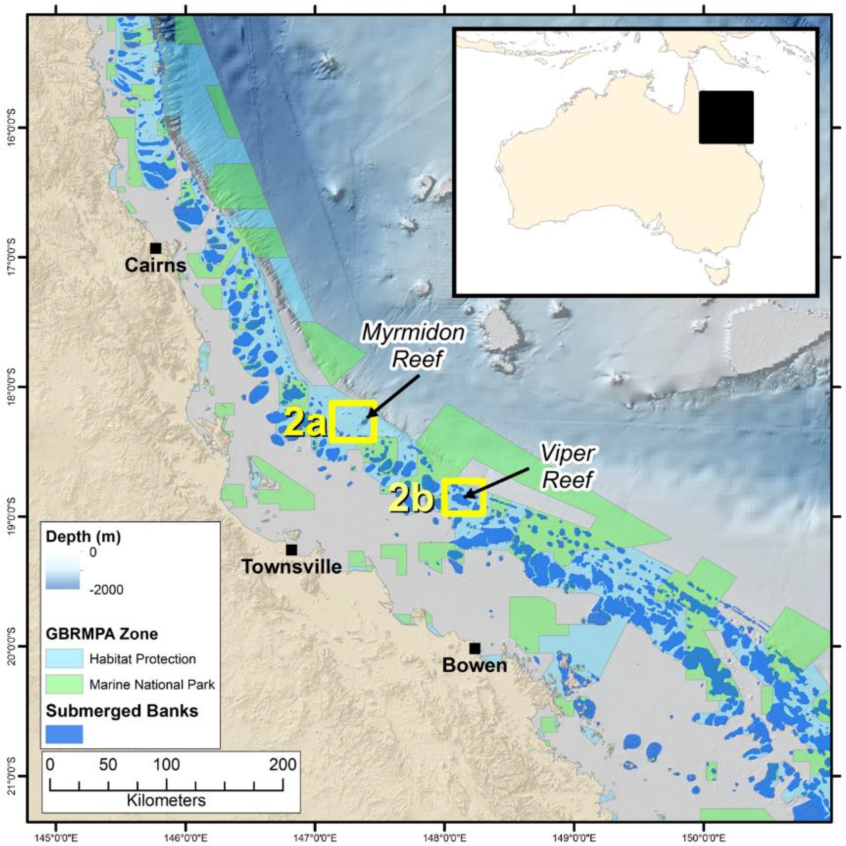
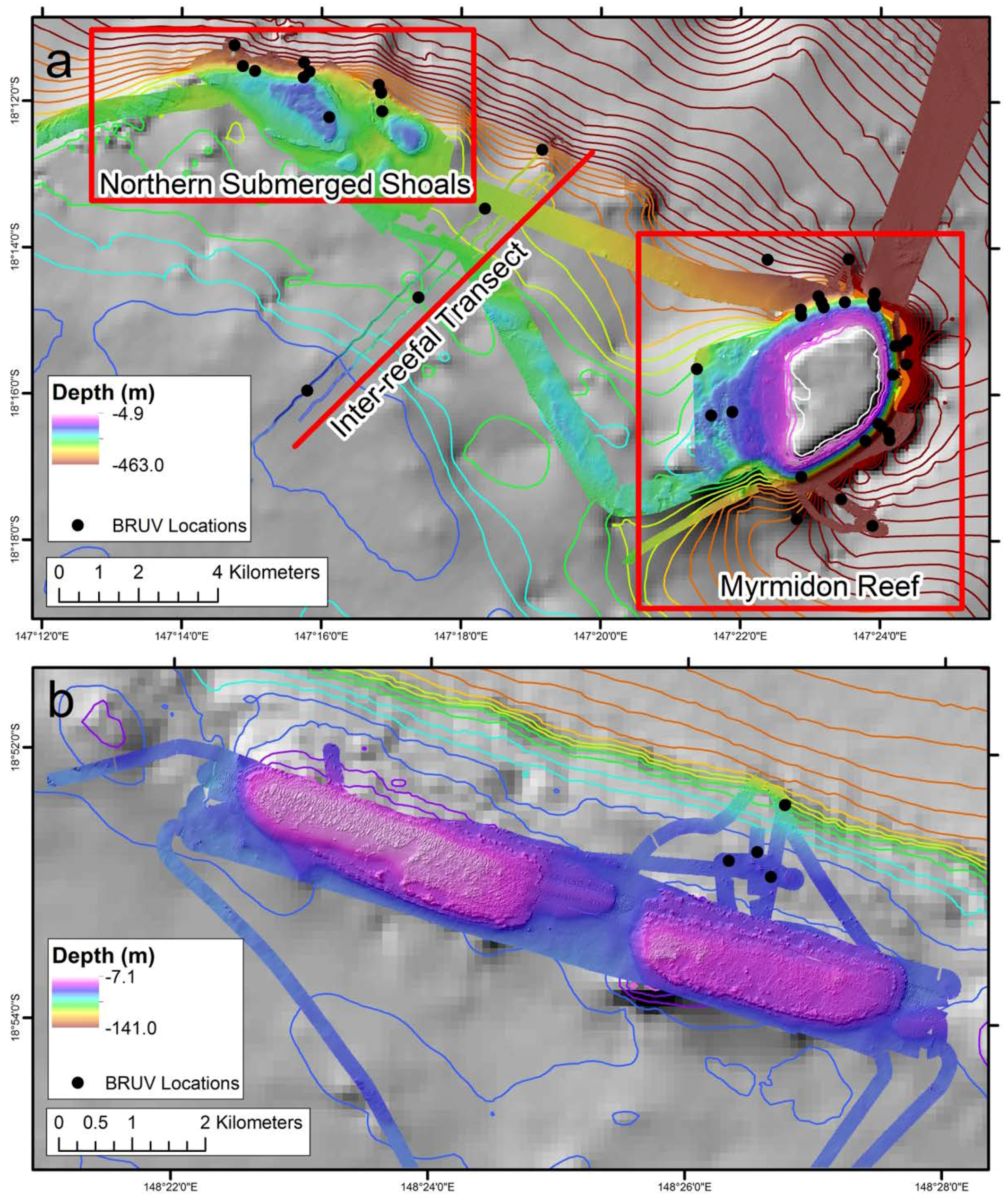
2.1. Study Locations

Submerged shoals along the margin of the GBR support a wide range of ecosystems, largely due to the diverse range of shelf-edge reef morphologies that occur [63]. The central GBR is particularly morphologically distinctive (Figure 1, [64]). In this region, very few major reefs reach sea-level within eight kilometers landward of the shelf-edge, and only one emergent reef is found on the edge itself (Myrmidon Reef, [64]). The shelf-edge here is characterized by one to three lines of submerged reefs, which indicates periods of active development during lower historical sea levels [65]. The central GBR shelf-break is located >100 km from shore, which is a greater distance than in the northern GBR (north of Cairns), but much less than the southern GBR (up to 250 km). Gradients on the upper continental slope in the central GBR are also comparatively low compared to the northern GBR, with a combination of subsidence [66] and sediment input [67] as the likely drivers for this morphology. The region commonly experiences nutrient enrichment as the seasonal thermocline of the adjacent Coral Sea shallows [68], which, in turn, transports nutrient-rich waters to the continental shelf [69].
In order to assess variation in habitats along the upper continental slope environment, four distinct shelf-edge locations were targeted using the multibeam sonar and BRUVS: Myrmidon Reef, a suite of unnamed shoals 15 km northwest of Myrmidon (‘Northern Submerged Shoals’), an inter-reef transect (Figure 2a), and two submerged shoals 30 km east of the Viper Reef (‘Viper Reef’, Figure 2b). The mesophotic benthic communities of the central GBR are composed of a diverse range of habitat-forming taxa such as hard and soft corals (including Scleractinia, zooxanthellate, and azooxanthellate Octocorallia), sponges, seagrasses, and algae [70,71]. Hard substratum above ~60 m is typically dominated by shallow-water zooxanthellate corals such as Montipora, Porites, Seriatopora, and Xeniidae. However, below 60 m, the communities are increasingly dominated by azooxanthellate octocorals [39,72]. Inter-reefal habitats between 50–80 m are generally composed of either bare sand or dense fields of calcareous Halimeda macroalgae, with this species becoming sparse below 80 m in the central GBR [71] but present down to 100 m in the northern GBR [63], and where shelf-edge bathymetry allows nutrient upwelling to occur [73]. The shelf-edge between 90–140 m includes extensive hard reef substratum formed during lower Pleistocene sea levels that now supports dense forests of gorgonians [39,74]. Beyond 140 m, this hard reef substratum is less abundant, with a correlated decline in the abundance of octocorals and other habitat-forming species. The one exception may be the eastern side of the Myrmidon Reef, where a steep rocky slope extends to depths well below 150 m and continues to support azooxanthellate octocorals (T. Bridge pers. obs. from this study).
Within the Great Barrier Reef Marine Park (GBRMP), locations have varying levels of protection based on the activities that are permitted. Approximately 33% of the area is designated Marine National Park Zone as ‘no-take’, where fishing is not allowed [75]. Other zone types occur within the GBRMP. However, the locations included in this study are all under habitat protection, with Myrmidon Reef the only location in a ‘no-take’ zone.

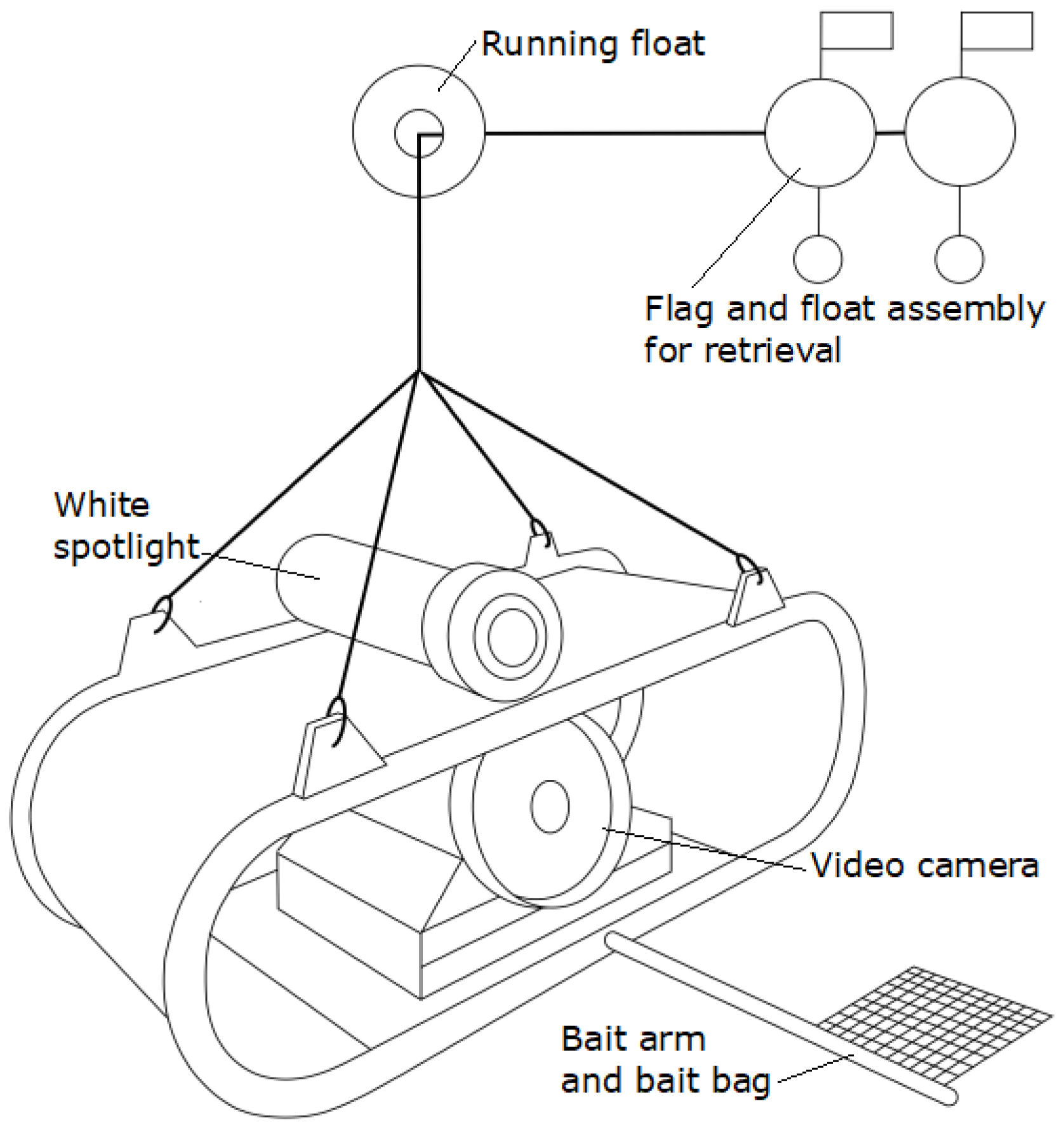
2.2. Baited Remote Underwater Video Stations (BRUVS)

To sample fish assemblages and habitats in situ, 48 single BRUVS deployments were conducted over three research cruises (May, June, and September 2014), all during daylight hours (0700–1800). BRUVS were depth-stratified targeting depths of ~100 m, ~150 m, and over 200 m to investigate depth gradients. Since Viper Reef has the shallowest slope environment, some deployments were placed at depths <100 m to ensure similar width of spacing between BRUVS at the other locations. All BRUVS were set at a minimum distance of 200 m between units to minimize the effects of bait plumes and reduce the likelihood of fish being re-sampled [76]. BRUVS were deployed at sites between 54 to 260 m depth and sampling a total of three reefs and one inter-reefal transect (Figure 2).
A high-definition camera (Sony HDR-CX110E) was housed in an aluminum rollbar-frame for protection during deep deployments while also minimizing damage to benthic habitats (Figure 3). The field-of-view (FOV) of each BRUVS was illuminated by a white spotlight (550 lumen) to overcome diminished light with depth and aid in species identification. The camera focus was set to manual infinity to maximize the FOV. BRUVS were attached to a bridled rope configuration with sufficient rope (8-mm diameter polypropylene, approximately twice the water depth of the deployment because of the strong currents), ballast weights, and a float-flag assembly for retrieval. A plastic mesh bag filled with one kilogram of crushed pilchards (Sardinops sagax) was attached to the BRUVS via a flexible plastic conduit as an attractant. BRUVS were left to soak for 45 min, but, due to the time to reach the bottom, tapes were an average of 54 min (27 to 84 min). BRUVS units were retrieved from the surface using a hydraulic pot-hauler.
Videos were read to the full length, then standardized for number of fishes per hour, using purpose-built software developed by the Australian Institute of Marine Science (AIMS). Fishes were identified to the lowest possible taxonomic level with the help of multiple ichthyologists via correspondence. Time on the seabed, visibility, time of first appearance of each species, abundance N of each species until the time when MaxN was reached (i.e., the greatest number of individuals of a species per frame [51]), and time of the end of sampling (i.e., when the video left the bottom or when the video camera stopped recording) were recorded. Video stills of all fish identified were indexed for inclusion in the AIMS reference image library. MaxN is a conservative estimate of abundance and is used to avoid recounting individuals that exit and re-enter the FOV [77] and provides a minimum estimate of true abundance [78]. Species richness and total abundance were added for each deployment and standardized by effective sampling time to be estimates per hour filmed at the seabed. Individual BRUVS deployments were treated as independent sites and the sites sampled were divided into four locations (Myrmidon Reef, Viper Reef, Northern Submerged Shoals, and the inter-reefal transect).
We hypothesized that some components of the epibenthos and substratum would affect the fish community composition. Benthic habitat information at each site was estimated from the FOV. This included identifying major abiotic and biotic habitat characteristics based on a standardized, tripartite, benthos classification scheme developed for a project that used similar methods to describe patterns in fish and fauna of deeper shoals on the GBR continental shelf with a range of habitat, spatial, and temporal variables [79]. Substratum categories used were bedrock, boulder, calcareous reef, mud/silt, gravel (2–64 mm), rubble, sand, and ‘indeterminate’ (i.e., where substratum could not be determined reliably due to the angle or visibility of the FOV). Bedform categories included qualitative descriptors such as bioturbated sand, boulder field, sand dunes, sand ripples, rubble field, flat gravel/sand/silt, Halimeda beds, high-relief reef, and low-outcrop reef. Benthic community categories included coral, gorgonian, and sea-whip garden, low-relief rubble field, macroalgae bed, open sandy seabed, and seagrass bed. In addition, the following benthic community components were also qualitatively summarized in the same way: anemones, bryozoans/encrusting animals, coralline algae, gorgonian fans, forams, Halimeda, hard coral, hydroids, macroalgae, seagrass, soft coral, sponges, sea whips, zoanthids, and ‘none.’ Each component was given a percentage score 0–100 in increments of 10. Rarer categories of substratum or epibenthos were pooled with related categories for fewer covariates (Table 1).

2.3. Multibeam Sonar Acquisition

Reef architecture can affect the distribution of fishes. For this reason, we obtained a broader suite of information on the underlying habitat structure of shelf-break environments, with multibeam bathymetry and backscatter information describing a number of neighborhood characteristics. High-frequency multibeam sonar produces accurate, high-resolution digital bathymetric models [80]. While this technology is in wide use, it has only recently been applied to study shelf-break reefs and fish communities on the GBR [81,82]. Multibeam information has the potential to characterize fine-scale spatial relationships between deeper habitats and fish [83]. Multibeam echo sounders collect bathymetry and backscatter information over a wide swath of the seafloor [80,84], with the relative acoustic backscatter, i.e., the ‘acoustic reflectivity of the seabed,’ which provides a useful proxy for seabed substratum [84]. Multibeam sonar surveys using a Reson 8101 were conducted in 2014 onboard James Cook University’s RV James Kirby (24, 25 May) and Australian Institute of Marine Science’s RV Cape Ferguson (03–09 Sept). Multibeam mapping in water depths of 10–250 m was conducted at a speed of 5–6 knots. The Reson 8101 emits 101 acoustic beams of 1.5° × 1.5°, covering an angular sector of up to 150° for a total swath approximately seven times the water depth. A Kongsberg Seatex motion reference unit corrected for pitch, roll, and heave. A Fugro OmniSTAR 9200-XP differential GPS recorded positioning, with a quoted accuracy of 1.0 m RMS in the X and Y plane. Data from all peripheral sensors were recorded using QPS QINSy acquisition software. A Sontek CastAway CTD system corrected the acoustic profile. Predicted tides generated from XTide software [85] corrected the bathymetric data by tidal datum over the survey period. Raw multibeam data files were converted to Extended Triton Format (XTF) and imported to Caris HIPS/SIPS post-processing software. All multibeam data post-processing included noise editing, tide, and sound velocity corrections. Bathymetry data were visually inspected and spurious soundings removed to create a level and clean dataset relative to the mean sea level. The error of estimation for vertical soundings reported is estimated to be a maximum of ±0.2 m. The final digital models were produced using Caris HIPS/SIPS software with a 5-m cell size.

2.4. Secondary Datasets from Multibeam

Multibeam sonar datasets measures both the seabed structure through bathymetry and seabed composition with acoustic backscatter [80]. To improve the predictive power of the multibeam sonar datasets, a variety of secondary datasets, potentially correlating with seafloor properties, were produced from the raw bathymetry and backscatter data using neighborhood-based statistics and terrain analysis techniques [84,86]. Neighborhood operations produce an output raster dataset in which each cell location is a function of the input value at a cell location and the values of the cells in a specified kernel (i.e., neighborhood) around that location. The configuration (size and shape) of the kernel determines which cells surrounding the input cell are included in the output value. The most typical kernel size is 3 × 3 cells (i.e., a radius of 1 grid cell), which incorporates the processing cell and its closest eight neighbors.
Multi-scale terrain analysis is predicted to be the most efficient method for characterizing features at multiple spatial scales [86,87,88] and, for this study, we wanted to compare differences between sites on local and broad scales. Derivative datasets that accounted for both high-frequency and low-frequency variations in the multibeam data, and variations in the kernel (neighborhood size), were included in the analyses. All derivatives of the bathymetry and backscatter were chosen because they have a potential influence on the fish community ecology (Table 1) and are commonly used within the marine habitat and seabed characterization (see Reference [89] for a review and Figure S1 for demonstrative examples of backscatter and bathymetry derivatives used in this study). Progressively lower frequency neighborhood analyses were applied to the multibeam bathymetry and backscatter to investigate multiple spatial scales in two ways. Some neighborhood functions (Easting, Northing, Slope, Topographic Position Index, Topographic Ruggedness Index, Surface Ratio, Total Curvature, Planar Curvature, and Profile Curvature) are used to quantify the ‘shape’ of the kernel. As a result, they are calculated from the surrounding eight pixels (a 3 × 3 kernel) and were applied to the bathymetry raster only. Therefore, to achieve progressively ‘lower frequency’ derivatives of these metrics, the bathymetry rasters were low-pass filtered (5 times) using an 11 × 11 kernel-averaging filter. Each time the averaging low-pass filter was applied, the nine neighborhood functions were then calculated to create derivative raster datasets at that resolution (designated ‘**’ in Table 1). Neighborhood functions that could be applied to larger kernel sizes were applied to both the bathymetry and backscatter grids using kernels with radius values of 5 and 50 pixels (Range, Standard Deviation of Bathymetry, Average Backscatter and Standard Deviation of Backscatter, and these multiple spatial scales were designated with ‘***’ in Table 1). Backscatter information can be interpreted as qualities of the substratum (i.e., ‘hard’ or ‘soft’). Raster calculations were undertaken using the R software [90] and the Raster package [91]. Additional subroutines were written for Curvature measurement based on Zevenbergen and Thorne [92]. For site comparisons within depth strata, multibeam information from the 5 × 5 kernel was used, and, for comparisons among depth strata, multibeam derivatives from the 50 × 50 kernel were used.

2.5. Data Analysis

2.5.1. Habitats and Fish Communities Separated by Depth

Depth had a great influence on fish community patterns. However, since numerous ecological factors vary with depth, this can obscure the underlying drivers of fish distributions, including the influence of fish-habitat interactions [62]. Therefore, we investigated habitat differences within and among depth strata. For epibenthic and substratum percent cover comparisons, we divided the sites based on depth categories with n = 16 sites for balance (‘Shallow’ 54–107 m, ‘Middle’ 110–156 m, and ‘Deep’ 160–260 m). We then analyzed patterns of fish and environmental covariates using non-metric multi-dimensional scaling (nMDS) and fitting environmental correlates on the ordination package ‘vegan’ [110] in R. Fish abundance data was divided into ‘Shallow’ (54–115m, n = 18 sites), ‘Middle’ (128–160m, n = 14 sites), and ‘Deep’ (179–260m, n = 12 sites with no missing values) sites and fish species only occurring at one site were removed from the dataset, which left 72 species. Sites (i.e., BRUVS deployments) were eliminated from the analyses if there were missing habitat values (some multibeam values were ‘missing’ if the kernels extended beyond the region where multibeam information was collected, which was more frequent at the deepest sites). One site was removed because it did not contain any of the remaining 72 species. Separating sites into three nMDS investigated the differences in habitats with the maximum separation between depth categories.
Ordination by nMDS separated the sites based on community dissimilarities in relative abundances and composition. Separate nMDS identified what species and habitat variables contributed to similarities among locations (function metaMDS, k = 2). Non-metric MDS is a flexible and robust ordination method for visualizing patterns that preserve the ranks of dissimilarities in species abundance data. Relative abundances were transformed with a fourth-root to reduce the influence of highly abundant fishes and then scaled using a Wisconsin double-standardization with the Hellinger method where species are standardized by the maxima and sites by the site total. Hellinger accounts for relative rarity and the ‘horseshoe effect’ where sites are considered more alike by what species are absent from those sites. Species abundance data were then incorporated into a Bray-Curtis resemblance matrix.
To see what environmental covariates were meaningful for distinguishing sites, correlating covariates were fitted as vectors overlaying the plotted sites if they were above the p < 0.05 significance level (function envfit, Pearson correlations with 999 permutations). This function estimated the strength of the correlation as well as the direction of the correlation among sites. Multibeam information and FOV information were first evaluated for variables that were highly correlated (>0.8) and those variables were removed. The absolute values of multibeam data from the 5 × 5 kernel were log(x+1)-transformed. FOV epibenthic/substratum measurements were arcsine-transformed. Environmental variables were scaled and converted into a Euclidean distance-based matrix.
We also investigated community differences among deep reefs using similarity percentages (SIMPER, PRIMER v7, PRIMER-e, Auckland, New Zealand), which estimated the contributions of fish species to the differences in community composition variability between locations within depth strata. SIMPER analysis used presence/absence-transformed community fish data, using a Bray-Curtis resemblance matrix with 70% as the cut-off level for low contributions.

2.5.2. Species-Species Associations

The occurrence and abundance of fishes may be explained by co-existence or competition with other species in the community. Therefore, we investigated between-species correlations. We plotted significant Pearson correlations (p < 0.05) for all the possible pairs of the 28 most frequently-occurring species using the packages ‘corrplot’ [111] and ‘Hmisc’ (function rcorr, [112]). This subset of 28 species included the relative abundance of fish observed at five or more of the total 48 sites. Significant negative correlations could indicate potentially competing species and significant positive correlations could indicate species co-existing in a similar ecological system.

2.5.3. Trophic Communities

We hypothesized that fishes would have different levels of habitat association and that these levels were likely due to differences in the ecological niche (i.e., what they eat). The degree of habitat specialization between fishes can even be different between closely related species [113,114]. An analysis was conducted to determine differences in the trophic community composition (diversity of feeding groups) between deep-reef habitats. Each species was designated a trophic group based on diet or trophic ecology information, according to Fishbase (herbivore, piscivore, planktivore, general carnivore, benthic carnivore, or unknown [115]). The number of total species per trophic group (presence/absence) per site was summed as a measure of relative trophic richness. Some species’ diets could be inferred to the most likely category based on closely-related species (e.g., Gymnothorax species tend to be carnivores), but, where there were different trophic niches within a family, these species were left as unknown.
Sites were plotted along the two primary axes (PC1 and PC2) accounting for most of the variation in trophic richness using a Principal Component Analysis (PCA) on Wisconsin-standardized trophic group richness. Wisconsin double-standardization first transformed data by ‘species’ maxima and then by ‘site’ totals for a more uniform comparison and common scale among sites with very different numbers of members, reducing the contribution of abundant taxa [116] and improving the gradient detection capability when comparing dissimilarities [117]. Sites were grouped according to the depth category (n = 16, ‘Shallow’ 54–107 m, ‘Middle’ 110–156 m, and ‘Deep’ 160–260 m) and individual habitat measures were correlated to the variance explained in PC1 and PC2. We presumed broad trophic differences would be operating on larger spatial scales, so the multibeam measurements used were from the 50 × 50 kernel (i.e., largest sampling window). This approach compared each single predictor to the combined community response of the principal component. This comparison reduced dimensionality, which increased the ability to identify how much communities respond directly to gradients in the environmental factors [118]. This method determined which habitat variables are most important in explaining the variation among sites.
Animal ethics approval was granted by James Cook University (A1808 and A2207).

3. Results

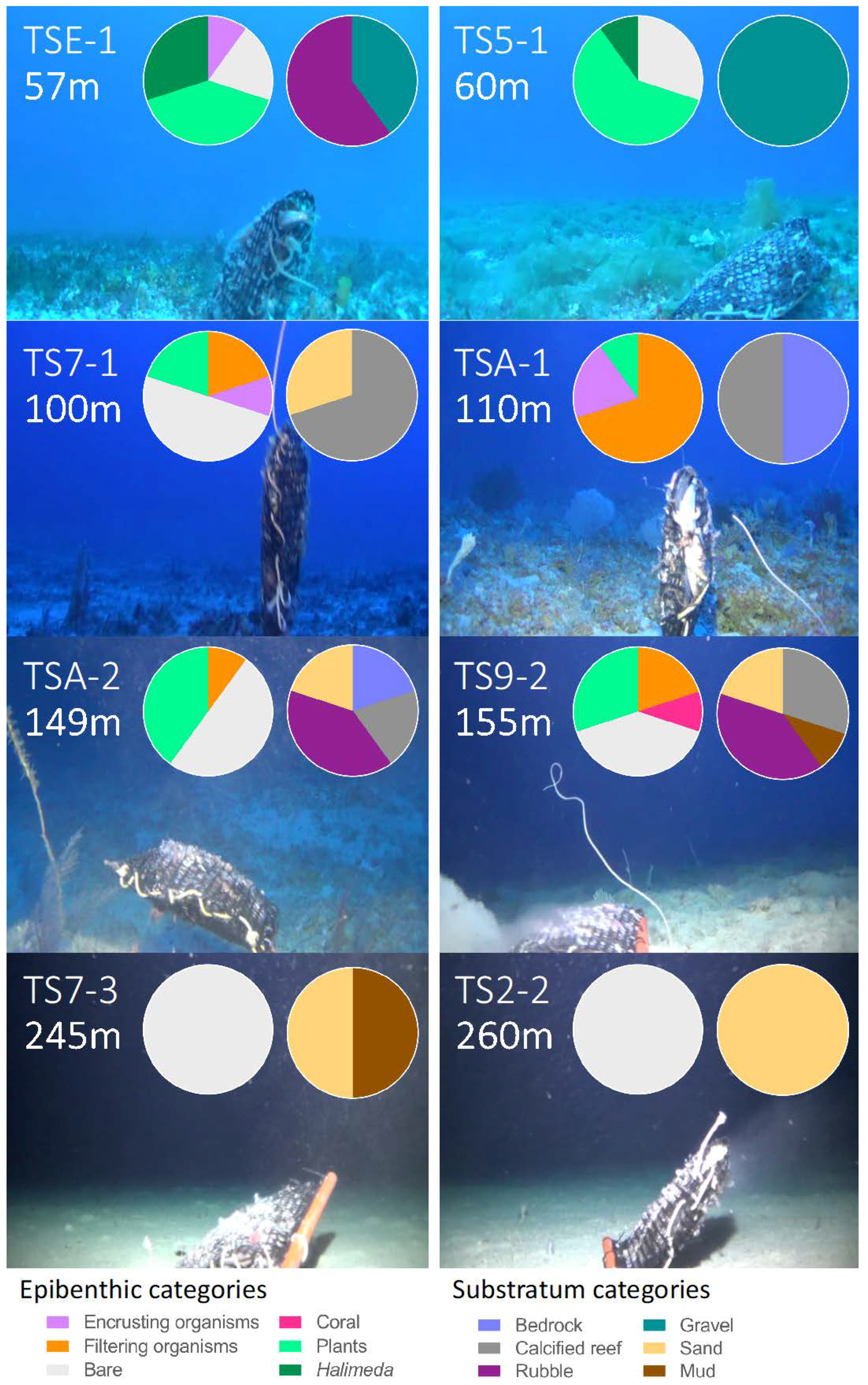
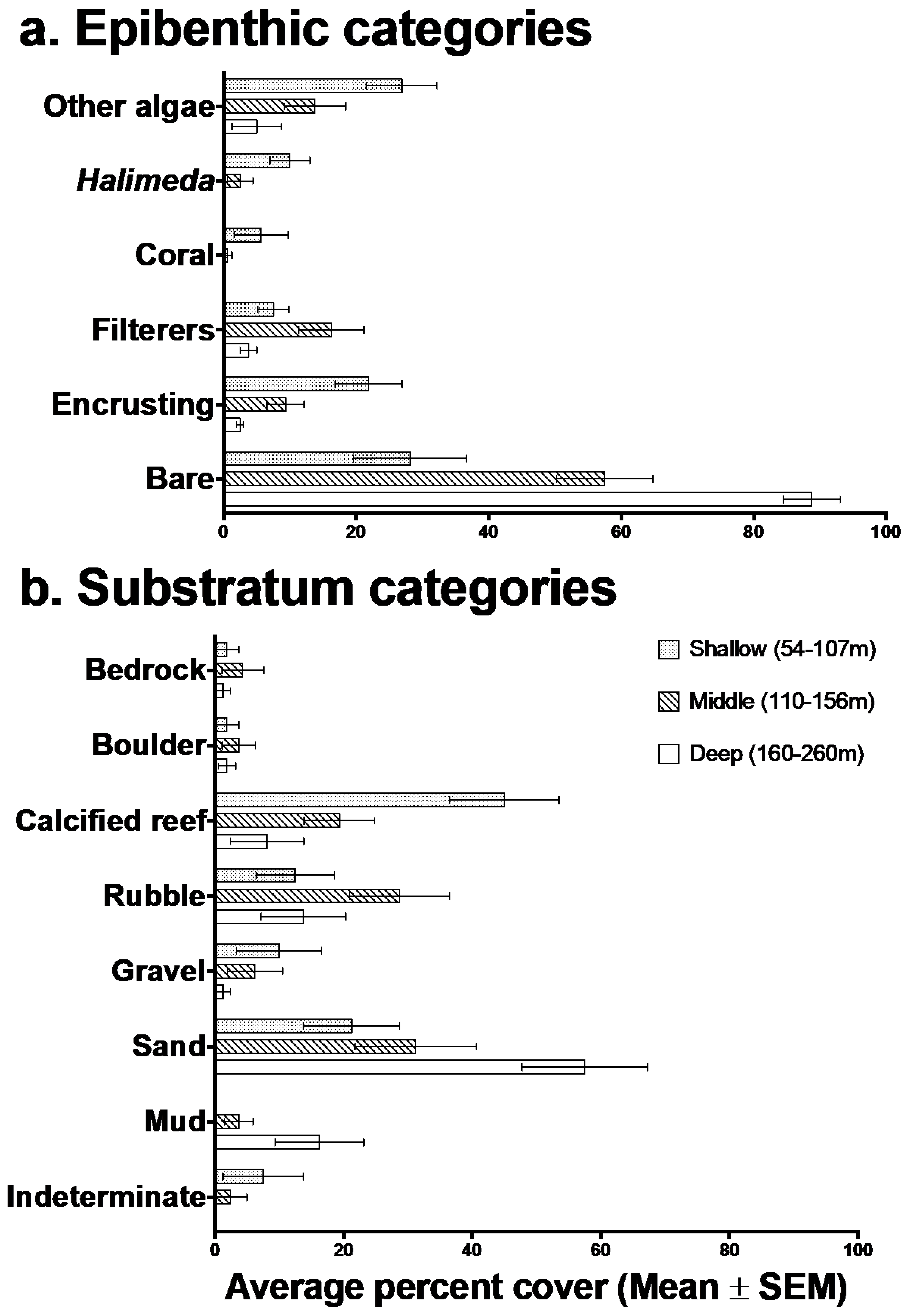
3.1. Description of Deep-Reef Benthic Shelf-Break Habitats

Epibenthic cover and substratum type varied with depth (54–260 m deep, Figure 4 and Figure 5). The mean abundance cover of macro-algae decreased from 27% at the shallowest sites (54–107 m), to 13% at middle sites (110–156 m), to 5% at the deepest sites (160–260 m, Figure 5). Halimeda (kept as a separate category for analyses) was also most prominent in shallower sites (10% mean abundance cover) and was found to a maximum depth of 150 m. Soft corals were seen down to 155 m. Sponges had the greatest representation in the Middle sites (4%–16% average cover). The encrusting community (coralline algae and bryozoans) was most abundant at Shallow sites (~22% mean abundance cover) and decreased with increasing depth. Overall, the average percent cover of the total epibenthic community decreased from Shallow (72%), Middle (43%) to Deep sites (11%), with deeper sites having noticeably more ‘bare’ coverage (89%). Structural complexity also decreased with greater depth, largely due to the declining abundance of calcified reef (mean 45%, 54–107 m, 8%, 160–260 m). However, other hard substratum categories, such as bedrock and boulder, had limited but relatively consistent average abundance cover (1%–4%). Rubble and sand became more common with increasing depth, while mud only appeared in the middle and deeper sites.
There was some notable habitat variation among locations surveyed and also at the level of sites within locations (Figure 4). Overall, epibenthic composition was more similar between Myrmidon Reef and Northern Submerged Shoals than the Viper Reef (Figure S2). While coral was observed at shallow Viper Reef sites, it was absent from other locations (Viper included some shallower sampling depths). In addition, while the abundance of sponges was consistent between the Myrmidon Reef and Northern Submerged Shoals, they were absent from Viper Reef. Macro-algae was abundant at deeper sites of the Northern Submerged Shoals, occurring at three of the four sampling sites and down to 194 m. There were no major differences in substratum by location (Figure S3), but what was visible in the FOV were coarse qualifications of substratum. The number of replicate sites per reef and depth varied (e.g., for inter-reefal sites, there was only one site per depth category), and, therefore, due to low replication at some locations, these results were not analyzed by parametric tests by location.

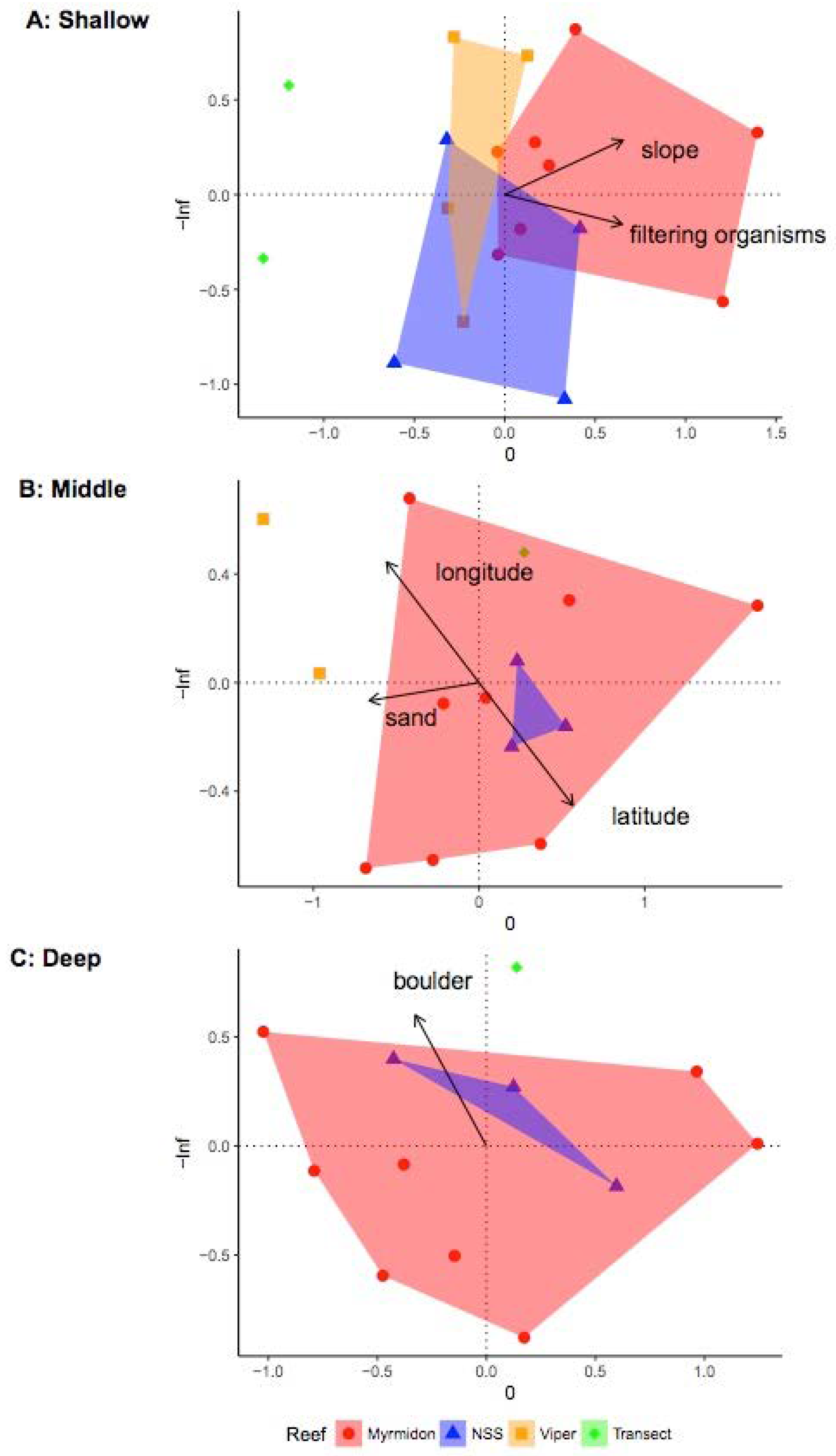
3.2. Investigating Habitats and Fish Communities within Depth Strata

There was great variation in species composition both among locations and sites nested within locations. The differences among locations were greatest at shallow depths, but there was still an overlap between sites among locations (Figure 6). Of the environmental variables responsible for differences among sites, only a few were significant by depth strata. Slope and the presence of filter-feeding organisms among shallow sites were significant (p < 0.05), while Middle sites had the significant separation based on longitude, latitude, and the proportion of sand. The presence of boulder substratum differentiated among sites at Deep sites.
Variation within depth strata show some overall patterns between fish communities by location (Figures S4–S6). Many species are shared among multiple locations, such as Lethrinus rubrioperculatus, Aprion virescens, Gymnocranius euanus, and Carcharhinus albimarginatus, indicated by the close clustering of species towards the middle of the ordination (Figure S4). Among Middle sites, the species composition at Northern Submerged Shoals overlapped with Myrmidon sites, and Viper varied the most in species composition (Figure S5). For the within-location similarity between sites, SIMPER analysis showed the species that contributed to each location’s community were varied and there were also high levels of unexplained variation within depth strata among locations (Table 2). The species showing greater similarities within a location were often representatives of the Lutjanidae, Lethrinidae, Carcharhinidae, and Carangidae families. At Shallow sites, locations sampled were dissimilar in species assemblages because of high species diversity, with the greatest dissimilarities between the inter-reefal transect and the other reefs sampled. Among sites at Middle depths, Myrmidon and Northern Submerged Shoals were the most similar.

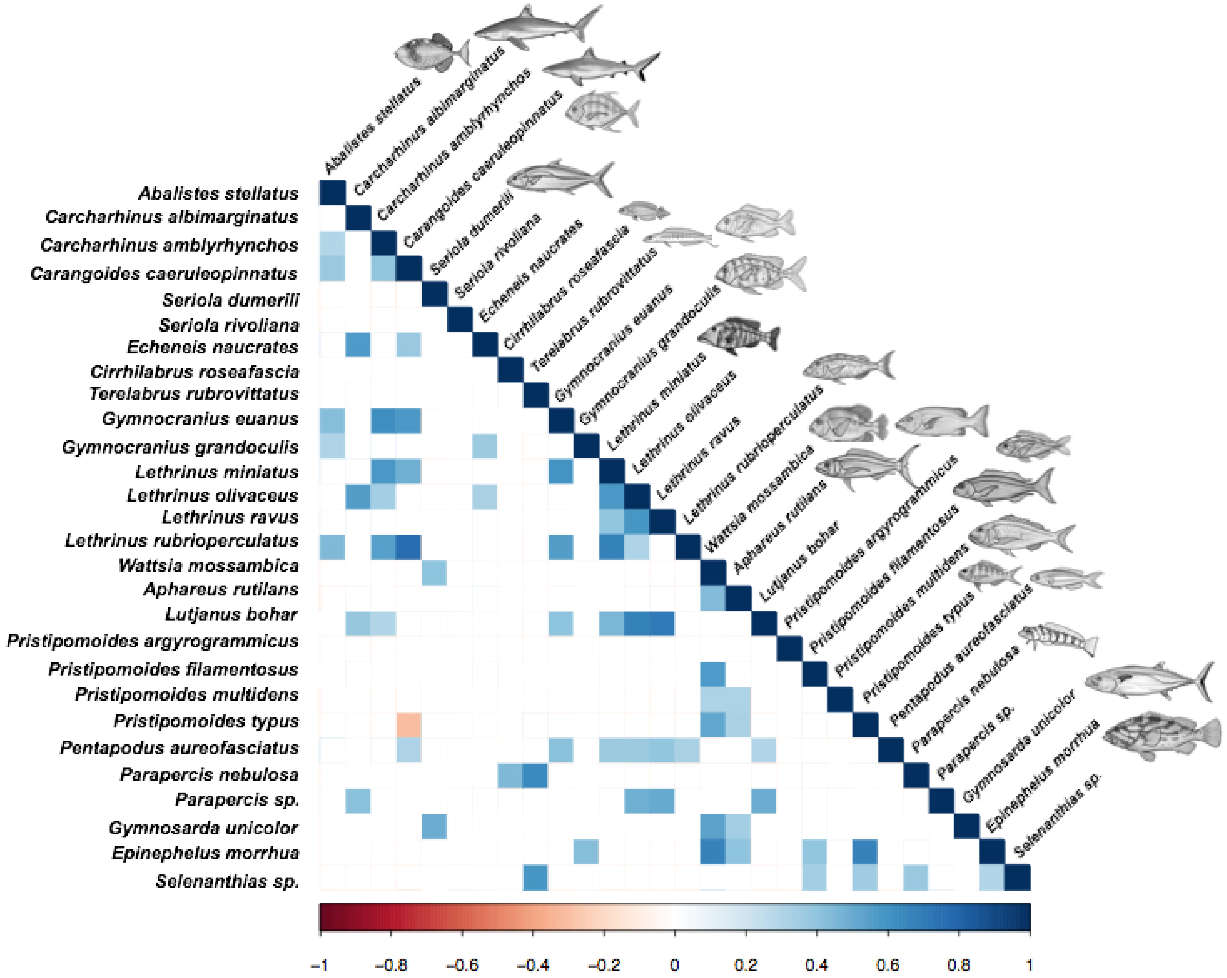
3.3. Relationships among Fish Species

The distribution of fishes among habitats may be both positively and negatively influenced by inter-species interactions. Of the 28 species present at five or more sites, many correlated species were identified (Figure 7 and Figure 8, correlation values with a significance of p < 0.05). L. bohar abundance was highly correlated with the abundance of L. ravus (0.71) and L. olivaceus (0.67), and moderately correlated to Parapercis sp. (0.50, Family Pinguipedidae). Deeper reefs often had mixed groups of lethrinid species: L. olivaceus was often found with L. ravus (0.59) and L. miniatus (0.57); L. miniatus was associated with L. rubrioperculatus (0.68), G. euanus was often frequented seen with species L. rubrioperculatus (0.55) and L. miniatus (0.60). Lethrinid and other family co-occurrences were common: L. rubrioperculatus and C. caeruleopinnatus (0.77), G. euanus with C. caeruleopinnatus (0.58) or the grey reef shark, C. amblyrhynchos (0.62), which also was frequently seen with L. rubrioperculatus (0.54) and L. miniatus (0.57). The silvertip shark, C. albimarginatus, was often seen with an attached sharksucker, E. naucrates (0.57). The deep-reef serranid Epinephelus morrhua and P. typus were frequently observed at the same sites (0.67). W. mossambica was weakly correlated in abundance to deepwater lutjanids P. typus (0.51), and P. filamentosus (0.57), as well as E. morrhua (0.67), and G. unicolor (0.54, Scombridae). Deep reefs commonly featured Parapercis species. P. nebulosa and the labrid, Terelabrus rubrovittatus, were often seen on the same videos and Parapercis sp. abundance was weakly correlated with L. ravus abundance (0.51). T. rubrovittatus was also frequently seen with an unknown Selenanthias sp. (a potential new species for the GBR, 0.59).

3.4. Deep-Reef Fish Trophic Communities

The reef fishes detected in this study were ecologically diverse. Of the 98 fishes identified to species-level, piscivores (10 species), planktivores (7 species), benthic-associated carnivores (26 species), generalist carnivores (41 species), and four species of combined diets (e.g., planktivorous and piscivorous fishes) were represented, based on the membership of known trophic guilds (Table S1 includes species-specific CAAB code [119]). Twenty species recorded had no published trophic information (according to the Fishbase). However, half of these were assigned to a trophic group based on other family members occupying that same trophic group. Only one species was herbivorous (Acanthurus xanthopterus), which is likely due to the decreased availability of edible algae with depth, or the amount of feeding activity around the BRUVS. PC1 and PC2 accounted for a combined 52.5% of the variation among sites, with the presence of general carnivores against the other trophic guilds accounting for the greatest separation and approximately 30% of the total variation (Figure 9). Shallower sites tended to have a greater variety of feeding modes and less overlap with the other depth categories. However, overall, there was a great degree of trophic overlap, especially between the middle and deeper sites (110–260 m).
Several environmental variables were found to have an influence on trophic diversity across PC1 and PC2 (Table S2). Depth, aspect (orientation), planar curvature, and surface ratio dimensions contribute toward the differences in communities along PC1. Fish communities were affected by the local topography and habitat position, presumably because some habitats will be cliff-like features facing the prevailing currents. Proportional measures of bare, plants, bedrock, calcified reef, and presence of sand also correlated with differences along PC1. Slope and standard deviation of the bathymetry were found to explain the variation in PC2.

4. Discussion

Habitat type varied with depth and within depth strata. These differences in reef architecture and benthic cover affected both community and trophic composition of fish communities. While the shelf-break sites sampled all exhibited a steep vertical gradient, individual habitats were highly heterogenous, which varied in both biotic and abiotic characteristics. These factors influenced the distribution and abundance of many fish taxa, as well as broad trophic groups. Many habitat differences corresponded with increasing depth, which is likely driven by vertical variation in temperature, light, and pressure. However, habitats also varied within depth strata with regard to the benthic community composition and underlying substrate type. Most multibeam variables did not correlate with changes in overall fish community composition even though a few (slope, aspect, planar curvature, and surface ratio) could distinguish sites with different trophic communities. This may be because the measures of habitat from different spatial scales, from relatively small scales with BRUVS (<10 m2) and multibeam derivatives describe broader spatial information (~10–100s m2). Topographical features of the habitat, such as slope angle, aspect (i.e., sites facing prevailing currents), rugosity, and planar curvature (e.g., local ridges or valleys) may contribute to the local availability of food and shelter. Among the shallow-depth and middle-depth sites sampled, the fish community composition at the Viper Reef was clearly distinct from other locations. The Viper was located on a shallower portion of the shelf-break, where the reef bottoms out to a maximum depth of 150 m and the slope is less steep. The maximum extent (i.e., deepest depth) of the reef may account for some of the variability in fish communities [33].
Trophic group composition and structure varied with depth, with a greater trophic diversity at upper mesophotic depths and increasing reliance on general carnivores at the deepest depths. This suggested that the ecology of deeper reef fish communities is fundamentally different from those found at shallower depths. Some previous studies have noted a greater abundance of certain trophic groups, such as piscivores, on outer-shelf reefs along the GBR [120]. However, this is the first assessment of depth-related changes in trophic structure below 50 m. Worldwide, many mesophotic habitats are characterized by low herbivore abundances and high planktivore abundances (e.g., the Red Sea, Puerto Rico, Northwest Hawaiian Islands, Brazil, Main Hawaiian Islands, [8,35,121,122,123,124,125]). While this study identified low numbers of planktivorous and piscivorous species compared to other feeding strategies (7%–10%), this is largely due to the lack of trophic specificity available (some of the species observed had ‘unknown’ feeding modes). Depth-related trophic variation indicates a dramatic shift from shallow reef food-web dynamics to strategies that rely more on plankton and other mobile resources. It has been postulated that mobile invertivores [35,122] and anthiine fishes [126,127] are key links within other mesophotic food webs, and the high proportion of carnivores and piscivores found at mesophotic depths within the GBR suggests similar strategies are operating there. Even within the same species of Stegastes partitus, deeper habitat-associated subpopulations had broader diet niches in those in shallower depths [128]. Future trophic comparisons should include relative measures of trophic-level hierarchy, mobility, and prey size [122], as well as quantifying how reliant these predators are on food sources that originate at shallower depths and use vertical diel movements to target benthic prey [129] if there are ‘trophic subsidies’ in operation where oceanic planktonic and nektonic resources make up the deficit for dwindling primary productivity at deeper depths [130].
Identifying where species co-occur is an important consideration in ecosystem-based fisheries management used to predict the degree that species interact. Species distributions that are highly correlated will also affect fishing mortality estimates in multispecies fisheries [131]. More connected species are thought to have a higher vulnerability to combined anthropogenic threats as well as detrimental changes to the community structure [132]. The species co-occurrences identified in this study suggest the presence of both inter-family and intra-family interactions, similar habitat needs, or greater food availability. However, since the majority of overlapping fish species are upper-level predators, these are likely examples of competition or niche partitioning rather than predator-prey interactions. In addition to differences in trophic groups with depth, there was substantial variation in overall fish community composition both between and within-depths, with this information on variability critical for future management plans. Previous surveys of mesophotic and sub-mesophotic shelf-break reefs suggested species composition is often highly heterogeneous [133] with potentially high proportions of both rare species [134] and endemism [7,135]. New and highly unique fish communities are being frequently described, as mesophotic research effort increases [24,124,136]. Our surveys identified a number of new potential species as well as new location records for the GBR.
Variation in fish community structure among and within depths likely reflects differences in the biotic and abiotic components of shelf-break reefs, with these habitats distinctive from shallower reefs along the continental shelf. A greater proportion of sponges and macro-algae within the benthic community, and the presence of boulders, distinguish shelf-break environments from shallower habitats, as well as differences among shelf-break reef habitats. Not only were significant differences in the community composition found between the sampled reefs, but also between reefs and inter-reefal areas. This is especially true at the shallower depths where a steep slope angle and a high abundance of filter-feeding invertebrates were characterizing features. Sponges and filters are an important habitat-forming component of the upper mesophotic zone along the central GBR [26,137], compared to shallow reefs where coral is the primary ecosystem engineer. Dominant benthic taxa shift from photosynthetic to obligate heterotrophic in deeper, mesophotic Indo-Pacific environments [39,72,138]. The central GBR shelf-break has similar benthic habitats to other clear, tropical mesophotic regions, where Halimeda and corals are observed down to >150 m [37,139,140]. While the lower mesophotic zone is dominated by depth-specialist benthic communities that are distinct from shallower areas [141], coral communities have been documented in transitional depths of 60 to 75 m at multiple sites [39,82]. The lower depth-limits of corals vary, with isolated coral colonies documented to at least 125 m in some locations in the GBR and neighboring Coral Sea [64,142], this study). Halimeda bioherms, while not explicitly studied here, are common macro-algal components of deep reef ecosystems and provide important deposits of calcium carbonate that promotes reef growth. In this study, we observed photosynthetic algae at deeper depths than reported in other MCEs worldwide, which is likely due to well-documented nutrient upwelling. Macro-algal communities in other mesophotic locations have also found new mesophotic-specific species [143,144]. At the deepest depths surveyed, boulders replaced reef-building organisms in creating structural complexity. It is clear that, in the GBR, the shelf-edge should be considered an ecologically unique ecosystem and fundamentally different from shallow reefs, which is similar to other MCEs [24,134,145].
Shelf-break reefs are likely critical habitats for key ecological processes, and it is not yet known to what extent these habitats are necessary for certain species to thrive. Anecdotally, several of the BRUVS deployments observed juvenile fish at mesophotic depths. While it was not always possible to identify juvenile fish to the species-level (and single BRUVS only allow an estimated size), some fish appear to complete most of the life cycle in solely deep habitats, such as the grouper Epinephelus morrhua (Figure 10). In general, the juvenile habitats of the deep-reef species we observed are not well-documented. For instance, juvenile habitats of Pristipomoides sp. were only accidentally discovered over deep (65–100 m), flat, soft habitats in Hawaii [146]. Dogtooth tuna, Gymnosarda unicolor, were observed in groups of 1–3 in all BRUVS deployments except one (Figure 10c). This behavior could be a spawning aggregation, to increase safety from predators, or to increase hunting success. Certain Lutjanidae and Serranidae spawning aggregations are reliable and infamous worldwide [147,148,149]. The use of different habitats by many species to complete their life cycle is not known for the GBR, and future research should attempt to describe and quantify how deep reefs are important for spawning, ontogenetic shifts and life history cycles.

5. Conclusions

This study has shown that benthic composition can influence the distribution and abundance of mesophotic fish communities. Therefore, further research on the distribution and composition of deep-reef habitats is critical to understanding mesophotic biodiversity. A greater sampling effort of the GBR shelf-break along its latitudinal extent would fill in existing knowledge gaps on these deeper marine biomes and would be useful for future conservation strategies. When the GBR Marine Park (GBRMP) protection and mixed-use zonation was determined a decade ago, only coarse environmental data was available for the deeper habitats within the GBRMP [10]. The strategy of the conservation zones allowed for some uncertainty and was designed to protect unknown habitats [75], and incidentally ~30% of submerged banks are within no-take areas and 88% of banks are protected from bottom-trawling [10,150]. Of the locations sampled, only Myrmidon is afforded greater protection as a ‘no-take’ area with the other locations under habitat protection. However, this research showed community differences between reefs and also between reefal and inter-reefal sites. In the future, it will be important to compare species richness and abundance over different protection levels and to include inter-reefal areas for habitat protection, since currently there is no information if existing habitat protection measures are sufficient to safeguard deep-reef fish communities. More detailed benthic habitat mapping and biotic surveys have improved the representative distributions of habitats and fishes in other marine conservation parks in Australia [96,151]. Therefore, increasing the understanding of GBR shelf-break habitats should be a priority. While BRUVS have some biases and limitations, such as the effects of light, bait, and the field-of-view, BRUVS proved to be useful for gaining a better understanding of deep-reef fish communities and habitats. The species composition of fishes varied greatly among habitats. Although depth was important, habitat preferences clearly had a role in determining the distribution of species and trophic groups. Potential predictors of fish distributions on the shelf-break are depth, reef architecture, and benthic cover. The narrow spatial extent of the mesophotic areas on the GBR and other locations makes them vulnerable to fisheries.

Supplementary Materials

The following are available online at https://www.mdpi.com/1424-2818/11/2/26/s1, Figure S1: Examples of multibeam bathymetry, backscatter and derivatives for the Northern Submerged Shoals Figure S2: Epibenthic habitat measures by reef, Figure S3: Substratum habitat measures by reef, Figure S4: Non-metric multidimensional scaling showing fish community composition for Shallow sites (54–115 m), Figure S5: Non-metric multidimensional scaling showing fish community composition for Middle sites (128–160 m), Figure S6: Non-metric multidimensional scaling showing fish community composition for Deep sites (179–260 m); Table S1: Ecology of deep-reef fishes seen in deep Baited Remote Underwater Video Stations, Table S2: Habitat variables to understand variation in fish trophic communities.

Author Contributions

Conceptualization, T.L.S., J.J.D., T.C.L.B., R.J.B., M.C., and M.J.K. Methodology, T.L.S., J.J.D., M.C., and M.J.K. Software, T.L.S., J.J.D., and M.C. Validation, J.J.D. and M.C. Formal Analysis, T.L.S. and J.J.D. Investigation, T.L.S., J.J.D., and T.C.L.B. Resources, T.L.S., J.J.D., R.J.B., and M.C. Data Curation, J.J.D., R.J.B., and M.C. Writing—Original Draft Preparation, T.L.S., J.J.D., and T.C.L.B. Writing—Review & Editing, T.L.S., M.C., R.J.B., J.J.D., T.C.L.B., and M.J.K. Visualization, J.J.D. and T.L.S. Supervision, M.J.K., M.C., and R.J.B. Project Administration, M.J.K., T.L.S., J.J.D., and T.C.L.B. Funding Acquisition, T.L.S., J.J.D., T.C.L.B., and M.J.K.

Acknowledgments

Thank you to the captain and crews of the R/V James Kirby and R/V Cape Ferguson and to fieldwork volunteers: L. Currey, J. White, R. Brooker, A. Thompson, M. Ireland, M. O’Callaghan, T. Manoy, H. Epstein, H. Welch, and S. Kingsford. Special thanks to M. Stowar, M. Wakefield, and P. Speare for logistical support at AIMS and aboard the R/V Cape Ferguson. IT and database support from G. Ericson and E. Johansson. Statistical coaching from M. Logan (AIMS). This research would not have been possible without funding from: ARC Center of Excellence for Coral Reef Studies (M.J.K.), GBRMPA Science for Management Award (T.L.S.), Holsworth Wildlife Research Fund (T.L.S.), PADI Foundation (T.L.S.), JCU Across Boundaries (J.J.D. and T.L.S.), Great Barrier Reef Foundation Bommies Award (T.L.S.), Australian Coral Reef Society Terry Walker Prize (T.L.S.), and support from AIMS@JCU and the Australian Institute of Marine Science (T.L.S.). In memory of M. Cunningham.

Conflicts of Interest

The authors declare that there are no conflict of interest.

References

  1. Lindfield, S.J.; Harvey, E.S.; Halford, A.R.; McIlwain, J.L. Mesophotic depths as refuge areas for fishery-targeted species on coral reefs. Coral Reefs 2016, 35, 125–137. [Google Scholar] [CrossRef]
  2. Garcia-Sais, J.R. Reef habitats and associated sessile-benthic and fish assemblages across a euphotic–mesophotic depth gradient in Isla Desecheo, Puerto Rico. Coral Reefs 2010, 29, 277–288. [Google Scholar] [CrossRef]
  3. Feitoza, B.M.; Rosa, R.S.; Rocha, L.A. Ecology and zoogeography of deep-reef fishes in northeastern Brazil. Bull. Mar. Sci. 2005, 76, 725–742. [Google Scholar]
  4. Jorgensen, S.J.; Klimley, A.P.; Muhlia-Melo, A.F. Scalloped hammerhead shark Sphyrna lewini, utilizes deep-water, hypoxic zone in the Gulf of California. J. Fish Biol. 2009, 74, 1682–1687. [Google Scholar] [CrossRef]
  5. Hoyos-Padilla, E.M.; Ketchum, J.T.; Klimley, A.P.; Galván-Magaña, F. Ontogenetic migration of a female scalloped hammerhead shark Sphyrna lewini in the Gulf of California. Anim. Biotelem. 2014, 2, 17. [Google Scholar] [CrossRef]
  6. Cappo, M.; Kelley, R. Connectivity in the Great Barrier Reef World Heritage Area—An overview of pathways and processes. In Oceanographic Processes of Coral Reefs; CRC Press LLC: Boca Raton, FL, USA, 2010; pp. 161–175. [Google Scholar]
  7. Kane, C.; Kosaki, R.K.; Wagner, D. High levels of mesophotic reef fish endemism in the Northwestern Hawaiian Islands. Bull. Mar. Sci. 2014, 90, 693–703. [Google Scholar] [CrossRef]
  8. Bejarano, I.; Appeldoorn, R.; Nemeth, M. Fishes associated with mesophotic coral ecosystems in La Parguera, Puerto Rico. Coral Reefs 2014, 33, 313–328. [Google Scholar] [CrossRef]
  9. Heyns, E.R.; Bernard, A.T.F.; Richoux, N.B.; Götz, A. Depth-related distribution patterns of subtidal macrobenthos in a well-established marine protected area. Mar. Biol. 2016, 163, 39. [Google Scholar] [CrossRef]
  10. Bridge, T.C.L.; Grech, A.M.; Pressey, R.L. Factors influencing incidental representation of previously unknown conservation features in marine protected areas. Conserv. Biol. 2016, 30, 154–165. [Google Scholar] [CrossRef]
  11. Harborne, A.R.; Mumby, P.J.; Kennedy, E.V.; Ferrari, R. Biotic and multi-scale abiotic controls of habitat quality and their effect on coral-reef fishes. Mar. Ecol. Prog. Ser. 2011, 437, 201–214. [Google Scholar] [CrossRef]
  12. Friedlander, A.M.; Parrish, J.D. Habitat characteristics affecting fish assemblages on a Hawaiian coral reef. J. Exp. Mar. Biol. Ecol. 1998, 224, 1–30. [Google Scholar] [CrossRef]
  13. Choat, J.; Ayling, A. The relationship between habitat structure and fish faunas on New Zealand reefs. J. Exp. Mar. Biol. Ecol. 1987, 110, 257–284. [Google Scholar] [CrossRef]
  14. Yoklavich, M.M.; Greene, H.G.; Cailliet, G.M.; Sullivan, D.E.; Lea, R.N.; Love, M.S. Habitat associations of deep-water rockfishes in a submarine canyon: An example of a natural refuge. Fish. Bull. 2000, 98, 625–641. [Google Scholar]
  15. Stein, D.L.; Tissot, B.N.; Hixon, M.A.; Barss, W. Fish-habitat associations on a deep reef at the edge of the Oregon continental-shelf. Fish. Bull. 1992, 90, 540–551. [Google Scholar]
  16. Majewski, A.; Atchison, S.; MacPhee, S.; Eert, J.; Niemi, A.; Michel, C.; Reist, J.D. Marine fish community structure and habitat associations on the Canadian Beaufort shelf and slope. Deep Sea Res. Part I Oceanogr. Res. Pap. 2017. [Google Scholar] [CrossRef]
  17. MacNeil, M.A.; Connolly, S.R. Multi-scale patterns and processes in reef fish abundance. In Ecology of Fishes on Coral Reefs; Mora, C., Ed.; Cambridge University Press: Cambridge, UK, 2015; pp. 116–124. [Google Scholar]
  18. Connell, S.; Jones, G. The influence of habitat complexity on postrecruitment processes in a temperate reef fish population. J. Exp. Mar. Biol. Ecol. 1991, 151, 271–294. [Google Scholar] [CrossRef]
  19. Heck, K.L.; Orth, R.J. Seagrass habitats: The roles of habitat complexity, competition and predation in structuring associated fish and motile macroinvertebrate assemblages. In Estuarine Perspectives; Elsevier: Amsterdam, The Netherlands, 1980; pp. 449–464. [Google Scholar]
  20. Johnson, D.W. Predation, habitat complexity, and variation in density-dependent mortality of temperate reef fishes. Ecology 2006, 87, 1179–1188. [Google Scholar] [CrossRef]
  21. Messmer, V.; Jones, G.P.; Munday, P.L.; Holbrook, S.J.; Schmitt, R.J.; Brooks, A.J. Habitat biodiversity as a determinant of fish community structure on coral reefs. Ecology 2011, 92, 2285–2298. [Google Scholar] [CrossRef]
  22. Alvarez-Filip, L.; Dulvy, N.K.; Gill, J.A.; Côté, I.M.; Watkinson, A.R. Flattening of Caribbean coral reefs: Region-wide declines in architectural complexity. Proc. R. Soc. B Biol. Sci. 2009, 276, 3019. [Google Scholar] [CrossRef]
  23. Graham, N.A. Habitat complexity: Coral structural loss leads to fisheries declines. Curr. Biol. 2014, 24, R359–R361. [Google Scholar] [CrossRef]
  24. Rocha, L.A.; Pinheiro, H.T.; Shepherd, B.; Papastamatiou, Y.P.; Luiz, O.J.; Pyle, R.L.; Bongaerts, P. Mesophotic coral ecosystems are threatened and ecologically distinct from shallow water reefs. Science 2018, 361, 281–284. [Google Scholar] [CrossRef]
  25. Andradi-Brown, D.; Laverick, J.; Bejarano, I.; Bridge, T.; Colin, P.; Eyal, G.; Jones, R.; Kahng, S.; Reed, J.; Smith, T. Mesophotic Coral Ecosystems—A Lifeboat for Coral Reefs? 2016. Available online: http://www.grida.no/publications/88 (accessed on 20 December 2016).
  26. Fitzpatrick, B.M.; Harvey, E.S.; Heyward, A.J.; Twiggs, E.J.; Colquhoun, J. Habitat specialization in tropical continental shelf demersal fish assemblages. PLoS ONE 2012, 7, e39634. [Google Scholar] [CrossRef]
  27. Sink, K.; Boshoff, W.; Samaai, T.; Timm, P.; Kerwath, S. Observations of the habitats and biodiversity of the submarine canyons at Sodwana Bay: Coelacanth research. S. Afr. J. Sci. 2006, 102, 466–474. [Google Scholar]
  28. Kelley, C.; Moffitt, R.; Smith, J.R. Mega- to micro-scale classification and description of bottomfish essential fish habitat on four banks in the Northwestern Hawaiian Islands. Atoll Res. Bull. 2006, 542, 319–332. [Google Scholar]
  29. Parker, R.; Mays, R. Southeastern US Deepwater Reef Fish Assemblages, Habitat Characteristics, Catches, and Life History Summaries; US Department of Commerce: Washington, DC, USA, 1998.
  30. Starr, R.M.; Green, K.; Sala, E. Deep-water fish assemblages at Isla del Coco National Park and Las Gemelas Seamounts, Costa Rica. Rev. Biol. Trop. 2012, 60, 347–362. [Google Scholar] [CrossRef]
  31. Heyns-Veale, E.R.; Bernard, A.T.F.; Richoux, N.B.; Parker, D.; Langlois, T.J.; Harvey, E.S.; Götz, A. Depth and habitat determine assemblage structure of South Africa’s warm-temperate reef fish. Mar. Biol. 2016, 163, 158. [Google Scholar] [CrossRef]
  32. Thresher, R.E.; Colin, P.L. Trophic structure, diversity and abundance of fishes of the deep reef (30–300 m) at Enewetak, Marshall Islands. Bull. Mar. Sci. 1986, 38, 253–272. [Google Scholar]
  33. Andradi-Brown, D.A.; Gress, E.; Wright, G.; Exton, D.A.; Rogers, A.D. Reef fish community biomass and trophic structure changes across shallow to upper-mesophotic reefs in the Mesoamerican Barrier Reef, Caribbean. PLoS ONE 2016, 11, e0156641. [Google Scholar] [CrossRef]
  34. Brokovich, E.; Einbinder, S.; Shashar, N.; Kiflawi, M.; Kark, S. Descending to the twilight-zone: Changes in coral reef fish assemblages along a depth gradient down to 65 m. Mar. Ecol. Prog. Ser. 2008, 371, 253–262. [Google Scholar] [CrossRef]
  35. Fukunaga, A.; Kosaki, R.K.; Wagner, D.; Kane, C. Structure of Mesophotic Reef Fish Assemblages in the Northwestern Hawaiian Islands. PLoS ONE 2016, 11, e0157861. [Google Scholar] [CrossRef]
  36. Kane, C.N.; Tissot, B.N. Trophic designation and live coral cover predict changes in reef-fish community structure along a shallow to mesophotic gradient in Hawaii. Coral Reefs 2017, 1–11. [Google Scholar] [CrossRef]
  37. Kahng, S.E.; Garcia-Sais, J.R.; Spalding, H.L.; Brokovich, E.; Wagner, D.; Weil, E.; Hinderstein, L.; Toonen, R.J. Community ecology of mesophotic coral reef ecosystems. Coral Reefs 2010, 29, 255–275. [Google Scholar] [CrossRef]
  38. Dennis, G.D.; Bright, T.J. Reef fish assemblages on hard banks in the northwestern Gulf of Mexico. Bull. Mar. Sci. 1988, 43, 280–307. [Google Scholar]
  39. Bridge, T.; Done, T.; Beaman, R.; Friedman, A.; Williams, S.; Pizarro, O.; Webster, J. Topography, substratum and benthic macrofaunal relationships on a tropical mesophotic shelf margin, central Great Barrier Reef, Australia. Coral Reefs 2011, 30, 143–153. [Google Scholar] [CrossRef]
  40. Pyle, R.L. Use of advanced mixed-gas diving technology to explore the coral reef “Twilight Zone”. Ocean Pulse Crit. Diagn. 1998, 71–88. [Google Scholar] [CrossRef]
  41. Cánovas-Molina, A.; Montefalcone, M.; Bavestrello, G.; Cau, A.; Bianchi, C.N.; Morri, C.; Canese, S.; Bo, M. A new ecological index for the status of mesophotic megabenthic assemblages in the Mediterranean based on ROV photography and video footage. Cont. Shelf Res. 2016, 121, 13–20. [Google Scholar] [CrossRef]
  42. McLean, D.L.; Partridge, J.C.; Bond, T.; Birt, M.J.; Bornt, K.R.; Langlois, T.J. Using industry ROV videos to assess fish associations with subsea pipelines. Cont. Shelf Res. 2017, 141, 76–97. [Google Scholar] [CrossRef]
  43. Williams, S.B.; Pizarro, O.; Webster, J.M.; Beaman, R.J.; Mahon, I.; Johnson-Roberson, M.; Bridge, T.C.L. Autonomous underwater vehicle–assisted surveying of drowned reefs on the shelf edge of the Great Barrier Reef, Australia. J. Field Robot. 2010, 27, 675–697. [Google Scholar] [CrossRef]
  44. Starr, R.M.; Fox, D.S.; Hixon, M.A.; Tissot, B.N.; Johnson, G.E.; Barss, W.H. Comparison of Submersible-Survey and Hydroacoustic-Survey Estimates of Fish Density on a Rocky Bank; US Dept. of Commerce, National Marine Fisheries Service: Washington, DC, USA, 1996.
  45. Tissot, B.N.; Hixon, M.A.; Stein, D.L. Habitat-based submersible assessment of macro-invertebrate and groundfish assemblages at Heceta Bank, Oregon, from 1988 to 1990. J. Exp. Mar. Biol. Ecol. 2007, 352, 50–64. [Google Scholar] [CrossRef]
  46. Langlois, T.J.; Fitzpatrick, B.R.; Fairclough, D.V.; Wakefield, C.B.; Hesp, S.A.; McLean, D.L.; Harvey, E.S.; Meeuwig, J.J. Similarities between line fishing and baited stereo-video estimations of length-frequency: Novel application of kernel density estimates. PLoS ONE 2012, 7, e45973. [Google Scholar] [CrossRef]
  47. Johansson, C.; Stowar, M.; Cappo, M. The use of stereo BRUVS for measuring fish size. In Marine and Tropical Sciences Research Facility Report Series; Australian Institute of Marine Science: Cape Cleveland, Australia, 2008. [Google Scholar]
  48. Hannah, R.W.; Blume, M.T. The influence of bait and stereo video on the performance of a video lander as a survey tool for marine demersal reef fishes in Oregon waters. Mar. Coast. Fish. 2014, 6, 181–189. [Google Scholar] [CrossRef]
  49. Harvey, E.S.; Newman, S.J.; McLean, D.L.; Cappo, M.; Meeuwig, J.J.; Skepper, C.L. Comparison of the relative efficiencies of stereo-BRUVs and traps for sampling tropical continental shelf demersal fishes. Fish. Res. 2012, 125–126, 108–120. [Google Scholar] [CrossRef]
  50. Merritt, D.; Donovan, M.K.; Kelley, C.; Waterhouse, L.; Parke, M.; Wong, K.; Drazen, J.C. BotCam: A baited camera system for nonextractive monitoring of bottomfish species. Fish. Bull. 2011, 109, 56–67. [Google Scholar]
  51. Ellis, D.; DeMartini, E. Evaluation of a video camera technique for indexing abundances of juvenile pink snapper, Pristipomoides filamentosus, and other Hawaiian insular shelf fishes. Oceanogr. Lit. Rev. 1995, 9, 786. [Google Scholar]
  52. Whitmarsh, S.K.; Fairweather, P.G.; Huveneers, C. What is Big BRUVver up to? Methods and uses of baited underwater video. Rev. Fish. Biol. Fish. 2017, 27, 53–73. [Google Scholar] [CrossRef]
  53. Cappo, M.; De’ath, G.; Speare, P. Inter-reef vertebrate communities of the Great Barrier Reef Marine Park determined by baited remote underwater video stations. Mar. Ecol. Prog. Ser. 2007, 350, 209–221. [Google Scholar] [CrossRef] [Green Version]
  54. Langlois, T.; Harvey, E.; Fitzpatrick, B.; Meeuwig, J.; Shedrawi, G.; Watson, D. Cost-efficient sampling of fish assemblages: Comparison of baited video stations and diver video transects. Aquat. Biol. 2010, 9, 155–168. [Google Scholar] [CrossRef]
  55. Watson, D.L.; Harvey, E.S.; Fitzpatrick, B.M.; Langlois, T.J.; Shedrawi, G. Assessing reef fish assemblage structure: How do different stereo-video techniques compare? Mar. Biol. 2010, 157, 1237–1250. [Google Scholar] [CrossRef]
  56. Andradi-Brown, D.A.; Macaya-Solis, C.; Exton, D.A.; Gress, E.; Wright, G.; Rogers, A.D. Assessing Caribbean shallow and mesophotic reef fish communities using Baited-Remote Underwater Video (BRUV) and Diver-Operated Video (DOV) survey techniques. PLoS ONE 2016, 11, e0168235. [Google Scholar] [CrossRef]
  57. Cappo, M. Development of a Baited Video Technique and Spatial Models to Explain Patterns of Fish Biodiversity in Inter-Reef Waters. Ph.D. Thesis, James Cook University, Townsville, Australia, 2010. [Google Scholar]
  58. Espinoza, M.; Cappo, M.; Heupel, M.R.; Tobin, A.J.; Simpfendorfer, C.A. Quantifying shark distribution patterns and species-habitat associations: Implications of marine park zoning. PLoS ONE 2014, 9, e106885. [Google Scholar] [CrossRef]
  59. Harvey, E.; McLean, D.; Frusher, S.; Haywood, M.; Newman, S.; Williams, A. The Use of BRUVs as a Tool for Assessing Marine Fisheries and Ecosystems: A Review of the Hurdles and Potential; University of Western Australia: Perth, Australia, 2013. [Google Scholar]
  60. Mallet, D.; Pelletier, D. Underwater video techniques for observing coastal marine biodiversity: A review of sixty years of publications (1952–2012). Fish. Res. 2014, 154, 44–62. [Google Scholar] [CrossRef]
  61. Ierodiaconou, D.; Laurenson, L.; Burq, S.; Reston, M. Marine benthic habitat mapping using multibeam data, geo-referenced video and image classification techniques in Victoria, Australia. J. Spat. Sci. 2007, 52, 93–104. [Google Scholar] [CrossRef]
  62. Sih, T.L.; Cappo, M.; Kingsford, M. Deep-reef fish assemblages of the Great Barrier Reef shelf-break (Australia). Sci. Rep. 2017, 7, 10886. [Google Scholar] [CrossRef]
  63. Bridge, T.C.L.; Webster, J.M.; Sih, T.L.; Bongaerts, P. The Great Barrier Reef outer-shelf. In The Great Barrier Reef: Biology, Environment and Management, 2nd ed.; Hutchings, P., Kingsford, M., Hoegh-Guldberg, O., Eds.; CSIRO Publishing: Clayton South, Australia, 2019; pp. 73–84. [Google Scholar]
  64. Hopley, D.; Smithers, S.G.; Parnell, K. The Geomorphology of the Great Barrier Reef: Development, Diversity and Change; Cambridge University Press: Cambridge, UK, 2007. [Google Scholar]
  65. Harris, P.; Davies, P. Submerged reefs and terraces on the shelf edge of the Great Barrier Reef, Australia. Coral Reefs 1989, 8, 87–98. [Google Scholar] [CrossRef]
  66. Symonds, P.; Davies, P.; Parisi, A. Structure and stratigraphy of the central Great Barrier Reef. BMR J. Aust. Geol. Geophys. 1983, 8, 277–291. [Google Scholar]
  67. Puga-Bernabéu, Á.; Webster, J.M.; Beaman, R.J.; Guilbaud, V. Variation in canyon morphology on the Great Barrier Reef margin, north-eastern Australia: The influence of slope and barrier reefs. Geomorphology 2013, 191, 35–50. [Google Scholar] [CrossRef]
  68. Andrews, J.C.; Gentien, P.P. Upwelling as a source of nutrients for the Great Barrier Reef ecosystems: A solution to Darwin’s question? Mar. Ecol. Prog. Ser. 1982, 8, 257–269. [Google Scholar] [CrossRef]
  69. Furnas, M.; Mitchell, A. Nutrient inputs into the central Great Barrier Reef (Australia) from subsurface intrusions of Coral Sea waters: A two-dimensional displacement model. Cont. Shelf Res. 1996, 16, 1127–1148. [Google Scholar] [CrossRef]
  70. Coles, R.; McKenzie, L.; De’ath, G.; Roelofs, A.; Long, W.L. Spatial distribution of deepwater seagrass in the inter-reef lagoon of the Great Barrier Reef World Heritage Area. Mar. Ecol. Prog. Ser. 2009, 392, 57–68. [Google Scholar] [CrossRef] [Green Version]
  71. Pitcher, C.R.; Doherty, P.; Arnold, P.; Hooper, J.; Gribble, N.; Bartlett, C.; Browne, M.; Campbell, N.; Cannard, T.; Cappo, M.; et al. Seabed Biodiversity on the Continental Shelf of the Great Barrier Reef World Heritage Area; AIMS/CSIRO/QM/QDPI: Cape Cleveland, Australia, 2007; p. 315. [Google Scholar]
  72. Bridge, T.C.; Done, T.J.; Friedman, A.; Beaman, R.J.; Williams, S.B.; Pizarro, O.; Webster, J.M. Variability in mesophotic coral reef communities along the Great Barrier Reef, Australia. Mar. Ecol. Prog. Ser. 2011, 428, 63–75. [Google Scholar] [CrossRef] [Green Version]
  73. Drew, E.A. Ocean nutrients to sediment banks via tidal jets and Halimeda meadows. In Oceanographic Processes of Coral Reefs: Physical and Biological Links in the Great Barrier Reef; CRC Press: Boca Raton, FL, USA, 2000; p. 255. [Google Scholar]
  74. Bridge, T.C.L.; Fabricius, K.E.; Bongaerts, P.; Wallace, C.C.; Muir, P.R.; Done, T.J.; Webster, J.M. Diversity of Scleractinia and Octocorallia in the mesophotic zone of the Great Barrier Reef, Australia. Coral Reefs 2012, 31, 179–189. [Google Scholar] [CrossRef]
  75. Fernandes, L.; Day, J.; Lewis, A.; Slegers, S.; Kerrigan, B.; Breen, D.; Cameron, D.; Jago, B.; Hall, J.; Lowe, D. Establishing representative no-take areas in the Great Barrier Reef: Large-scale implementation of theory on marine protected areas. Conserv. Biol. 2005, 19, 1733–1744. [Google Scholar] [CrossRef]
  76. Cappo, M.; Speare, P.; De’ath, G. Comparison of baited remote underwater video stations (BRUVS) and prawn (shrimp) trawls for assessments of fish biodiversity in inter-reefal areas of the Great Barrier Reef Marine Park. J. Exp. Mar. Biol. Ecol. 2004, 302, 123–152. [Google Scholar] [CrossRef]
  77. Cappo, M.; Harvey, E.; Malcolm, H.; Speare, P. Potential of video techniques to monitor diversity, abundance and size of fish in studies of marine protected areas. Aquatic Protected Areas—What Works Best and How Do We Know. 2003, pp. 455–464. Available online: https://pdfs.semanticscholar.org/2b99/d3f34a636dd59fce74fd87c6609a4ef0e5ed.pdf (accessed on 30 June 2013).
  78. Schobernd, Z.H.; Bacheler, N.M.; Conn, P.B. Examining the utility of alternative video monitoring metrics for indexing reef fish abundance. Can. J. Fish. Aquat. Sci. 2013, 71, 464–471. [Google Scholar] [CrossRef]
  79. Cappo, M.; Stowar, M.; Stieglitz, T.; Lawrey, E.; Johansson, C.; Macneil, A. Measuring and Communicating Effects of MPAs on Deep “Shoal” Fisheries. In Proceedings of the 12th International Coral Reef Symposium, Cairns, Australia, 9–13 July 2012. [Google Scholar]
  80. Hughes-Clarke, J.E.; Mayer, L.A.; Wells, D.E. Shallow-water imaging multibeam sonars: A new tool for investigating seafloor processes in the coastal zone and on the continental shelf. Mar. Geophys. Res. 1996, 18, 607–629. [Google Scholar] [CrossRef]
  81. Beaman, R.J.; Bridge, T.C.L.; Lüter, C.; Reitner, J.; Wörheide, G. Spatial patterns in the distribution of benthic assemblages across a large depth gradient in the Coral Sea, Australia. Mar. Biodivers. 2016, 1–14. [Google Scholar] [CrossRef]
  82. Webster, J.M.; Beaman, R.J.; Bridge, T.; Davies, P.J.; Byrne, M.; Williams, S.; Manning, P.; Pizarro, O.; Thornborough, K.; Woolsey, E.; et al. From corals to canyons: The Great Barrier Reef Margin. EOS Trans. Am. Geophys. Union 2008, 89, 217–218. [Google Scholar] [CrossRef]
  83. Stieglitz, T.C. The Yongala’s “Halo of Holes”—Systematic bioturbation close to a shipwreck. In Seafloor Geomorphology as Benthic Habitat: GeoHab Atlas of Seafloor Geomorphic Features and Benthic Habitats; Elsevier: London, UK, 2011; p. 277. [Google Scholar]
  84. Brown, C.J.; Smith, S.J.; Lawton, P.; Anderson, J.T. Benthic habitat mapping: A review of progress towards improved understanding of the spatial ecology of the seafloor using acoustic techniques. Estuar. Coast. Shelf Sci. 2011, 92, 502–520. [Google Scholar] [CrossRef]
  85. Flater, D. XTide. Available online: http://www.flaterco.com/xtide/ (accessed on 7 July 2016).
  86. Wilson, M.F.; O’Connell, B.; Brown, C.; Guinan, J.C.; Grehan, A.J. Multiscale terrain analysis of multibeam bathymetry data for habitat mapping on the continental slope. Mar. Geod. 2007, 30, 3–35. [Google Scholar] [CrossRef]
  87. Fisher, P.; Wood, J.; Cheng, T. Where is Helvellyn? Fuzziness of multi-scale landscape morphometry. Trans. Inst. Br. Geogr. 2004, 29, 106–128. [Google Scholar] [CrossRef]
  88. Heyward, A.; Jones, R.; Meeuwig, J.J.; Burns, K.; Radford, B.; Colquhoun, J.; Cappo, M.; Case, M.; O’Leary, R.A.; Fisher, R.; et al. Monitoring Study S5 Banks and Shoals, Montara 2011 Offshore Banks Assessment Survey, Report for PTTEP Australiasia (Ashmore Cartier) Pty. Ltd.; Australian Institute of Marine Science: Townsville, Australia, 2011; p. 253.
  89. Diesing, M.; Mitchell, P.; Stephens, D. Image-based seabed classification: What can we learn from terrestrial remote sensing? ICES J. Mar. Sci. 2016, 73, 2425–2441. [Google Scholar] [CrossRef]
  90. R Development Core Team. R: A Language and Environment for Statistical Computing; R Foundation for Statistical Computing: Vienna, Austria, 2018. [Google Scholar]
  91. Hijmans, R.; van Etten, J. Raster: Geographic Analysis and Modeling with Raster Data; R Package Version 1.9-33; R Foundation for Statistical Computing: Vienna, Austria, 2011. [Google Scholar]
  92. Zevenbergen, L.W.; Thorne, C.R. Quantitative analysis of land surface topography. Earth Surf. Process. Landf. 1987, 12, 47–56. [Google Scholar] [CrossRef]
  93. Moore, C.H.; Harvey, E.S.; Van Niel, K.P. Spatial prediction of demersal fish distributions: Enhancing our understanding of species–environment relationships. ICES J. Mar. Sci. 2009, 66, 2068–2075. [Google Scholar] [CrossRef]
  94. Haywood, M.D.E.; Pitcher, C.R.; Ellis, N.; Wassenberg, T.J.; Smith, G.; Forcey, K.; McLeod, I.; Carter, A.; Strickland, C.; Coles, R. Mapping and characterisation of the inter-reefal benthic assemblages of the Torres Strait. Cont. Shelf Res. 2008, 28, 2304–2316. [Google Scholar] [CrossRef]
  95. Holmes, K.; Van Niel, K.; Radford, B.; Kendrick, G.; Grove, S. Modelling distribution of marine benthos from hydroacoustics and underwater video. Cont. Shelf Res. 2008, 28, 1800–1810. [Google Scholar] [CrossRef]
  96. Malcolm, H.A.; Jordan, A.; Schultz, A.L.; Smith, S.D.A.; Ingleton, T.; Foulsham, E.; Linklater, M.; Davies, P.; Ferrari, R.; Hill, N.; et al. Integrating seafloor habitat mapping and fish assemblage patterns improves spatial management planning in a marine park. J. Coast. Res. 2016, 75, 1292–1296. [Google Scholar] [CrossRef]
  97. Costa, B.; Taylor, J.C.; Kracker, L.; Battista, T.; Pittman, S. Mapping reef fish and the seascape: Using acoustics and spatial modeling to guide coastal management. PLoS ONE 2014, 9, e85555. [Google Scholar] [CrossRef]
  98. Oyafuso, Z.S.; Drazen, J.C.; Moore, C.H.; Franklin, E.C. Habitat-based species distribution modelling of the Hawaiian deepwater snapper-grouper complex. Fish. Res. 2017, 195, 19–27. [Google Scholar] [CrossRef]
  99. Moore, C.H.; Van Niel, K.; Harvey, E.S. The effect of landscape composition and configuration on the spatial distribution of temperate demersal fish. Ecography 2011, 34, 425–435. [Google Scholar] [CrossRef]
  100. Hirzel, A.H.; Hausser, J.; Chessel, D.; Perrin, N. Ecological-niche factor analysis: How to compute habitat-suitability maps without absence data? Ecology 2002, 83, 2027–2036. [Google Scholar] [CrossRef]
  101. Dartnell, P.; Gardner, J.V. Predicting seafloor facies from multibeam bathymetry and backscatter data. Photogramm. Eng. Remote Sens. 2004, 70, 1081–1091. [Google Scholar] [CrossRef]
  102. Misa, W. Establishing species-habitat associations for four eteline snappers using a baited stereo-video camera system. Fish. Bull. 2013, 111, 293–308. [Google Scholar] [CrossRef]
  103. Jenness, J.; Brost, B.; Beier, P. Land Facet Corridor Designer—Manual. 2011. Available online: http://www.jennessent.com/downloads/land_facet_tools.pdf (accessed on 1 June 2016).
  104. Weiss, A. Topographic position and landforms analysis. In Proceedings of the ESRI User Conference 2001, San Diego, CA, USA, 9–13 July 2001; Volume 200. [Google Scholar]
  105. Iampietro, P.J.; Kvitek, R.G.; Morris, E. Recent advances in automated genus-specific marine habitat mapping enabled by high-resolution multibeam bathymetry. Mar. Technol. Soc. J. 2005, 39, 83–93. [Google Scholar] [CrossRef]
  106. Riley, S.J.; DeGloria, S.D.; Elliot, R. A terrain ruggedness index that quantifies topographic heterogeneity. Intermt. J. Sci. 1999, 5, 23–27. [Google Scholar]
  107. Dartnell, P. Applying Remote Sensing Techniques to Map Seafloor Geology/Habitat Relationships. Ph.D. Thesis, San Francisco State University, San Francisco, CA, USA, 2000. [Google Scholar]
  108. Yates, K.L.; Mellin, C.; Caley, M.J.; Radford, B.T.; Meeuwig, J.J. Models of marine fish biodiversity: Assessing predictors from three habitat classification schemes. PLoS ONE 2016, 11, e0155634. [Google Scholar] [CrossRef]
  109. Jenness, J.S. Calculating landscape surface area from digital elevation models. Wildl. Soc. Bull. 2004, 32, 829–839. [Google Scholar] [CrossRef]
  110. Oksanen, J. Vegan: An Introduction to Ordination. Available online: http://cran.r-project.org/web/packages/vegan/vignettes/introvegan.pdf (accessed on 10 June 2015).
  111. Wei, T.; Simko, V. R Package ‘Corrplot’: Visualization of a Correlation Matrix (Version 0.84). 2017. Available online: https://cran.r-project.org/web/packages/corrplot/corrplot.pdf (accessed on 1 December 2017).
  112. Harrell, F.E., Jr. Package ‘Hmisc’: Harrell Miscellaneous. R Foundation for Statistical Computing. 2017. Available online: https://cran.r-project.org/web/packages/Hmisc/Hmisc.pdf (accessed on 1 December 2017).
  113. Wilson, S.K.; Burgess, S.C.; Cheal, A.J.; Emslie, M.; Fisher, R.; Miller, I.; Polunin, N.V.; Sweatman, H. Habitat utilization by coral reef fish: Implications for specialists vs. generalists in a changing environment. J. Anim. Ecol. 2008, 77, 220–228. [Google Scholar] [CrossRef]
  114. Heupel, M.R.; Williams, A.J.; Welch, D.J.; Davies, C.R.; Penny, A.; Kritzer, J.P.; Marriott, R.J.; Mapstone, B.D. Demographic characteristics of exploited tropical lutjanids: A comparative analysis. Fish. Bull. 2010, 108, 420–432. [Google Scholar]
  115. Froese, R.; Pauly, D. FishBase. World Wide Web Electronic Publication. 2018. Available online: www.fishbase.org (accessed on 10 July 2015).
  116. Bray, J.R.; Curtis, J.T. An ordination of the upland forest communities of southern Wisconsin. Ecol. Monogr. 1957, 27, 325–349. [Google Scholar] [CrossRef]
  117. Oksanen, J. Multivariate Analysis of Ecological Communities in R: Vegan Tutorial. 2006. Available online: http://cc.oulu.fi/~jarioksa/opetus/metodi/vegantutor.pdf (accessed on 1 November 2015).
  118. Guyon, I.; Elisseeff, A. An introduction to variable and feature selection. J. Mach. Learn. Res. 2003, 3, 1157–1182. [Google Scholar]
  119. Rees, A.; Yearsley, G.; Gowlett-Holmes, K.; Pogonoski, J. Codes for Australian Aquatic Biota (Online Version); CSIRO Marine and Atmospheric Research; World Wide Web Electronic Publication: Hobart, Australia, 1999; Available online: http://www.cmar.csiro.au/caab/ (accessed on 10 June 2016).
  120. Newman, S.J.; Williams, D.M.; Russ, G.R. Patterns of zonation of assemblages of the Lutjanidae, Lethrinidae and Serranidae (Epinephelinae) within and among mid-shelf and outer-shelf reefs in the central Great Barrier Reef. Mar. Freshw. Res. 1997, 48, 119–128. [Google Scholar] [CrossRef]
  121. Brokovich, E.; Ayalon, I.; Einbinder, S.; Segev, N.; Shaked, Y.; Genin, A.; Kark, S.; Kiflawi, M. Grazing pressure on coral reefs decreases across a wide depth gradient in the Gulf of Aqaba, Red Sea. Mar. Ecol. Prog. Ser. 2010, 399, 69–80. [Google Scholar] [CrossRef] [Green Version]
  122. Asher, J.; Williams, I.D.; Harvey, E.S. Mesophotic depth gradients impact reef fish assemblage composition and functional group partitioning in the Main Hawaiian Islands. Front. Mar. Sci. 2017, 4. [Google Scholar] [CrossRef]
  123. Pinheiro, H.T.; Goodbody-Gringley, G.; Jessup, M.E.; Shepherd, B.; Chequer, A.D.; Rocha, L.A. Upper and lower mesophotic coral reef fish communities evaluated by underwater visual censuses in two Caribbean locations. Coral Reefs 2016, 35, 139–151. [Google Scholar] [CrossRef]
  124. Pyle, R.L.; Boland, R.; Bolick, H.; Bowen, B.W.; Bradley, C.J.; Kane, C.; Kosaki, R.K.; Langston, R.; Longenecker, K.; Montgomery, A.; et al. A comprehensive investigation of mesophotic coral ecosystems in the Hawaiian Archipelago. PeerJ 2016, 4, e2475. [Google Scholar] [CrossRef]
  125. Bridge, T.C.L.; Luiz, O.J.; Coleman, R.R.; Kane, C.N.; Kosaki, R.K. Ecological and morphological traits predict depth-generalist fishes on coral reefs. Proc. R. Soc. B Biol. Sci. 2016, 283. [Google Scholar] [CrossRef]
  126. Weaver, D.; Dennis, G.; Sulak, K. Northeastern Gulf of Mexico and Marine Ecosystem Program: Community Structure and Trophic Ecology of Demersal Fishes on the Pinnacles Reef Tract: Final Synthesis Report; Department of the Interior and Minerals Management Service: New Orleans, LA, USA, 2001.
  127. Bryan, D.R.; Kilfoyle, K.; Gilmore, R.G.; Spieler, R.E. Characterization of the mesophotic reef fish community in south Florida, USA. J. Appl. Ichthyol. 2013, 29, 108–117. [Google Scholar] [CrossRef]
  128. Goldstein, E.D.; D’Alessandro, E.K.; Sponaugle, S. Fitness consequences of habitat variability, trophic position, and energy allocation across the depth distribution of a coral-reef fish. Coral Reefs 2017, 36, 957–968. [Google Scholar] [CrossRef]
  129. Papastamatiou, Y.P.; Meyer, C.G.; Kosaki, R.K.; Wallsgrove, N.J.; Popp, B.N. Movements and foraging of predators associated with mesophotic coral reefs and their potential for linking ecological habitats. Mar. Ecol. Prog. Ser. 2015, 521, 155–170. [Google Scholar] [CrossRef] [Green Version]
  130. Weaver, D.C.; Sedberry, G.R. Trophic subsidies at the Charleston Bump: Food web structure of reef fishes on the continental slope of the southeastern United States. In Island in the Stream: Oceanography and Fisheries of the Charleton Bump; Sedberry, G.R., Ed.; American Fisheries Society Symposium 25: Bethesda, MD, USA, 2001; pp. 137–152. [Google Scholar]
  131. Pope, J. Stock Assessment in Multistock Fisheries, with Special Reference to the Trawl Fishery in the Gulf of Thailand; South China Seas Development and Coordinating Programme: Manila, Philippines, 1979. [Google Scholar]
  132. Tulloch, A.I.T.; Chadès, I.; Lindenmayer, D.B. Species co-occurrence analysis predicts management outcomes for multiple threats. Nat. Ecol. Evol. 2018, 2, 465–474. [Google Scholar] [CrossRef]
  133. Hill, N.A.; Barrett, N.; Lawrence, E.; Hulls, J.; Dambacher, J.M.; Nichol, S.; Williams, A.; Hayes, K.R. Quantifying fish assemblages in large, offshore marine protected areas: An Australian case study. PLoS ONE 2014, 9, e110831. [Google Scholar] [CrossRef]
  134. Bacheler, N.M.; Schobernd, Z.H.; Berrane, D.J.; Schobernd, C.M.; Mitchell, W.A.; Teer, B.Z.; Gregalis, K.C.; Glasgow, D.M. Spatial distribution of reef fish species along the Southeast US Atlantic Coast inferred from underwater video survey data. PLoS ONE 2016, 11, e0162653. [Google Scholar] [CrossRef] [PubMed]
  135. Kosaki, R.K.; Pyle, R.L.; Leonard, J.C.; Hauk, B.B.; Whitton, R.K.; Wagner, D. 100% endemism in mesophotic reef fish assemblages at Kure Atoll, Hawaiian Islands. Mar. Biodivers. 2016, 1–2. [Google Scholar] [CrossRef]
  136. Baldwin, C.C.; Tornabene, L.; Robertson, D.R. Below the Mesophotic. Sci. Rep. 2018, 8, 4920. [Google Scholar] [CrossRef]
  137. Wahab, M.A.A.; Radford, B.; Cappo, M.; Colquhoun, J.; Stowar, M.; Depczynski, M.; Miller, K.; Heyward, A. Biodiversity and spatial patterns of benthic habitat and associated demersal fish communities at two tropical submerged reef ecosystems. Coral Reefs 2018, 37, 327–343. [Google Scholar] [CrossRef]
  138. Kahng, S.E.; Copus, J.M.; Wagner, D. Recent advances in the ecology of mesophotic coral ecosystems (MCEs). Curr. Opin. Environ. Sustain. 2014, 7, 72–81. [Google Scholar] [CrossRef]
  139. Kahng, S.; Copus, J.M.; Wagner, D. Mesophotic Coral Ecosystems. In Marine Animal Forests: The Ecology of Benthic Biodiversity Hotspots; Rossi, S., Bramanti, L., Gori, A., Orejas, C., Eds.; Springer International Publishing: Berlin, Germany, 2017; pp. 185–206. [Google Scholar]
  140. Bridge, T.; Guinotte, J. Mesophotic Coral Reef Ecosystems in the Great Barrier Reef World Heritage Area: Their Potential Distribution and Possible Role as Refugia from Disturbance; Great Barrier Reef Marine Park Authority: Queensland, Australia, 2012. [Google Scholar]
  141. Bongaerts, P.; Frade, P.R.; Hay, K.B.; Englebert, N.; Latijnhouwers, K.R.W.; Bak, R.P.M.; Vermeij, M.J.A.; Hoegh-Guldberg, O. Deep down on a Caribbean reef: Lower mesophotic depths harbor a specialized coral-endosymbiont community. Sci. Rep. 2015, 5, 7652. [Google Scholar] [CrossRef]
  142. Englebert, N.; Bongaerts, P.; Muir, P.; Hoegh-Guldberg, O.; Hay, K.B. Deepest Zooxanthellate Corals of the Great Barrier Reef and Coral Sea. Mar. Biodivers. 2014. [Google Scholar] [CrossRef]
  143. Spalding, H.L. Ecology of Mesophotic Macroalgae and Halimeda kanaloana Meadows in the Main Hawaiian Islands. Ph.D. Thesis, University of Hawaii at Manoa, Honolulu, HI, USA, 2012. [Google Scholar]
  144. Wagner, D.; Barkman, A.; Spalding, H.; Calcinai, B.; Godwin, S. A Photographic Guide to the Benthic Flora and Fauna from Mesophotic Coral Ecosystems in the Papahānaumokuākea Marine National Monument; U.S. Department of Commerce, National Oceanic and Atmospheric Administration, Office of National Marine Sanctuaries: Silver Spring, MD, USA, 2016; 86p.
  145. Olavo, G.; Costa, P.A.; Martins, A.S.; Ferreira, B.P. Shelf-edge reefs as priority areas for conservation of reef fish diversity in the tropical Atlantic. Aquat. Conserv. Mar. Freshw. Ecosyst. 2011, 21, 199–209. [Google Scholar] [CrossRef]
  146. Moffitt, R.; Parrish, F.A. Habitat and life history of juvenile Hawaiian pick snapper, Pristipomoides filamentosus. Pac. Sci. 1996, 50, 371–381. [Google Scholar]
  147. Smith, C.L. A spawning aggregation of Nassau grouper, Epinephelus striatus (Bloch). Trans. Am. Fish. Soc. 1972, 101, 257–261. [Google Scholar] [CrossRef]
  148. Heyman, W.D.; Kjerfve, B. Characterization of transient multi-species reef fish spawning aggregations at Gladden Spit, Belize. Bull. Mar. Sci. 2008, 83, 531–551. [Google Scholar]
  149. Mourier, J.; Maynard, J.; Parravicini, V.; Ballesta, L.; Clua, E.; Domeier, M.L.; Planes, S. Extreme inverted trophic pyramid of reef sharks supported by spawning groupers. Curr. Biol. 2016, 26, 2011–2016. [Google Scholar] [CrossRef] [PubMed]
  150. Harris, P.T.; Bridge, T.C.L.; Beaman, R.J.; Webster, J.M.; Nichol, S.L.; Brooke, B.P. Submerged banks in the Great Barrier Reef, Australia, greatly increase available coral reef habitat. ICES J. Mar. Sci. J. Cons. 2013, 70, 284–293. [Google Scholar] [CrossRef]
  151. Moore, C.H.; Radford, B.T.; Possingham, H.P.; Heyward, A.J.; Stewart, R.R.; Watts, M.E.; Prescott, J.; Newman, S.J.; Harvey, E.S.; Fisher, R.; et al. Improving spatial prioritisation for remote marine regions: Optimising biodiversity conservation and sustainable development trade-offs. Sci. Rep. 2016, 6, 32029. [Google Scholar] [CrossRef]
Figure 1. Map showing shelf-break areas of the central Great Barrier Reef sampled: (a) Myrmidon Reef, Northern Submerged Shoals, an inter-reefal transect, and (b) Viper Reef. The shelf-break is over 100 km offshore and the adjacent continental slope drops off to depths of hundreds of meters. Within the Great Barrier Reef Mark Park, activities are managed by the Great Barrier Reef Marine Park Authority (GBRMPA) in Zones. Marine National Park Zones (green) are ‘no-take’ areas where extractive activities such as fishing and collecting are not allowed without a permit. Habitat Protection Zones (blue) are set aside to protect habitats from potentially damaging activities. See Fernandes et al., 2005 for a description of the zonation. Submerged banks from Harris et al., 2013 are depicted in darker blue.
Diversity 11 00026 g001
Figure 2. Regional and detailed multibeam bathymetry for (a) Myrmidon Reef, an inter-reefal transect, and the adjacent Northern Submerged Shoals, and (b) the submerged shoals adjacent to the Viper Reef. Sites of BRUVS deployments are shown as black circles and depth (- meters below the surface from shallower to deeper depths) as a color gradient (from high to low).
Diversity 11 00026 g002
Figure 3. Illustration of Baited Remote Underwater Video Station unit for deepwater (<300 m) deployments. A high-definition video camera was in a water-tight housing and an additional white spotlight above the camera aided species identification. Bait arm of plastic mesh filled with ~1 kg of crushed pilchards extended into the camera’s field-of-view. At surface-level, there was a flag-float assembly for retrieval and a running float was used to keep track of the slack line. This figure is a schematic not drawn to scale.
Diversity 11 00026 g003
Figure 4. Examples of deep-reef habitats from the field-of-view of Baited Remote Underwater Video Stations (BRUVS). The bait arm extension is visible in the video frame. A unique BRUVS operation code (TS_ removed observer bias) and depth are noted for each site with the relative proportion of epibenthic (left pie chart) and substratum categories (right pie chart).
Diversity 11 00026 g004
Figure 5. Deep-reef habitats varied by depth, measured by epibenthic and substratum cover in the field-of-view of the camera. Sites were divided into three depth strata: Shallow (54–107 m), Middle (110–156 m), and Deep (160–260 m) represented by three sequentially stacked bars (each n = 16 sites) with error bars for the standard error of the mean percent cover.
Diversity 11 00026 g005
Figure 6. Nonmetric Multidimensional Scaling (nMDS) showed patterns between fish community composition and environmental variables, including epibenthic and substratum measured in the underwater camera field-of-view and multibeam echo sounder measured variables. Sites were separated into Shallow (54–115 m, nMDS non-metric fit, R2 = 0.967, linear fit, R2 = 0.827, stress = 0.21, top), Middle (128–160 m, nMDS non-metric fit, R2 = 0981, linear fit, R2 = 0.913, stress = 0.15, middle), and Deep (179–260 m, nMDS non-metric fit, R2 = 0.989, linear fit, R2 = 0.924, stress = 0.15, bottom) based on depth. Ordination from Bray-Curtis dissimilarities in species abundance data, transformed using fourth-root transformation, and standardized using Wisconsin-double standardization. Colored hulls show the affiliation of each site to a location. Environmental variables that were significant within these depth strata are depicted as vectors on the nMDS ordination (p < 0.05, 999 permutations).
Diversity 11 00026 g006
Figure 7. Species correlations of most frequently occurring 28 fish species from Baited Remote Underwater Video Station deployments on shelf-break reefs. Positive Pearson correlation values are depicted in blue and negative correlations in red (only significant correlations where p < 0.05 are depicted).
Diversity 11 00026 g007
Figure 8. Examples of fish co-occurrences on deep reefs of the Great Barrier Reef shelf-break: (a,b) West Myrmidon 128 m, (c) North Myrmidon 100 m, (df) Northern Submerged Shoals (NSS) 155 m, (g) NSS 160 m, (h,i) West Myrmidon 129 m, (j,k) North Myrmidon 103 m, (l) North Myrmidon 107 m, and (mo) North Myrmidon 105 m.
Diversity 11 00026 g008
Figure 9. Principal Component Analysis show trophic community differences of fishes between sites sampled on shelf-break reefs. The first two principal components explain 52.5% of the variation in trophic diversity between sites. Sites are grouped by depth category and each has a unique number. Vectors depicting the principal feeding strategies (H = herbivores, PI = piscivores, PL = planktivores, BC = benthic carnivores, GC = general carnivores, UK = unknown) show some of the key differences between sites. Environmental variables found to significantly contribute to the community differences along PC1 and PC2 are summarized next to the corresponding axis (** p < 0.01 and * p < 0.05).
Diversity 11 00026 g009
Figure 10. Some deep Baited Remote Underwater Video Stations captured juvenile fishes, including this Epinephelus morrhua at 194 m (a,b). Another deployment captured a large aggregation of Gymnosarda unicolor and other species (c). Most often G. unicolor were found in small groups of one to three individuals (d).
Diversity 11 00026 g010
Table 1. Explanatory covariates from multibeam echo sounding technology and estimates from the Baited Remote Underwater Video Station field-of-view (FOV). Some epibenthic and substratum categories were pooled for combined groups of benthos. Primary and secondary (derived) features from bathymetry and backscatter raster datasets: * Raw raster data. ** Applied as a 3 × 3 kernel on bathymetry after it was averaged using kernels with a radius of 5 and 50 pixels. *** Applied kernels with a radius of 5 and 50 pixels. References where these multibeam derivatives are described are in bold. Example references where these factors have been highly influential on fish or benthic assemblages are noted in italics.
Covariate Name (Abbreviation)Covariate TypeDefinitionReference
Bedrock% composition of seafloor by substratum categoriesFOV estimated % Bedrock
Boulder% composition of seafloor by substratum categoriesFOV estimated % BoulderMoore et al., 2009 [93]
Calcified reef% composition of seafloor by substratum categoriesFOV estimated % Calcareous reefMoore et al., 2009
Gravel% composition of seafloor by substratum categoriesFOV estimated % Gravel (2–64mm)Haywood et al., 2008 [94]
Holmes et al., 2008 [95]
Malcolm et al., 2016 [96]
Indeterminate% composition of seafloor by substratum categoriesFOV estimated % Indeterminate
Mud% composition of seafloor by substratum categoriesFOV estimated % Mud/siltHaywood et al., 2008
Rubble% composition of seafloor by substratum categoriesFOV estimated % Rubble
Sand % composition of seafloor by substratum categoriesFOV estimated % SandMalcolm et al., 2016
Kane & Tissot 2017 [36]
Filtering organisms % composition of seafloor by epibenthic categories% combined Fans, Hydroids, Sponges, WhipsHolmes et al., 2008
Encrusting organisms% composition of seafloor by epibenthic categoriesFOV estimated % combined Bryozoans/encrusting animals, coralline algae
Coral% composition of seafloor by epibenthic categoriesFOV estimated % combined Hard coral and Soft coralGarcia-Sais 2010 [2]
Kane & Tissot 2017
Bare% composition of seafloor by epibenthic categoriesFOV estimated % no epibenthic cover
Plants% composition of seafloor by epibenthic categoriesFOV estimated % combined Macro-algae and SeagrassHolmes et al., 2008
Halimeda% composition of seafloor by epibenthic categoriesFOV estimated % Halimeda
NameSourceDescriptionPossible Ecological ContextReference
Depth * (m)Vessel depth sounderDepth below sea-levelLocation relative to Photic Zone
Potential impact by waves and storms
Location relative to thermoclines/haloclines
Costa et al., 2014 [97]
Oyafuso et al., 2017 [98]
Kane & Tissot 2017
Moore et al., 2009
Moore et al., 2011 [99]
LatitudeHandheld GPS unitPosition of the deploymentLocation relative to latitudinal gradientsCappo et al., 2007
LongitudeHandheld GPS unitPosition of the deploymentLocation relative to longitudinal gradientsCappo et al., 2007
Easting **Bathymetry derivativeEasterly component of the kernel azimuthLevel of exposure or protection from oceanographic processesHirzel et al., 2002 [100]
Northing **Bathymetry derivativeNortherly component of the kernel azimuthLevel of exposure or protection from oceanographic processesHirzel et al., 2002
Slope ** (Degree)Bathymetry derivativeChange in elevation as a function of distance within the kernelIndicate activity of gravity driven processes
Indication of hard substratum
Dartnell and Gardner 2004 [101]
Misa et al., 2013 [102]
Moore et al., 2009
Topographic Position Index **
(TPI)
Bathymetry derivativeDifference between center kernel value and the average of all kernel values.
Example of TPI interpretation as defined in Weiss 2001
(SD is standard deviation of bathymetry):
Ridge: z0 > SD
Upper slope: SD ≥ z0 > 0.5 SD
Middle slope: 0.5 SD ≥ z0 ≥ −0.5 SD, slope > 5°
Flat area: 0.5 SD ≥ z0 ≥ −0.5 SD, slope ≤ 5°
Lower slope: −0.5 SD > z0 > -SD
Valley: z0 < -SD
Relative topographic position in the neighborhood:
Positive TPI values are higher than their surroundings (i.e., ridges) and negative TPI values are lower than their surroundings (i.e., valleys). TPI values near zero are flat areas.
Diversity 11 00026 i001
(re-drawn from [103])
Weiss 2001 [104]
Iampietro et al., 2005 [105]
Moore et al., 2009
Terrain Ruggedness Index **Bathymetry derivativeAverage of the absolute difference between the center kernel values and each of the other kernel valuesIndex of surface roughness indicating degree of structural complexityRiley et al., 1999 [106]
Range***Bathymetry derivativeDifference between the maximum and minimum values within the kernel Index of surface roughness indicating degree of structural complexityDartnell 2000 [107]
Yates et al., 2016 [108]
Moore et al., 2009
Holmes et al., 2008
Surface Ratio **Bathymetry derivativeRatio of the kernel surface area and planimetric areaRelative vertical relief indicating degree of structural complexityJenness 2004 [109]
Moore et al., 2011
Standard Deviation *** (m)Bathymetry derivativeStandard deviation of values within the kernelIndex of surface roughnessCosta et al., 2014
Curvature **
(Degrees/m)
Bathymetry derivativeIndex of concavity/convexity measured within the kernel Measure of overall curvature within kernel (planform left to right + −, 0; profile top to bottom, −, +, 0)
Diversity 11 00026 i002
(re-drawn from “Curvature type” ArcGIS help files)
Zevenbergen and Thorne 1987 [92]
Planar Curvature **
(Degrees/m)
Bathymetry derivativeIndex of concavity/convexity measured perpendicular to slope within the kernelIdentifies ridges, valleys, and flat slopes
Diversity 11 00026 i003
(re-drawn from “Curvature type” ArcGIS help files)
Zevenbergen and Thorne 1987
Profile Curvature **
(Degrees/m)
Bathymetry derivativeIndex of concavity/convexity measured parallel to the slope within the kernelConcave or convex slopes
Diversity 11 00026 i004
(re-drawn from “Curvature type” ArcGIS help files)
Zevenbergen and Thorne 1987
Moore et al., 2009
Acoustic Backscatter *
(Decibels)
Backscatter derivativeAcoustic backscatter Proxy for seabed substratum Hughes-Clarke et al., 1996 [80]
Ave Backscatter ***
(Decibels)
Backscatter derivativeAverage backscatter within the kernelProxy for seabed substratumBrown et al., 2011 [84]
StdDev Backscatter ***
(Decibels)
Backscatter derivativeStandard deviation of values within the kernel Variation in substratum within the kernelBrown et al., 2011
Table 2. Similarity percentages (SIMPER) analysis on deep-reef fish community data described the relative contributions of specific species to the dissimilarities between sites (among locations) with percent contribution of individual species to those differences. Species abundances were presence/absence-transformed, and Bray-Curtis similarity measures were used. Species contributing to ~70% combined are listed.
LocationMyrmidon ReefNorthern Submerged ShoalsViper ReefInter-Reefal Transect
Depth strataShallow

(54–115 m)
n sites = 8
Average similarity: 28.0%

Individual species contributions:
Carangoides caeruleopinnatus, (15.3%)
Lutjanus bohar (13.6%)
Carcharhinus amblyrhynchos (9.9%)
Aphareus rutilans (8.9%)
Gymnocranius euanus (8.9%)
Cirrhilabrus roseafascia (6.0%)
Pristipomoides filamentosus (5.3%)
Lethrinus miniatus (5.0%).
n sites = 4
Average similarity: 15.9%

Individual species contributions:
Carangoides caeruleopinnatus (21.7%)
Gymnocranius grandoculis (13.1%)
Carcharhinus albimarginatus (10.0%)
Lethrinus rubrioperculatus (9.1%)
Carcharhinus amblyrhynchos (7.2%)
Pomacanthus imperator (7.2%)
Plectropomus leopardus (7.2%)
n sites = 4
Average similarity: 25.6%

Individual species contributions:
Carangoides dinema (23.6%)
Echeneis naucrates (11.4%)
Lethrinus olivaceus (9.5%)
Aphareus rutilans (4.7%)
Carcharhinus albimarginatus (4.7%)
Carangoides fulvoguttatus (4.7%)
Lutjanus bohar (4.7%)
Parapercis sp. (4.7%)
Epinephelus cyanopodus (4.7%)
n sites = 2

Individual species contributions:
All similarities are zero
Middle

(128–160 m)
n sites = 8
Average similarity: 29.5%

Individual species contributions:
Aphareus rutilans (31.2%)
Pristipomoides typus (14.3%)
Pristipomoides filamentosus (13.1%)
Parapercis nebulosa (10.3%)
Pristipomoides multidens (9.4%)
n sites = 3
Average similarity: 58.3%

Individual species contributions:
Bodianus sp. (10.4%)
Wattsia mossambica (10.4%)
Aphareus rutilans (10.4%)
Pristipomoides filamentosus (10.4%)
Pristipomoides multidens (10.4%)
Pristipomoides typus (10.4%)
Gymnosarda unicolor (10.4%)
n sites = 2
Average similarity: 28.57

Individual species contributions:
Carcharhinus albimarginatus (100%)
n sites = 1
Deep

(179–260 m)
n sites = 8
Average similarity: 17.0%

Individual species contributions:
Pristipomoides argyrogrammicus (39.0%)
Pristipomoides multidens (31.2%)
n sites = 3
Average similarity: 31.7%

Individual species contributions:
Gymnosarda unicolor (48.9%)
Seriola dumerili (13.2%)
Pristipomoides argyrogrammicus (13.2%)
n sites = 0n sites = 1

