Article

A Long-Term Demographic Analysis of Spotted Turtles (Clemmys guttata) in Illinois Using Matrix Models

1
Division of Natural Heritage, Illinois Department of Natural Resources, Goreville, IL 62939, USA
2
Illinois Natural History Survey, Prairie Research Institute, University of Illinois Urbana-Champaign, Champaign, IL 61820, USA
3
Forest Preserve District of Will County, Joliet, IL 60433, USA
*
Author to whom correspondence should be addressed.
Diversity 2019, 11(12), 226; https://doi.org/10.3390/d11120226
Submission received: 14 October 2019 / Revised: 14 November 2019 / Accepted: 23 November 2019 / Published: 26 November 2019
(This article belongs to the Special Issue Advances in the Biology and Conservation of Turtles)

Abstract

:
Matrix models and perturbation analyses provide a useful framework for evaluating demographic vital rates crucial to maintaining population growth. Determining which vital rates most influence population growth is necessary for effective management of long-lived organisms facing population declines. In Illinois, the state-endangered Spotted Turtle (Clemmys guttata) occurs in two distinct populations, and management can benefit from an understanding of its demographic behavior. We conducted a mark–recapture study on both populations in 2015 and 2016 and used historical mark–recapture data from 1988 to 2010 to determine female age-specific survival and fecundity rates. Survival increased significantly with age, and age-specific reproductive output and fecundity were >1.0. However, both populations exhibited net reproductive rates below replacement levels, and one population had a negative growth rate. Summed elasticities for all adult age classes indicate adult survival has the highest proportional impact on population growth. We found evidence of demographic divergence between the two populations, and thus the prioritization of vital rates varied somewhat between sites, with a relatively higher emphasis on juvenile and young adult survival for one population. We recommend conservation actions such as habitat management and predator control, which will have positive impacts across stage classes.

1. Introduction

Fundamental life-history traits, such as the age of sexual maturity, longevity, and age-specific survival and fecundity, reflect the adaptation of species to constraints imposed by their environment [1]. Variation in life-history traits are subject to selection [2], and consequently, the suite of strategies observed in vertebrate species is a product of evolutionary pressures to maximize fitness [3,4]. Novel conditions thus place pressure on species to adapt to changes in the expression of life-history traits [5]. Some life-history strategies are rigid and have a greater inherent risk of extirpation or extinction than others [6]. The rapidly changing landscape of the Anthropocene has heightened the need for understanding life histories to predict population persistence [7,8].
Demography examines the expression of life-history traits with the goal of identifying parameters influencing population growth. In particular, matrix models and perturbation analyses are valuable for determining the contribution of vital rates to population dynamics [9,10,11,12]. Matrix models flexibly accommodate age- [13], stage- [14,15], and size-structured data [16,17]. Matrix analyses have been broadly applied to the demography of plants [18], birds [19,20], and reptiles [21,22]. However, relatively few demographic studies exist for turtle species [15,17,23,24] despite their threefold burden of being highly threatened, understudied, and in decline [25,26]. The only long-term demographic study of Clemmys guttata was done in Ontario [15]. Demographic knowledge is crucial for conserving turtle populations but is frequently incomplete because of the extensive time and resources required to collect accurate demographic and life history data [27].
Chelonians are an ideal taxon for the study of life history in long-lived organisms [28] because many species exhibit a bet-hedging life history strategy [29,30] characterized by delayed maturation, extended longevity, and absent reproductive senescence relative to other taxa [31,32]. The Spotted Turtle (Clemmys guttata) exemplifies a chelonian species with extended longevity, but whose life history has not been well described in most parts of its range. Due to its status as a state-endangered species in Illinois [33] and the need to better understand its population dynamics for successful management, a long-term mark–recapture study of C. guttata was initiated in 1988 and concluded in 2010.
Our overall objective was to more fully characterize the life history of C. guttata by examining age-specific survival and reproduction and their sensitivity to perturbation. By pairing the extensive historical data with more contemporary surveys in 2015 and 2016, we created matrix models to quantify demographic vital rates for the two C. guttata populations. We then used a perturbation analysis on the deterministic Leslie matrix models to identify the primary vital rates driving population growth and estimated future population abundance given a deterministic growth rate and stable age distribution. Few studies directly examine the population demographics of the same species at different sites [34], so we also compared Illinois populations to a long-term demographic study in Ontario [15]. Finally, we discuss management recommendations that will be beneficial for Illinois populations and throughout the range of C. guttata.

2. Materials and Methods

The Spotted Turtle, Clemmys guttata (Schneider, 1792), is a semi-aquatic turtle of eastern North America identified by its small size and abundant yellow or orange spotting on a black carapace (Figure 1). It displays sexual dimorphism in appearance [35], attains sexual maturity between 7 and 10 years, and may reproduce throughout its lifespan [36]. A previous demographic study of a C. guttata population in southern Canada estimated an adult lifespan of ~110 years for females and >60 years for males [37].
We conducted capture–mark–recapture (CMR) on two C. guttata populations (hereafter denoted as Site 1-R and Site 2-L populations) in northern Illinois. We suppressed specific locality information in consideration of threats to the populations [38]. Both sites are isolated by extensive urban development but contain similar habitats, which include sedge meadow, cattail marsh, wet-mesic prairie, and dolomite prairie. The populations are separated by ~6 km of a primarily urban matrix, and previous research indicated genetic differentiation due to lack of gene flow [39]. CMR at both sites began in 1988 and consisted of 10 surveys through 2009 at Site 1-R and 19 surveys through 2016 at Site 2-L. Daily searches in the spring using visual encounter surveys (VES) were used throughout the study and supplemented with hoop trapping beginning in 2005.
Upon initial capture, we uniquely notched turtles [40] for future identification and recorded age, stage, and sex (for adult turtles). We aged juveniles and young adults using plastral growth ring counts when the areola (or age zero) was present. We used annuli counts only from the deeper furrowed growth rings compared to shallower rings (pseudo-annuli). The deeper rings represent a longer cessation of growth such as during the winter in temperate regions, whereas shallower rings may form during briefer periods of inactivity. For individuals first captured without full ring sets or having substantial shell wear, we conservatively assigned them to a minimum age based on size considering known-age individuals.
We determined stage and sex based on the presence of secondary sexual characteristics (SSCs). Individuals of unknown sex lacked SSCs and were classified as juveniles or hatchlings, the latter possessing a hatchling scar or lacking annuli beyond the areolar. We evaluated the depth of the plastral concavity, facial coloration, and cloacal position relative to the carapace for emergent SSCs. Females had slight to no concavity, an orange chin and irises, and short tails with a cloacal vent not extending beyond the outer carapace edge [35]. We noted partial SSC development but did not designate adults or assign sex without full SSC.
Reproductive data were collected from females captured between mid-May and mid-June for 5 of 10 sampling years at Site 1-R and 13 of 19 sampling years at Site 2-L. We palpated all females for the presence of eggs to determine the average proportion of gravid females. We calculated average clutch size by radiographing a subset of gravid females (n1-R = 31, n2-L = 38). Three adult stage categories—young (7–9 years), mature (10–19 years), and old (20+ years)—partitioned the sample using observed life history transitions and data considerations. For instance, the young adult group represents a limited number of early-to-mature females with minimal clutch sizes, while the old adult group contains a relatively high proportion of individuals with estimated versus known age.

2.1. Female Survival and Fecundity

For the survival analysis, we used only live captures of females and unsexed individuals (n1-R = 105, n2-L = 153) and assumed no sex-specific survival differences in younger turtles to increase our sample size for those age classes. We analyzed the data with the CJSRandom model in Package RMark [41] in R [42] to account for individual heterogeneity and used initial age (age at first capture) as a group covariate. We further constructed a 95% confidence interval (C.I.) for all estimates of survival (Sji) and calculated percent relative precision (PRP) to measure the extent of variability around each age-specific mean [43] as
PRP = 1 2 ( U C E L C E ) / m e a n ,
where LCE and UCE are the lower and upper 95% confidence level estimates, respectively.
We calculated age-specific fecundity (Fj) as the product of age-specific reproductive output (ASRO, defined here as the product of average clutch size, proportion of gravid females, and hatchling sex ratio) and age-specific survival. We used maternal Sji instead of S01 to represent a post-breeding census period due to the detectability of age class (0,1) as eggs during the survey season [15,29]. We calculated average clutch size as the number of eggs divided by the number of radiographed females for a given stage class and applied a Mann–Whitney–Wilcoxon test in R [42] at α = 0.05 to test for differences between sites by stage (mature and old). Both radiographed and solely palpated females were included in calculating the proportion of gravid females for a given stage by dividing the number of detectably gravid females by the total number of females palpated or radiographed. We excluded females checked for eggs outside of the earliest and latest calendar dates on which we verified gravidity in a female in any season to minimize the rate of false negatives and further assumed an equal sex ratio among hatchlings.

2.2. Leslie Matrix

We combined survival and reproduction data to construct a female-only Leslie matrix with age-specific fecundity rates (Fj) as horizontal elements on the top row and age-specific survival rates (Sji) as diagonal elements:
A = ( F 0 F 1 F j S 01 0 0 0 S 12 0 0 0 S j i ) ,
where Sji represents survival from age j to i, with i = j + 1.
We defined the (0,1) age class survival rate as the probability of hatching and successfully overwintering to the following spring active season. We did not have egg or hatchling survival data, so we multiplied the age class (0,1) estimate from the CJSRandom model by an egg survival rate of 0.546 from the literature [15]. The survival rate for any subsequent age class j represents the probability of surviving from age j to age i. We limited the number of columns to the age of the oldest recorded individual for either population: 28 years for Site 1-R and 38 years for Site 2-L. We calculated the net reproductive rate (R0), generation time (G), geometric growth rate (λ), the damping ratio (ρ), and the stable age distribution (n) for each population and their associated 95% C.I. using R package ‘popbio’ [44]. As a latitudinal comparison, we also calculated the above metrics for an Ontario population of C. guttata [15] using the Lefkovitch matrix as well as maximum longevity using the following equation from Litzgus [37]:
Pa = 1/N,
where P = harmonic mean of adult survival, a = maximum longevity, and N = estimated female population size in 2009 (Site 1-R) and 2016 (Site 2-L). We calculated P using parameter estimates (PE), lower confidence estimates (LCE), and upper confidence estimates (UCE) for survival and female abundance estimates previously calculated from sex ratios and a POPAN model for N [45].

2.3. Perturbation Analysis

We used the R package ‘popbio’ [44] to derive sensitivity and elasticity matrices from three Leslie matrices at each site representing PE, LCE, and UCE. Elements with the greatest absolute value represented the most sensitive or elastic parameters, in which sensitivity refers to the absolute effect of a change in a parameter and elasticity refers to the proportional effect of a change in a parameter. We then summed the elasticities for each stage class, for all adult stages, and for all fecundity values to determine which life stage has the largest influence on population growth rate [24,46].

2.4. Deterministic Projections

We projected the female population size of each population forward 10, 20, 50, and 100 years using the R package ‘popbio’ [44]. The process iteratively applied the stable age distribution to the Leslie matrix and used previously calculated abundance estimates of females in the most recent survey year [45]. We also calculated scenarios using age-specific fecundity and the UCE and LCE for population abundance and age-specific survival.

3. Results

3.1. Female Survival and Fecundity

At Site 2-L, the 95% C.I. was broadest for younger age classes, and survival increased significantly with age based on non-overlapping 95% C.I. (Figure 2). The Site 2-L survival curve showed a logarithmic relationship approaching 100% and appeared to asymptote by 38 years, the age of the oldest individual we encountered. The Site 1-R estimates did not suggest an asymptote for the survival rates by the maximum age of 28 years. Moreover, the massive 95% C.I. for Site 1-R precludes meaningful interpretation. In fact, PRP at Site 1-R was greater than at Site 2-L for all ages and increased beyond age 8 years (Figure 3).
The three adult stage classes demonstrated different reproductive patterns. At Site 1-R, most females were gravid, including those designated as mature adults, and clutch sizes averaged over four eggs per female, leading to much higher reproductive output (ASRO) overall than at Site 2-L (Table 1) for both the mature (p = 0.048) and old (p << 0.01) stages. Only some Site 2-L females in the young adult category carried eggs, whereas we documented no similar occurrence at Site 1-R. At both sites, adult females exhibit above-replacement ASRO and fecundity (>1.0).

3.2. Leslie Matrix

The age-specific Leslie matrices (Appendix ATable A1) yielded similar traits and stable age distributions (Figure 4) for each population. The only significant difference when directly comparing the 95% C.I. of Illinois population traits was in generation time (Table 2), which was much higher at Site 2-L than at Site 1-R (G2-L = 22.8, G1-R = 14.9). Both sites exhibited negative growth rates (λ < 1.0) and net reproduction (0 ≤ R0 < 1.0). In contrast, the Ontario population appeared more robust: R0 was above replacement, and λ was positive. Moreover, ρ and G were significantly larger than for Illinois populations. Maximum longevity ranged from 3.8 to 45.7 years at Site 1-R and from 32.6 to 90.3 years at Site 2-L (Table 3).

3.3. Perturbation Analysis

The most sensitive and elastic vital rates were comparable between populations (Figure 5). The single age class with the highest sensitivity was age (0,1) survival (φSITE = PE (LCE, UCE); φ1-R = 0.139 (0.188, 0.124); φ2-L = 0.107 (0.115, 0.110)) while the most elastic single age classes were pre-reproductive survival (Appendix BTable A2). At Site 1-R, reproduction was first documented at age 10, though the sample size of age 7–9 females was small, and the greatest elasticity was equal for ages 0–9 years. Similarly, the most elastic terms for Site 2-L were equal between ages 0–6 years with reproduction first occurring at age 7 years (Appendix CTable A3). The sensitivity and elasticity of population growth to age-specific fecundity were minimal (Figure 6) and an order of magnitude less than the most influential parameters (Appendix B and Appendix CTable A2 and Table A3).
Though the age classes with the highest elasticities were typically younger turtles, the summed adult stages had the highest combined elasticity due to the longevity of the species (Table 4). Adult elasticity was somewhat lower at Site 1-R compared to Site 2-L. Mature adults had the highest elasticity of the three adult stage categories. Old adult elasticity was much higher at Site 2-L than at Site 1-R, whereas young adult elasticity was higher for Site 1-R. Juvenile (a < 7 years) elasticity was higher at Site 1-R than Site 2-L. Elasticity of fecundity was low even when summed across all age classes. Overall, summed elasticities suggest adult survival is important, though juvenile survival is somewhat higher at Site 1-R than Site 2-L.

3.4. Deterministic Projections

The divergence in population growth rates is clear when observing the projected population abundances (Figure 7). Both populations declined to 0 in the PE, LCE, and Worst scenarios (Table 5). The exaggerated λ for the Site 1-R Best and UCE scenarios resulted in more than doubling of the population over the next century (Best = 55 to 124 individuals, UCE = 46 to 103 individuals). At best, Site 2-L would only experience modest growth (Best = 53 to 59 individuals, UCE = 44 to 49 individuals).

4. Discussion

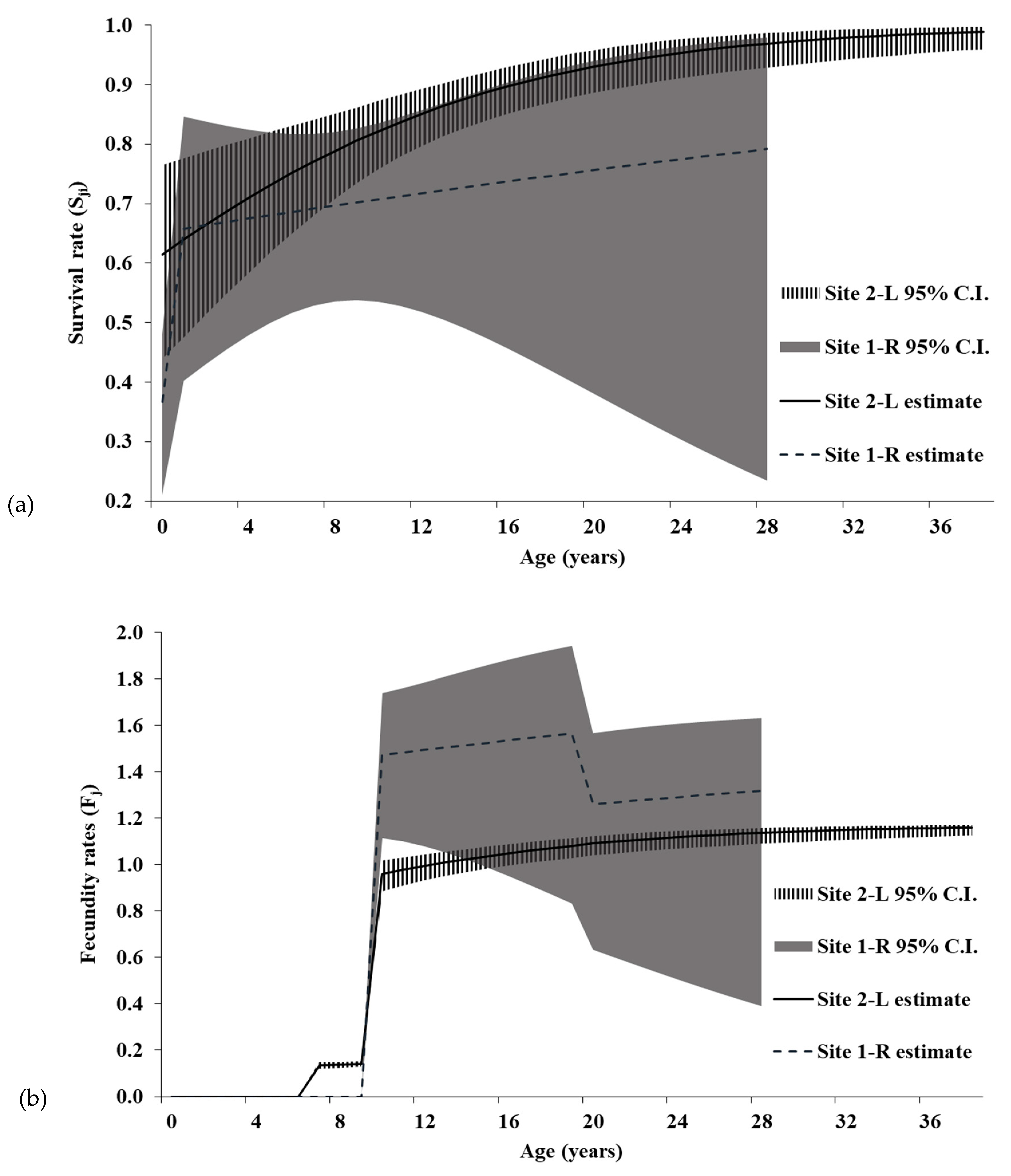
Our results indicate that age-specific survival rates for Illinois Spotted Turtles (Clemmys guttata) follow a similar ontogenetic trend and value as those documented for other freshwater turtle species [24], with survival sometimes reaching over 90% in adults [27,47]. Old adults have higher survival rates than young adults, similar to what is found in the Blanding’s Turtle (Emydoidea blandingii) [48]. Illinois populations show elastic prioritization of vital rates often seen in long-lived turtle species [24], using a bet-hedging life history strategy with adult survival having the largest proportional impact on population growth rate. Our study also indicates a demographic divergence between Illinois populations and suggests clinal variation in demographic rates when viewed in a larger geographic context. Though estimated population sizes have increased since 1988 [45], current projections from the Leslie matrices suggests both populations will likely begin to decline. Management to ensure high adult survival and conserve or expand existing habitat will likely be necessary.
A review of survivorship in 25 turtle species showed an average survival rate of 86.6%, with all but four species having >80% annual survival [49]. Illinois populations of C. guttata have comparable survival rates to turtles documented in the review [49]. Site 2-L bounds the estimate from an Ontario C. guttata population of 96.5% [15], suggesting adults in demographically healthy C. guttata populations should be above 90% annual survival. The juvenile C. guttata survival rate from the northern edge of the range was 81.6% [15], one of the highest reported for freshwater turtle species and comparable to the upper 95% C.I. estimates for Illinois populations. Furthermore, these estimated survival rates were within the range reported for other species. For instance, juvenile Emydoidea blandingii [32], Yellow Mud Turtles (Kinosternon flavescens) [50], Eastern Mud Turtles (K. subrubrum) [34], and Painted Turtles (Chrysemys picta) [9] all had survival estimates ranging from 64.0% to 80.6%.
Female age-specific fecundity results support findings from an Ontario study [30], which concluded C. guttata exemplifies the ‘terminal investment hypothesis’ of reproduction in which individuals with a low probability of surviving to future reproductive events increase their present reproductive investment [51]. Higher ASRO could represent a trade-off in resource allocation [52] whereby greater present maternal investment correlates with reduced future body condition, growth, and survival [53]. For instance, studies on C. guttata from South Carolina and Canada found larger clutch sizes correlated with both poor and good maternal body condition [30,54]. The Chicken Turtle (Deirochelys reticularia) exhibits an extreme version of the terminal investment life history strategy where females have high fertility (annual reproduction of large clutches), mature early (age 2–5 years), and have >30% mortality rates in response to extreme environmental stochasticity [
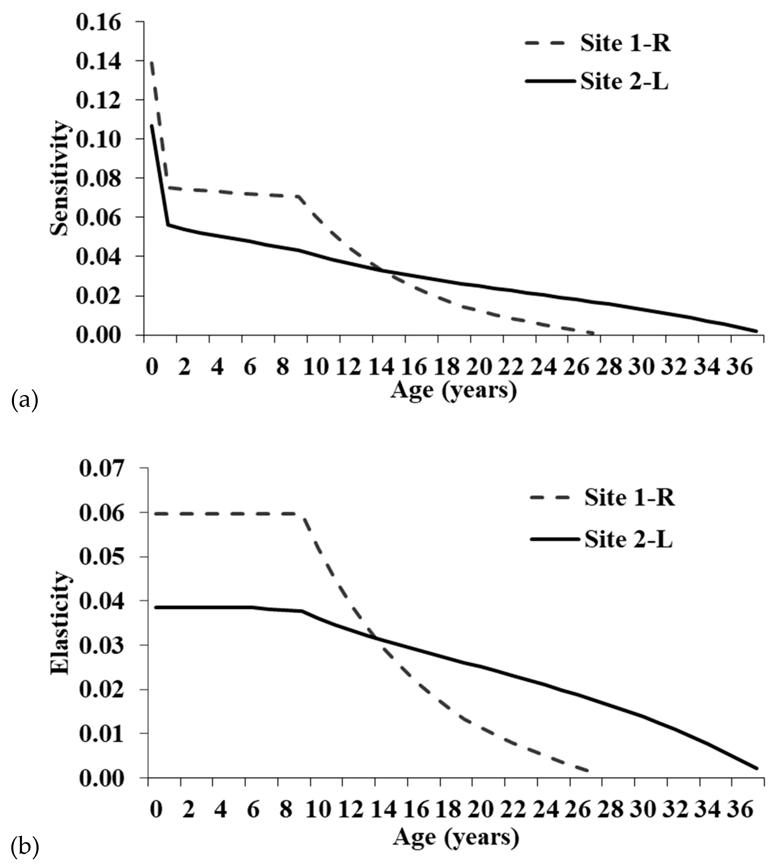
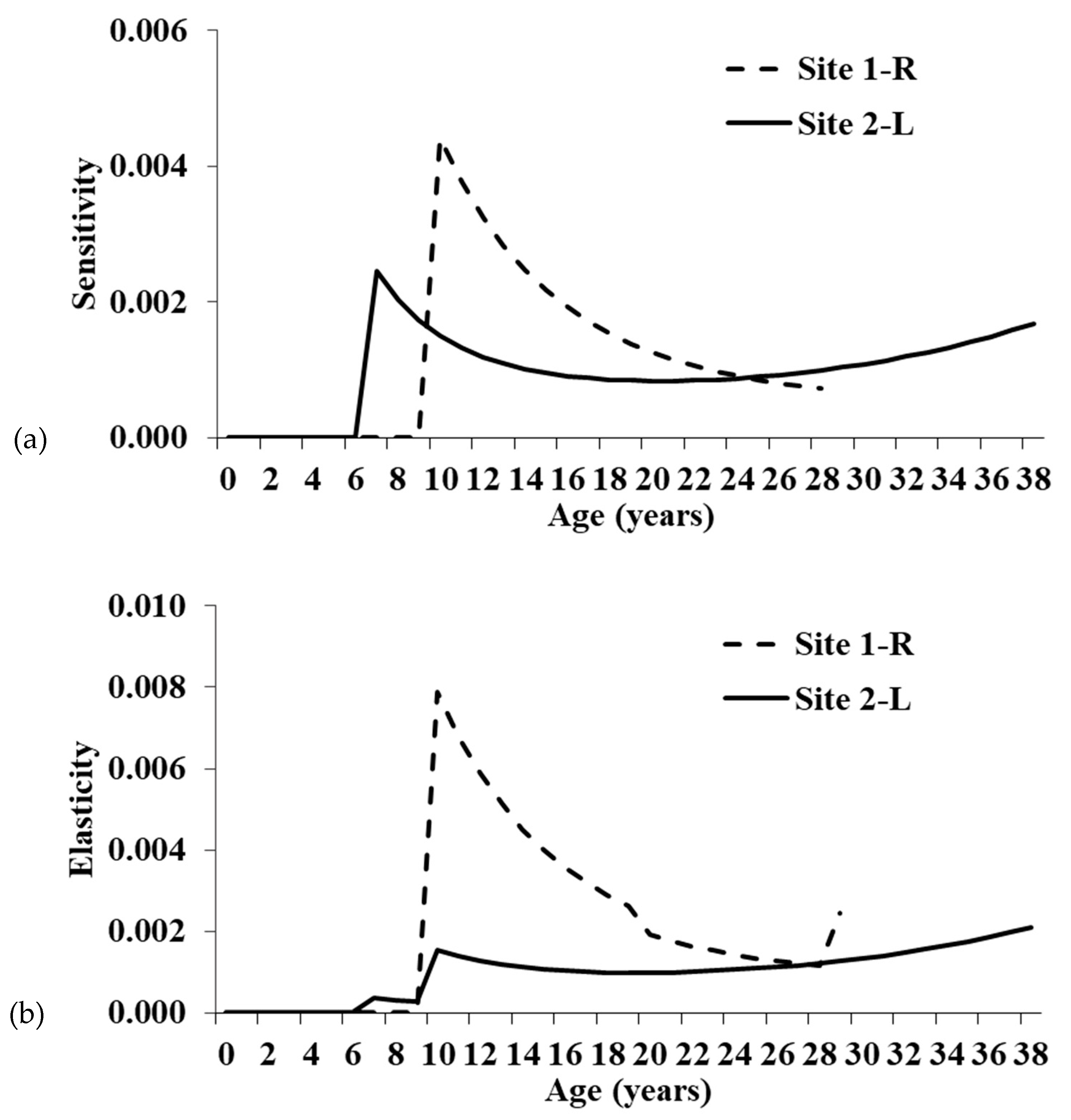
55]. Although individuals at Site 1-R have greater ASRO than at Site 2-L, all fecundity elements of the Leslie matrices have low sensitivities and elasticities, suggesting the increased clutch size has minimal ability to alter the population trajectory at Site 1-R (Figure 6).
While the single-year age classes with the greatest proportional influence on population growth were pre-reproductive survival, adult survival has the highest summed elasticity of the three main stage groups (hatchling, juvenile, and adult). Thus, conservation actions targeting adults will have the greatest proportional impact on the population growth rate. Focusing on the summed elasticities is preferable because management will typically impact a life history stage, not specific age classes [24]. Though adult elasticity is highest, juvenile survival also has moderate elasticity, particularly at Site 1-R.
The summed elasticities are comparable to those derived from a stage-based matrix for an Ontario population [15]. Elasticities for Site 2-L were very similar to the Ontario population, whereas elasticities were relatively higher for juveniles and lower for adults at Site 1-R. The increased elasticity for younger turtles at Site 1-R is likely related to the maximum age in the models and lower annual survival. The maximum age for Site 1-R was only 28 years, whereas Site 2-L was 38 years, and the Ontario study did not include a maximum age [15]. Having fewer individuals surviving to old age will increase the importance of younger turtles in maintaining the population and result in higher elasticity values. This is also noticeable when comparing the three adult stage categories for the Illinois populations. Mature adult elasticity is similar between sites, but the relatively high elasticity seen for old adults at Site 2-L is shifted to juveniles and young adults at Site 1-R. Clemmys guttata are estimated to live at least 60 and maybe even >100 years [37], so in areas where individuals attain higher maximum ages, mature adult survival elasticity should be higher. Elasticities for fecundity were also similar between the Illinois and Ontario populations.
Our results support previous studies that concluded C. guttata uses a bet-hedging life history strategy where higher adult survival and longevity compensate for lower juvenile survival and recruitment [15,37]. However, the bet hedging is not as extreme as seen in some other chelonian species. For instance, total adult elasticity typically increases with the amount of bet hedging [29], and a Snapping Turtle (Chelydra serpentina) population in Ontario had a total adult elasticity of ~87% [29]. At Site 1-R, longevity and adult survival elasticity were somewhat lower than Site 2-L. However, if mortality rates at Site 1-R are high due to anthropogenic disturbances, the juvenile elasticities may be elevated simply because the maximum age of adults is not as high as it would be in an undisturbed natural landscape. Thus, in an undisturbed population, adults would attain higher maximum ages and have higher summed elasticity.
Further examination of life-history traits can highlight interesting differences between C. guttata and other sympatric wetland turtle species. Clemmys guttata attains sexual maturity at a moderate age [49], has comparably high adult survivorship [27,56,57], low reproductive output [58,59], and moderate longevity [60]. Among animals with high adult survival rates, some species have multiple clutches per year and/or large clutch sizes, whereas others invest more heavily in one or a few offspring [61]. Some studies have found C. guttata have multiple clutches per year [62], though clutch size is relatively small compared to species such as C. serpentina or E. blandingii [63,64]. Thus, C. guttata may be investing slightly more in fewer offspring than sympatric wetland turtle species. This could account for pre-reproductive age-classes having the highest single elasticity values in our study.
Though many turtles rely on longevity and high adult survival as a life-history strategy, there are exceptions. For example, recent demographic studies on the genus Chelodina counter the assumed chelonian life-history strategies. The population growth rates of the Snake-necked Turtle (Chelodina rugosa) are fairly resistant to adult removal [65], whereas λ of the congeneric Eastern Long-necked Turtle (Chelodina longicollis) is most sensitive to adult survival but cannot exceed 1.0 without increased hatchling survival [66]. Moreover, while lengthy studies are resource-intensive, short-term evaluation may simply not consistently represent a population’s fundamental demographic behavior and lead to spurious conclusions [67]. As more long-term demographic analyses are produced for more species, we will improve our understanding of the variation in turtle life-history strategies.
Our results additionally show evidence of demographic divergence between the Illinois populations. First, the Illinois populations were not consistent with each other concerning the shape of the survival curves and their estimated magnitudes. More specifically, at Site 1-R, determining if and where an asymptote exists may only be resolved through continued monitoring to track older marked individuals. The 10-yr dataset of >100 individuals for Site 1-R may be insufficient to characterize the population despite its 21-yr span. More frequent surveys as were conducted at Site 2-L may be required to produce reliable estimates and mitigate the low certainty in Site 1-R survival rates. Alternatively, if the modeled variability in survival for adults is not exaggerated, the given estimates reveal a population vulnerable to the effects of demographic and environmental stochasticity, which can quickly lead to extirpation [68]. Selection may temper this risk for larger clutch sizes leading to higher ASRO at Site 1-R to compensate for lower or more variable adult survival than at Site 2-L. We speculate the demographic divergence between populations to be an adaptive response to human-induced rapid environmental change, which can lead to sudden increases in trait plasticity [69]. Previous research has demonstrated fast evolutionary responses with large populations or short generation times [70,71], but our results show a demographic response to recent habitat loss and fragmentation (~200 years or ~10 generations). Research at the northern range limit of C. guttata demonstrated substantial demographic variability could occur at more local scales between disparate habitat types [72], but we further demonstrate detectable demographic plasticity between conspecific populations located in similar and nearby sites. This variation is evidence of the demographic expression of genetic divergence between Illinois populations [39].
Our study also provides further support for clinal variation in demographic properties. In general, chelonian size and egg mass positively correlate with latitude [73,74], whereas clutch size decreases with latitude [75]. In the Wood Turtle (Glyptemys insculpta), life-history traits of body size and clutch size vary by latitude due to a combination of demographic and environmental factors [76]. Likewise, in C. picta, northern populations produce an average of 10.7 eggs per clutch as compared with 4.1 eggs per clutch in southern populations [77]. Life-history traits are thus known to vary, sometimes starkly, within species [78,79]. Similarly, C. guttata exhibits clinal variation in average clutch size across its broad range [80]. We documented average clutch size (eggs per reproductive female) in Illinois populations (41°N; Site 1-R = 4.35 ± 0.95, Site 2-L = 3.34 ± 0.91) as intermediate between Ontario (45°N; 5.3 ± 0.04) and Pennsylvania (40°N; 3.9 ± 0.01) but with greater variability [62]. Survival estimates for C. picta from Michigan show two-fold higher survival rates compared with estimates from South Carolina [9,81], and C. guttata appears to follow a similar trend with increasing juvenile survival with latitude.
The variation from our calculation of age-specific traits revealed trends between Illinois populations and between Illinois and Canadian C. guttata. First, G1-R (14.9 years) was roughly 65% of G2-L (22.8 years), indicating the mean age of reproduction is significantly younger for Site 1-R than Site 2-L individuals, likely due to lower adult survival rates [82]. Both Illinois populations had shorter generation times than the Ontario population (Table 2; Gont = 27.8 years), reinforcing the known positive correlation between G and latitude in ectotherms [83,84]. The most accurate estimate of maximum longevity (a) using the Litzgus [37] formulation for either site is obscured by the sensitivity of the equation to small changes in survival and the large C.I. for adult survival. At Site 2-L, for example, a difference in estimated survival of ~2.5% resulted in a 35-yr alteration between the PE and UCE estimates. However, a for female C. guttata was much lower in Illinois than in Canada even when using the larger UCE from Illinois for comparison. In C. guttata, the clinal trend may be further explained by the short active season of northern turtle species, which experience lower annual metabolic activity [31] due to an overwintering period of six months per year [85]. The restrictive environmental conditions in Canada are consequently reflected in C. guttata life history and include higher survival by stage [15], later attainment of sexual maturity [37], and greater estimated longevity [37]. It follows that G, as a measure of the average age of mothers at childbirth [3], would be larger at higher latitudes. However, larger estimates of G correspond to slower recovery from overexploitation or other high mortality events [27,65], which may pose a threat to Canadian C. guttata.
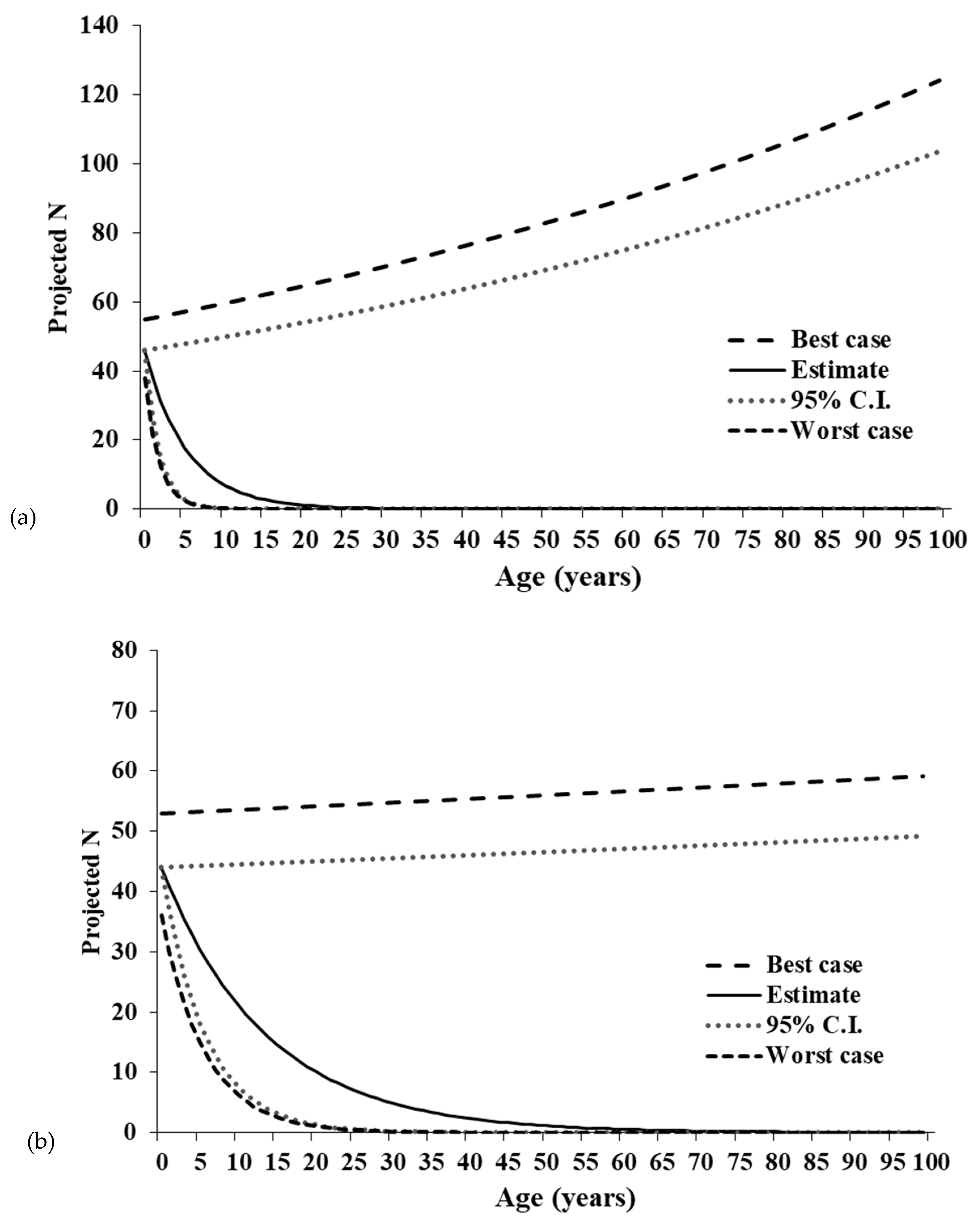
Moreover, the related terms of R0 and λ suggest a greater divergence in deterministic trends between Illinois and Canada. Our results show a demographically driven decline in the Site 1-R population, made obvious by population projections. Given deterministic conditions, the estimated 95% LCE, and worst-case scenarios closely track one another to show an estimated reduction to one female individual within 17 years in the Site 1-R population. The projections showing rapid population growth for the Site 1-R UCE and best-case scenarios are thus likely exaggerated and unreliable. The Site 2-L population exhibits only minor growth even in the deterministic best case and UCE scenarios, so it is likely that neither population is demographically viable under stochastic conditions. In contrast, the Ontario population exhibits a positive λ and R0 an order of magnitude above Illinois estimates.
The negative population growth rates derived from the Leslie matrices were surprising because population size estimates from a POPAN model previously indicated the populations were experiencing stable to increasing abundance since 1988 [45]. We posit three related causes for the discrepancy in our findings. First, our initial abundance estimates included males, while our matrix models were female-only. We assumed the single-sex model was representative of the entire population, but it is possible male dynamics differ from and obscure trends in female dynamics [86]. We do not consider this problematic as C. guttata reproduces sexually, and female abundance is a limiting factor for population growth. Second, our previous estimates of λ were based on a small sample size of capture data (n1-R = 6, n2-L = 11) and may be elevated as a result of population momentum [82]. In other words, the populations were sampled while experiencing short-term, transient dynamics, not representative of the general trend [87]. This explanation only reemphasizes the necessity of long-term datasets for long-lived species [88]. Finally, our calculation of 
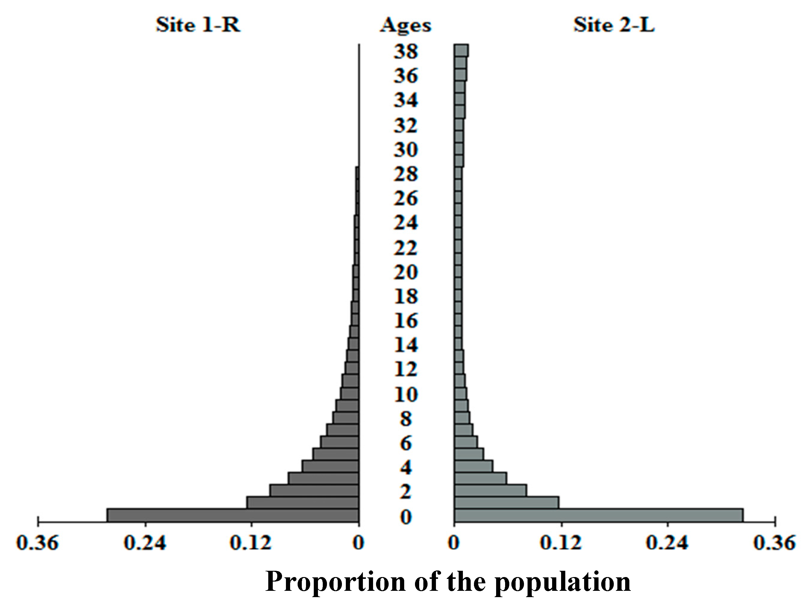
λ assumes the populations have achieved a stable age distribution. However, the damping ratio (ρ), a measure of the rapidity of convergence on the stable age distribution (n; Figure 4), is low for each population (ρ < 1.1). While low ρ is expected for a long-lived species [89], it also suggests C. guttata recovers slowly from alterations to the age distribution. Illinois populations may be experiencing short-term growth over the length of the study (equal to 1–2 generation times) while equilibrating toward n, but this growth is unlikely to be sustained.
The intraspecific variation between our highly proximate populations of C. guttata suggests demographic plasticity is an adaptive response to site-specific challenges. However, we add the caveat that elasticity matrices derived from inaccurate estimates of vital rates over the short term [11] or from changes in vital rates over time [90] could lead to misprioritization of age classes to target for conservation. In our analysis, the incorrect ranking could be due to two main factors. First, ASRO based on size is likely more appropriate than age-based ASRO as size correlates more strongly with the onset of sexual maturity and clutch size in turtles [
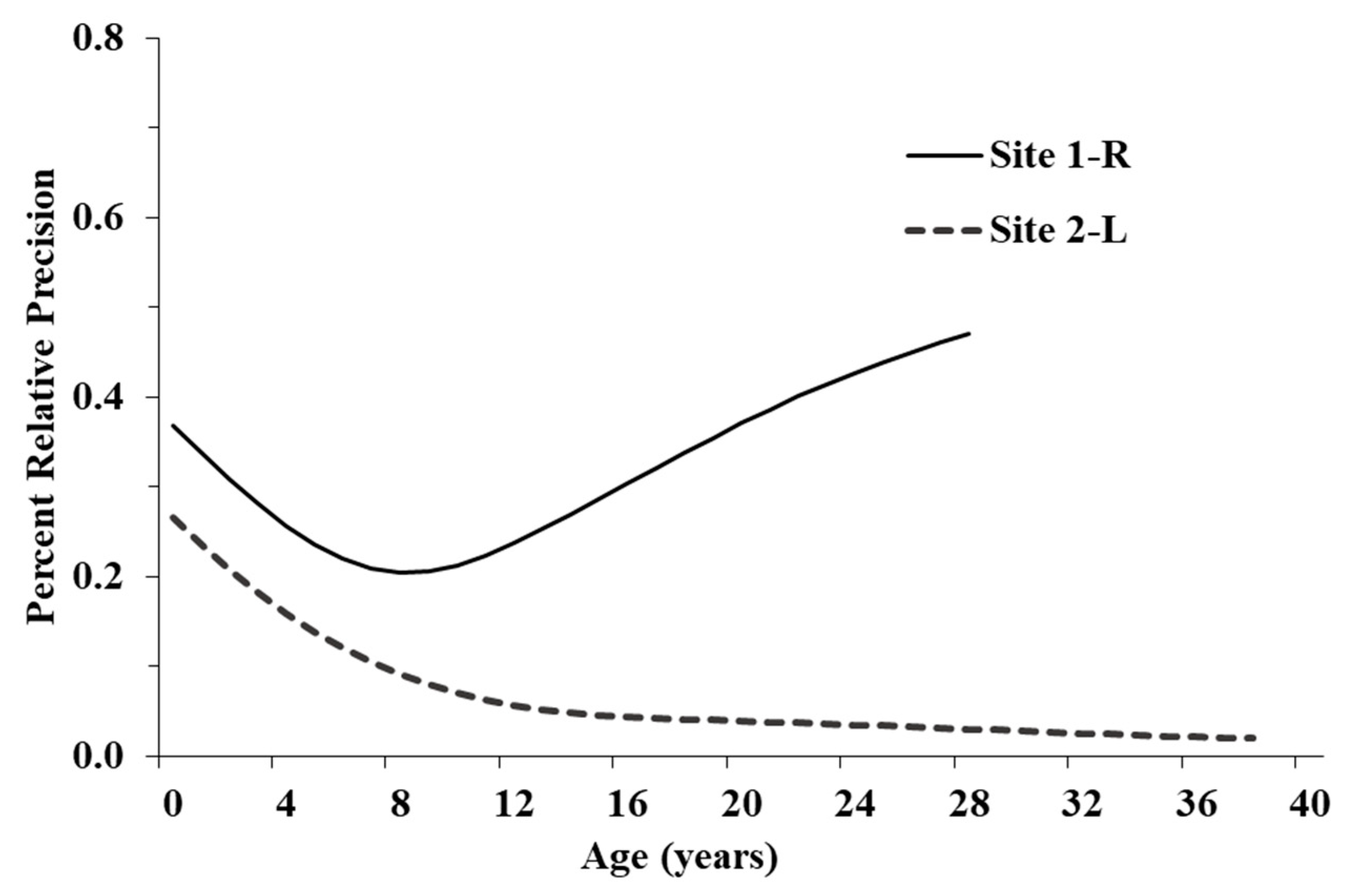
91]. We recommend restructuring fecundity based on size classes and using regression analysis to relate size classes with age classes. Second, the large confidence intervals and high PRP (Figure 4) for younger age classes, most noticeably at Site 1-R, suggest future research should focus on eggs, hatchlings, and juveniles [37]. Major changes between current and future vital rates will likely be attributable to habitat improvements and can be recalculated to determine the efficacy of our recommendations to promote population growth. Moreover, it would be interesting to see if both populations respond to the same management actions to the same degree.
Our study indicates management actions targeting adult survival will have the greatest proportional impact on population growth rate. The other long-term study on C. guttata in Ontario also found adult survival to be important [15], so this is likely the case throughout the species range. In Illinois, adult survival likely needs to be increased at Site 1-R and at least maintained at Site 2-L. Preventing adult removal or mortality from collecting and roads will be beneficial. The variation in vital rates and relatively higher elasticity of juveniles at Site 1-R indicates a demographic divergence between populations. Thus, prioritization of vital rates can vary even over a small geographic area, so juvenile and age 0-1 survival cannot be totally ignored. In some cases, mesopredators can eliminate entire cohorts of turtles in isolated populations [92]. If adult survival is known to be high and a population is still declining, management targeting juvenile or egg and hatchling survival could still be necessary. Caging nests and trapping mesopredators are effective methods to reduce predation of nests and juveniles [93,94]. Captive rearing and head-starting are more manipulative methods for recovering small, highly impacted populations [24]. Though adults are more resilient to predation attempts than juveniles [95] and often only lose limbs or accrue shell scours (pers. obs.), they may also benefit from fewer interactions with predators [96,97] or from allocating fewer resources to recovering from predator-induced injury [98]. Thus, the removal of mesopredators would likely benefit all stages simultaneously. Increasing high-quality nesting habitat would also increase the number of surviving eggs and reduce predation risks to adult females [99,100].
Clemmys guttata inhabits a variety of shallow aquatic habitats in variable climates throughout the eastern United States, including swamps, bogs, fens, ephemeral pools, cattail marshes, sedge meadows, and drainage ditches [60,101]. Thus, habitat management aimed at increasing survival rate or population size should consider habitat characteristics and vegetation at a site-specific or regional scale. Our trapping indicates Illinois populations are limited to core habitat areas featuring necessary components, such as permanent shallow-water wetlands with overwintering burrows. These areas need to be carefully maintained at a minimum, and additional habitat restoration may be beneficial. For instance, at Site 2-L, we captured new individuals in a habitat that was restored in the late 1990s. However, at Site 1-R, changes in plant community composition have occurred in core habitats, with a pronounced expansion of Typha spp. at the expense of more open Carex wetlands. Expanding the amount of suitable habitat through restoration and management is particularly needed at Site 1-R to increase adult survival rates. The change in vegetation has also caused a drawdown of available standing water, perhaps contributing to lower survival rates and longevity. Given that wetlands inhabited by C. guttata are already shallow, any additional lowering of water levels would greatly hinder conservation efforts. Controlled burns during the non-active season of C. guttata can be used to help reverse unwanted successional trends in vegetation [102].

Author Contributions

Conceptualization, C.Y.F., D.M., and M.J.D.; data curation, C.Y.F., J.P.R., D.M., and M.J.D.; formal analysis, C.Y.F.; funding acquisition, C.Y.F., D.M., and M.J.D.; investigation, C.Y.F., J.P.R., D.M., and M.J.D.; methodology, C.Y.F., J.P.R., D.M., and M.J.D.; project administration, M.J.D.; resources, D.M. and M.J.D.; software, C.Y.F., J.P.R., and M.J.D.; supervision, C.Y.F. and M.J.D.; validation, C.Y.F., J.P.R., and M.J.D.; visualization, C.Y.F., J.P.R., D.M., and M.J.D.; writing – original draft, C.Y.F.; writing – review and editing, J.P.R., D.M., and M.J.D.

Funding

This research was funded by the Illinois State Toll Highway Authority, the Illinois Department of Natural Resources, the University of Illinois at Urbana-Champaign, and the local Forest Preserve District. All work was covered under appropriate permits with the Illinois Department of Natural Resources T&E permit and in accordance with approved IACUC Protocol #14000 with the University of Illinois.

Acknowledgments

Our special thanks to Whitney J.B. Anthonysamy and Tom Wilson Jr. for their dedication and data. We thank Christopher A. Phillips and Cory Suski for helpful comments on early drafts. We thank field assistants Kelsey Low, Ellie Moen, and Claire Butkus for their work on the study. We also thank Charles Warwick for providing technical editorial comments on the draft manuscript and Jennifer Mui for assistance with graphics.

Conflicts of Interest

The authors declare no conflict of interest. The funders had no role in the design of the study; in the collection, analyses, or interpretation of data; in the writing of the manuscript; or in the decision to publish the results.

Appendix A

Table A1. Leslie matrix elements for Illinois populations of Clemmys guttata in which j = Age in years, i = j + 1, Sji = survival from age j to i, and Fj = fecundity of age j. All non-listed elements are equal to 0.
Site 1-RSite 2-L
jSjiFjjSjiFj
00.356 (0.210, 0.467)000.336 (0.240, 0.418)0
10.658 (0.402, 0.846)010.640 (0.476, 0.776)0
20.664 (0.429, 0.838)020.664 (0.512, 0.788)0
30.669 (0.455, 0.831)030.687 (0.548, 0.799)0
40.675 (0.479, 0.824)040.709 (0.584, 0.809)0
50.680 (0.499, 0.819)050.731 (0.618, 0.820)0
60.686 (0.516, 0.817)060.751 (0.650, 0.831)0
70.691 (0.528, 0.817)070.770 (0.680, 0.841)0.136 (0.120, 0.148)
80.697 (0.536, 0.820)080.789 (0.708, 0.851)0.139 (0.125, 0.150)
90.702 (0.538, 0.826)090.806 (0.734, 0.862)0.142 (0.130, 0.152)
100.707 (0.535, 0.835)1.473 (1.115, 1.740)100.822 (0.757, 0.872)0.961 (0.886, 1.020)
110.712 (0.528, 0.845)1.484 (1.100, 1.761)110.837 (0.778, 0.882)0.979 (0.910, 1.032)
120.717 (0.518, 0.857)1.495 (1.079, 1.785)120.851 (0.797, 0.892)0.995 (0.932, 1.044)
130.722 (0.505, 0.869)1.505 (1.053, 1.810)130.864 (0.813, 0.902)1.010 (0.951, 1.055)
140.727 (0.490, 0.881)1.516 (1.022, 1.835)140.876 (0.827, 0.912)1.024 (0.968, 1.067)
150.732 (0.474, 0.893)1.526 (0.987, 1.860)150.887 (0.840, 0.921)1.037 (0.983, 1.077)
160.737 (0.456, 0.904)1.536 (0.951, 1.883)160.897 (0.851, 0.930)1.049 (0.996, 1.088)
170.742 (0.438, 0.914)1.546 (0.912, 1.904)170.906 (0.861, 0.938)1.060 (1.008, 1.097)
180.747 (0.419, 0.924)1.556 (0.873, 1.924)180.915 (0.870, 0.945)1.070 (1.018, 1.106)
190.752 (0.400, 0.932)1.566 (0.832, 1.942)190.923 (0.879, 0.952)1.080 (1.028, 1.114)
200.756 (0.380, 0.940)1.261 (0.633, 1.567)200.930 (0.886, 0.958)1.092 (1.040, 1.125)
210.761 (0.361, 0.947)1.268 (0.601, 1.579)210.937 (0.893, 0.963)1.100 (1.048, 1.131)
220.766 (0.341, 0.954)1.276 (0.569, 1.589)220.943 (0.899, 0.968)1.107 (1.055, 1.137)
230.770 (0.322, 0.959)1.283 (0.537, 1.599)230.948 (0.905, 0.972)1.113 (1.062, 1.141)
240.774 (0.304, 0.964)1.291 (0.506, 1.607)240.953 (0.910, 0.976)1.119 (1.069, 1.146)
250.779 (0.285, 0.969)1.298 (0.476, 1.615)250.958 (0.915, 0.979)1.124 (1.075, 1.150)
260.783 (0.268, 0.973)1.305 (0.446, 1.621)260.962 (0.920, 0.982)1.129 (1.080, 1.153)
270.787 (0.251, 0.976)1.312 (0.418, 1.627)270.966 (0.925, 0.985)1.133 (1.085, 1.156)
2801.319 (0.390, 1.632)280.969 (0.929, 0.987)1.137 (1.090, 1.158)
290.972 (0.933, 0.989)1.141 (1.095, 1.160)
300.975 (0.936, 0.990)1.144 (1.099, 1.162)
310.977 (0.940, 0.992)1.147 (1.103, 1.164)
320.979 (0.943, 0.993)1.150 (1.107, 1.165)
330.981 (0.946, 0.994)1.152 (1.111, 1.167)
340.983 (0.949, 0.995)1.154 (1.114, 1.168)
350.985 (0.952, 0.995)1.156 (1.118, 1.168)
360.986 (0.955, 0.996)1.158 (1.121, 1.169)
370.988 (0.957, 0.997)1.160 (1.124, 1.170)
3801.161 (1.126, 1.170)

Appendix B

Table A2. Sensitivity matrix elements for Illinois populations of Clemmys guttata in which j = Age in years, i = j + 1, Sji = sensitivity of survival from age j to i, and Fj = sensitivity of fecundity of age j. All non-listed elements are equal to 0. Values in parentheses are sensitivities calculated from Leslie matrices of the LCE and UCE.
Site 1-RSite 2-L
jSjiFjjSjiFj
00.139 (0.188, 0.127)000.107 (0.115, 0.110)0
10.075 (0.098, 0.070)010.056 (0.058, 0.059)0
20.074 (0.092, 0.071)020.054 (0.054, 0.058)0
30.074 (0.087, 0.072)030.052 (0.050, 0.057)0
40.073 (0.083, 0.072)040.051 (0.047, 0.057)0
50.073 (0.079, 0.073)050.049 (0.045, 0.056)0
60.072 (0.077, 0.073)060.048 (0.043, 0.055)0
70.071 (0.075, 0.073)070.046 (0.041, 0.054)0.002 (0.001, 0.005)
80.071 (0.074, 0.073)080.045 (0.039, 0.052)0.002 (0.001, 0.004)
90.070 (0.074, 0.072)090.043 (0.037, 0.051)0.002 (0.001, 0.004)
100.061 (0.062, 0.062)0.004 (0.006, 0.005)100.041 (0.036, 0.047)0.001 (0.001, 0.003)
110.052 (0.051, 0.053)0.004 (0.005, 0.004)110.039 (0.034, 0.043)0.001 (0.000, 0.003)
120.045 (0.041, 0.046)0.003 (0.005, 0.003)120.037 (0.033, 0.040)0.001 (0.000, 0.002)
130.039 (0.033, 0.040)0.003 (0.005, 0.003)130.035 (0.032, 0.037)0.001 (0.000, 0.002)
140.034 (0.025, 0.034)0.002 (0.004, 0.002)140.033 (0.031, 0.034)0.001 (0.000, 0.002)
150.029 (0.019, 0.029)0.002 (0.004, 0.002)150.032 (0.030, 0.032)0.001 (0.000, 0.002)
160.025 (0.014, 0.025)0.002 (0.003, 0.002)160.030 (0.029, 0.029)0.001 (0.000, 0.002)
170.021 (0.009, 0.022)0.002 (0.002, 0.002)170.029 (0.028, 0.027)0.001 (0.000, 0.002)
180.018 (0.006, 0.018)0.002 (0.002, 0.001)180.027 (0.027, 0.026)0.001 (0.000, 0.001)
190.015 (0.004, 0.015)0.001 (0.001, 0.001)190.026 (0.027, 0.024)0.001 (0.000, 0.001)
200.012 (0.002, 0.013)0.001 (0.001, 0.001)200.025 (0.026, 0.022)0.001 (0.000, 0.001)
210.010 (0.001, 0.011)0.001 (0.001, 0.001)210.024 (0.025, 0.021)0.001 (0.000, 0.001)
220.009 (0.001, 0.009)0.001 (0.000, 0.001)220.023 (0.024, 0.019)0.001 (0.000, 0.001)
230.007 (0.000, 0.008)0.001 (0.000, 0.001)230.022 (0.024, 0.018)0.001 (0.001, 0.001)
240.005 (0.000, 0.006)0.001 (0.000, 0.001)240.020 (0.023, 0.016)0.001 (0.001, 0.001)
250.004 (0.000, 0.004)0.001 (0.000, 0.001)250.019 (0.022, 0.015)0.001 (0.001, 0.001)
260.003 (0.000, 0.003)0.001 (0.000, 0.001)260.018 (0.021, 0.014)0.001 (0.001, 0.001)
270.001 (0.000, 0.001)0.001 (0.000, 0.001)270.017 (0.020, 0.013)0.001 (0.001, 0.001)
2800.001 (0.000, 0.001)280.016 (0.019, 0.011)0.001 (0.001, 0.001)
290.014 (0.018, 0.010)0.001 (0.001, 0.001)
300.013 (0.017, 0.009)0.001 (0.001, 0.001)
310.012 (0.015, 0.008)0.001 (0.001, 0.001)
320.010 (0.014, 0.007)0.001 (0.001, 0.001)
330.009 (0.012, 0.006)0.001 (0.001, 0.001)
340.007 (0.010, 0.004)0.001 (0.002, 0.001)
350.006 (0.008, 0.003)0.001 (0.002, 0.001)
360.004 (0.006, 0.002)0.001 (0.002, 0.001)
370.002 (0.003, 0.001)0.002 (0.002, 0.001)
3800.002 (0.003, 0.001)

Appendix C

Table A3. Elasticity matrix elements for Illinois populations of Clemmys guttata in which j = Age in years, i = j + 1, Sji = elasticity of survival from age j to i, and Fj = elasticity of fecundity of age j. All non-listed elements are equal to 0. Values in parentheses are elasticities calculated from Leslie matrices of the LCE and UCE.
Site 1-RSite 2-L
jSjiFjjSjiFj
00.060 (0.069, 0.059)0 (0, 0)00.039 (0.033, 0.046)0
10.060 (0.069, 0.059)0 (0, 0)10.039 (0.033, 0.046)0
20.060 (0.069, 0.059)0 (0, 0)20.039 (0.033, 0.046)0
30.060 (0.069, 0.059)0 (0, 0)30.039 (0.033, 0.046)0
40.060 (0.069, 0.059)0 (0, 0)40.039 (0.033, 0.046)0
50.060 (0.069, 0.059)0 (0, 0)50.039 (0.033, 0.046)0
60.060 (0.069, 0.059)0 (0, 0)60.039 (0.033, 0.046)0
70.060 (0.069, 0.059)0 (0, 0)70.038 (0.033, 0.045)0.000 (0.000, 0.001)
80.060 (0.069, 0.059)0 (0, 0)80.038 (0.033, 0.044)0.000 (0.000, 0.001)
90.060 (0.069, 0.059)0 (0, 0)90.038 (0.033, 0.044)0.000 (0.000, 0.001)
100.052 (0.058, 0.051)0.008 (0.011, 0.008)100.036 (0.032, 0.041)0.002 (0.001, 0.003)
110.045 (0.047, 0.045)0.007 (0.011, 0.007)110.035 (0.032, 0.038)0.001 (0.000, 0.003)
120.039 (0.038, 0.039)0.006 (0.010, 0.006)120.033 (0.031, 0.035)0.001 (0.000, 0.003)
130.034 (0.029, 0.034)0.005 (0.009, 0.005)130.032 (0.031, 0.033)0.001 (0.000, 0.002)
140.030 (0.022, 0.030)0.005 (0.007, 0.004)140.031 (0.030, 0.031)0.001 (0.000, 0.002)
150.026 (0.016, 0.026)0.004 (0.006, 0.004)150.030 (0.030, 0.029)0.001 (0.000, 0.002)
160.022 (0.011, 0.023)0.004 (0.005, 0.003)160.029 (0.029, 0.027)0.001 (0.000, 0.002)
170.019 (0.007, 0.020)0.003 (0.004, 0.003)170.028 (0.029, 0.026)0.001 (0.000, 0.002)
180.016 (0.004, 0.017)0.003 (0.003, 0.003)180.027 (0.028, 0.024)0.001 (0.000, 0.002)
190.013 (0.002, 0.014)0.003 (0.002, 0.003)190.026 (0.028, 0.023)0.001 (0.001, 0.001)
200.011 (0.001, 0.012)0.002 (0.001, 0.002)200.025 (0.027, 0.021)0.001 (0.001, 0.001)
210.001 (0.001, 0.011)0.002 (0.001, 0.002)210.024 (0.027, 0.020)0.001 (0.001, 0.001)
220.008 (0.000, 0.009)0.002 (0.000, 0.002)220.023 (0.026, 0.018)0.001 (0.001, 0.001)
230.006 (0.000, 0.007)0.002 (0.000, 0.002)230.022 (0.026, 0.017)0.001 (0.001, 0.001)
240.005 (0.000, 0.006)0.001 (0.000, 0.002)240.021 (0.025, 0.016)0.001 (0.001, 0.001)
250.004 (0.000, 0.004)0.001 (0.000, 0.001)250.020 (0.024, 0.015)0.001 (0.001, 0.001)
260.002 (0.000, 0.003)0.001 (0.000, 0.001)260.019 (0.023, 0.013)0.001 (0.001, 0.001)
270.001 (0.000, 0.001)0.001 (0.000, 0.001)270.018 (0.022, 0.012)0.001 (0.001, 0.001)
2800.001 (0.000, 0.001)280.016 (0.021, 0.011)0.001 (0.001, 0.001)
290.015 (0.020, 0.010)0.001 (0.001, 0.001)
300.014 (0.019, 0.009)0.001 (0.001, 0.001)
310.012 (0.017, 0.008)0.001 (0.001, 0.001)
320.011 (0.016, 0.007)0.001 (0.002, 0.001)
330.009 (0.014, 0.005)0.002 (0.002, 0.001)
340.008 (0.012, 0.004)0.002 (0.002, 0.001)
350.006 (0.009, 0.003)0.002 (0.002, 0.001)
360.004 (0.007, 0.002)0.002 (0.003, 0.001)
370.002 (0.004, 0.001)0.002 (0.003, 0.001)
3800.002 (0.004, 0.001)

References

  1. Dunham, A.E.; Miles, D.B. Patterns of covariation in life history traits of squamate reptiles: The effects of size and phylogeny reconsidered. Am. Nat. 1985, 126, 231–257. [Google Scholar] [CrossRef]
  2. Roff, D.A. Life History Evolution; Sinauer Associates: Sunderland, MA, USA, 2002; p. 527. [Google Scholar]
  3. Stearns, S.C. The Evolution of Life Histories; Oxford University Press: Oxford, UK, 1992; p. 264. [Google Scholar]
  4. Chaloupka, M.; Limpus, C. Estimates of sex-and age-class-specific survival probabilities for a southern Great Barrier Reef green sea turtle population. Mar. Biol. 2005, 146, 1251–1261. [Google Scholar] [CrossRef]
  5. Musolin, D.L. Insects in a warmer world: Ecological, physiological and life-history responses of true bugs (Heteroptera) to climate change. Glob. Chang. Biol. 2007, 13, 1565–1585. [Google Scholar] [CrossRef]
  6. Jonsson, A.; Ebenman, B. Are certain life histories particularly prone to local extinction? J. Theor. Biol. 2001, 209, 455–463. [Google Scholar] [CrossRef]
  7. Traill, L.W.; Brook, B.W.; Frankham, R.R.; Bradshaw, C.J.A. Pragmatic population viability targets in a rapidly changing world. Biol. Conserv. 2010, 143, 28–34. [Google Scholar] [CrossRef]
  8. Pearson, R.G.; Stanton, J.C.; Shoemaker, K.T.; Aiello-Lammens, M.E.; Ersts, P.J.; Horning, N.; Fordham, D.A.; Raxworthy, C.J.; Ryu, H.Y.; McNees, J.; et al. Life history and spatial traits predict extinction risk due to climate change. Nat. Clim. Chang. 2014, 4, 217–221. [Google Scholar] [CrossRef]
  9. Wilbur, H.M. The evolutionary and mathematical demography of the turtle Chrysemys picta. Ecology 1975, 56, 64–77. [Google Scholar] [CrossRef]
  10. Tuljapurkar, S.D.; Orzack, S.H. Population dynamics in variable environments I. Long-run growth rates and extinction. Theor. Popul. Biol. 1980, 18, 314–342. [Google Scholar] [CrossRef]
  11. Mills, L.S.; Lindberg, M.S. Sensitivity analysis to evaluate the consequences of conservation actions. In Population Viability Analysis; Beissinger, S.R., McCullough, D.R., Eds.; University of Chicago Press: Chicago, IL, USA, 2002; pp. 338–366. [Google Scholar]
  12. Auffarth, J.; Krug, A.; Pröehl, H.; Jehle, R. A genetically-informed population viability analysis reveals conservation priorities for an isolated population of Hyla arborea. Salamandra 2017, 53, 171–182. [Google Scholar]
  13. Hagen, C.A.; Sandercock, B.K.; Pitman, J.C.; Robel, R.J.; Applegate, R.D. Spatial variation in lesser prairie-chicken demography: A sensitivity analysis of population dynamics and management alternatives. J. Wildl. Manag. 2009, 73, 1325–1332. [Google Scholar] [CrossRef]
  14. Fujiwara, M.; Caswell, H. Demography of the endangered North Atlantic right whale. Nature 2001, 414, 537–541. [Google Scholar] [CrossRef] [PubMed]
  15. Enneson, J.J.; Litzgus, J.D. Using long-term data and a stage-classified matrix to assess conservation strategies for an endangered turtle (Clemmys guttata). Biol. Conserv. 2008, 141, 1560–1568. [Google Scholar] [CrossRef]
  16. Caswell, H. Matrix Population Models: Construction, Analysis, and Interpretation., 2nd ed.; Sinauer Associates Inc.: Sunderland, MA, USA, 2001; p. 722. [Google Scholar]
  17. Mogollones, S.C.; Rodríguez, D.J.; Hernández, O.; Barreto, G.R. A demographic study of the arrau turtle (Podocnemis expansa) in the Middle Orinoco River, Venezuela. Chelonian Conserv. Biol. 2010, 9, 79–89. [Google Scholar] [CrossRef]
  18. Zuidema, P.A.; Franco, M. Integrating vital rate variability into perturbation analysis: An evaluation for matrix population models of six plant species. J. Ecol. 2001, 89, 995–1005. [Google Scholar] [CrossRef]
  19. Sæther, B.-E.; Bakke, Ø. Avian life history variation and contribution of demographic traits to the population growth rate. Ecology 2000, 81, 642–653. [Google Scholar] [CrossRef]
  20. Akçakaya, H.R.; Radeloff, V.C.; Mladenoff, D.J.; He, H.S. Integrating landscape and metapopulation modeling approaches: Viability of the sharp-tailed grouse in a dynamic landscape. Conserv. Biol. 2004, 18, 526–537. [Google Scholar] [CrossRef]
  21. Berglind, S.Å. Population Dynamics and Conservation of the Sand Lizard (Lacerta agilis) on the Edge of its Range; Uppsala University: Uppsala, Sweden, 2005. [Google Scholar]
  22. Riedle, J.D. Demography of an urban population of ring-necked snakes (Diadophis punctatus) in Missouri. Herpetol. Conserv. Biol. 2014, 9, 278–284. [Google Scholar]
  23. Tinkle, D.W.; Congdon, J.D.; Rosen, P.C. Nesting frequency and success: Implications for the demography of painted turtles. Ecology 1981, 62, 1426–1432. [Google Scholar] [CrossRef]
  24. Heppell, S.S. Application of life-history theory and population model analysis to turtle conservation. Copeia 1998, 1998, 367–375. [Google Scholar] [CrossRef]
  25. Lovich, J.E.; Ennen, J.R. A quantitative analysis of the state of knowledge of turtles of the United States and Canada. Amphibia-Reptilia 2013, 34, 11–23. [Google Scholar] [CrossRef]
  26. Rhodin, A.G.; Stanford, C.B.; Van Dijk, P.P.; Eisemberg, C.; Luiselli, L.; Mittermeier, R.A.; Hudson, R.; Horne, B.D.; Goode, E.V.; Kuchling, G.; et al. Global conservation status of turtles and tortoises (Order Testudines). Chelonian Conserv. Biol. 2018, 17, 135–161. [Google Scholar] [CrossRef]
  27. Congdon, J.D.; Dunham, A.E.; van Loben Sels, R.C. Demographics of common snapping turtles (Chelydra serpentina): Implications for conservation and management of long-lived organisms. Am. Zool. 1994, 34, 397–408. [Google Scholar] [CrossRef]
  28. Janzen, F.J.; Tucker, J.K.; Paukstis, G.L. Experimental analysis of an early life-history stage: Selection on size of hatchling turtles. Ecology 2000, 81, 2290–2304. [Google Scholar] [CrossRef]
  29. Cunnington, D.C.; Brooks, R.J. Bet-hedging theory and eigenelasticity: A comparison of the life histories of loggerhead sea turtles (Caretta caretta) and snapping turtles (Chelydra serpentina). Can. J. Zool. 1996, 74, 291–296. [Google Scholar] [CrossRef]
  30. Litzgus, J.D.; Bolton, F.; Schulte-Hostedde, A.I. Reproductive output depends on body condition in spotted turtles (Clemmys guttata). Copeia 2008, 2008, 86–92. [Google Scholar] [CrossRef]
  31. Gibbons, J.W. Why do turtles live so long? Bioscience 1987, 37, 262–269. [Google Scholar] [CrossRef]
  32. Congdon, J.D.; Dunham, A.E.; van Loben Sels, R.C. Delayed sexual maturity and demographics of Blanding’s Turtles (Emydoidea blandingii): Implications for conservation and management of long-lived organisms. Conserv. Biol. 1993, 7, 826–833. [Google Scholar] [CrossRef]
  33. Johnson, K.A. The decline of the spotted turtle, Clemmys guttata, in northeastern Illinois. Bull. Chic. Herpetol. Soc. 1983, 18, 37–41. [Google Scholar]
  34. Frazer, N.B.; Gibbons, J.W.; Greene, J.L. Life history and demography of the common mud turtle Kinosternon subrubrum in South Carolina, USA. Ecology 1991, 72, 2218–2231. [Google Scholar] [CrossRef]
  35. Ernst, C.H.; Barbour, R.W. Turtles of the World; Smithsonian Institution: Washington, DC, USA, 1989; p. 313. [Google Scholar]
  36. COSEWIC. COSEWIC Assessment and Update Status Report on the Spotted Turtle Clemmys guttata in Canada; Committee on the Status of Endangered Wildlife in Canada: Ottawa, ON, Canada, 2004; p. 27. [Google Scholar]
  37. Litzgus, J.D. Sex differences in longevity in the spotted turtle (Clemmys guttata). Copeia 2006, 2006, 281–288. [Google Scholar] [CrossRef]
  38. Lindenmayer, D.; Scheele, B. Do not publish. Science 2017, 356, 800–801. [Google Scholar] [CrossRef] [PubMed]
  39. Anthonysamy, W.J.B.; Dreslik, M.J.; Douglas, M.R.; Thompson, D.; Klut, G.M.; Kuhns, A.R.; Mauger, D.; Kirk, D.; Glowacki, G.A.; Douglas, M.E.; et al. Population genetic evaluations within a co-distributed taxonomic group: A multi-species approach to conservation planning. Anim. Conserv. 2017, 21, 137–147. [Google Scholar] [CrossRef]
  40. Cagle, F.R. A system of marking turtles for future identification. Copeia 1939, 1939, 170–173. [Google Scholar] [CrossRef]
  41. Laake, J.L. RMark: An R Interface for Analysis of Capture-Recapture Data with MARK. Alaska Fisheries Science Center (AFSC), National Oceanic and Atmospheric Administration, National Marine Fisheries Service. AFSC Report 2013-01. 2013; pp. 1–25. Available online: https://www.afsc.noaa.gov/Publications/ProcRpt/PR2013-01.pdf (accessed on 31 March 2013).
  42. R Core Team. R: A Language and Environment for Statistical Computing; R Foundation for Statistical Computing: Vienna, Austria, 2014. [Google Scholar]
  43. Welch, T.J.; van den Avyle, M.J.; Betsill, R.K.; Driebe, E.M. Precision and relative accuracy of striped bass age estimates from otoliths, scales, and anal fin rays and spines. N. Am. J. Fish. Manag. 1993, 13, 616–620. [Google Scholar] [CrossRef]
  44. Stubben, C.; Milligan, B. Estimating and analyzing demographic models using the popbio package in R. J. Stat. Softw. 2007, 22, 1–23. [Google Scholar] [CrossRef] [Green Version]
  45. Feng, C.Y.; Mauger, D.; Ross, J.P.; Dreslik, M.J. Size and structure of two populations of Spotted Turtle (Clemmys guttata) at the species’ western range limit. Herpetol. Conserv. Biol. in press.
  46. Gross, M.R.; Repka, J.; Robertson, C.T.; Secor, D.H.; Van Winkle, W. Sturgeon conservation: Insights from elasticity analysis. Am. Fish. Soc. Symp. 2002, 28, 13–30. [Google Scholar]
  47. Stone, P.A. Movements and demography of the Sonoran mud turtle, Kinosternon sonoriense. Southwest. Naturalist 2001, 46, 41–53. [Google Scholar] [CrossRef]
  48. Congdon, J.D.; Nagle, R.D.; Kinney, O.M.; van Loben Sels, R.C. Hypotheses of aging in a long-lived vertebrate, Blanding’s turtle (Emydoidea blandingii). Exp. Gerontol. 2001, 36, 813–827. [Google Scholar] [CrossRef]
  49. Shine, R.; Iverson, J.B. Patterns of survival, growth and maturation in turtles. Oikos 1995, 72, 343–348. [Google Scholar] [CrossRef]
  50. Iverson, J.B. Life history and demography of the yellow mud turtle, Kinosternon flavescens. Herpetologica 1991, 47, 373–395. [Google Scholar]
  51. Weladji, R.B.; Mysterud, A.; Holand, Ø.; Lenvik, D. Age-related reproductive effort in reindeer (Rangifer tarandus): Evidence of senescence. Oecologia 2002, 131, 79–82. [Google Scholar] [CrossRef] [PubMed]
  52. Hellgren, E.C.; Kazmaier, R.T.; Ruthven III, D.C.; Synatzske, D.R. Variation in tortoise life history: Demography of Gopherus berlandieri. Ecology 2000, 81, 1297–1310. [Google Scholar] [CrossRef]
  53. Shine, R. “Costs” of reproduction in reptiles. Oecologia 1980, 46, 92–100. [Google Scholar] [CrossRef] [PubMed]
  54. Rasmussen, M.L.; Litzgus, J.D. Patterns of maternal investment in spotted turtles (Clemmys guttata): Implications of trade-offs, scales of analyses, and incubation substrates. Ecoscience 2010, 17, 47–58. [Google Scholar] [CrossRef]
  55. Buhlmann, K.A.; Congdon, J.D.; Gibbons, J.W.; Greene, J.L. Ecology of chicken turtles (Deirochelys reticularia) in a seasonal wetland ecosystem: Exploiting resource and refuge environments. Herpetologica 2009, 65, 39–53. [Google Scholar] [CrossRef]
  56. Famelli, S.; Piacentini Pinheiro, S.C.; Souza, F.L.; Chiaravalloti, R.M.; Bertoluci, J. Population viability analysis of a long-lived freshwater turtle, Hydromedusa maximiliani (Testudines: Chelidae). Chelonian Conserv. Biol. 2012, 11, 162–169. [Google Scholar] [CrossRef]
  57. Balazs, G.H.; Van Houtan, K.S.; Hargrove, S.A.; Brunson, S.M.; Murakawa, S.K.K. A review of the demographic features of Hawaiian Green Turtles (Chelonia mydas). Chelonian Conserv. Biol. 2015, 14, 119–129. [Google Scholar] [CrossRef]
  58. Ernst, C.H. Reproduction in Clemmys guttata. Herpetologica 1970, 26, 228–232. [Google Scholar] [CrossRef]
  59. Ernst, C.H. Freshwater and terrestrial turtles of the United States: Status and prognosis. Bull. Chic. Herpetol. Soc. 1995, 30, 225–230. [Google Scholar]
  60. Ernst, C.H.; Lovich, J.E. Turtles of the United States and Canada, 2nd ed.; The Johns Hopkins University Press: Baltimore, MD, USA, 2009; p. 827. [Google Scholar]
  61. Sæther, B.E.; Ringsby, T.H.; Røskaft, E. Life history variation, population processes and priorities in species conservation: Towards a reunion of research paradigms. Oikos 1996, 77, 217–226. [Google Scholar] [CrossRef]
  62. Litzgus, J.D.; Mousseau, T.A. Multiple clutching in southern spotted turtles, Clemmys guttata. J. Herpetol. 2003, 37, 17–23. [Google Scholar] [CrossRef]
  63. Congdon, J.D.; Tinkle, D.W.; Breitenbach, G.L.; van Loben Sels, R.C. Nesting ecology and hatching success in the turtle Emydoidea blandingi. Herpetologica 1983, 39, 417–429. [Google Scholar]
  64. Congdon, J.D.; Breitenbach, G.L.; van Loben Sels, R.C.; Tinkle, D.W. Reproduction and nesting ecology of snapping turtles (Chelydra serpentina) in southeastern Michigan. Herpetologica 1987, 43, 39–54. [Google Scholar]
  65. Fordham, D.A.; Georges, A.; Brook, B.W. Demographic response of snake-necked turtles correlates with indigenous harvest and feral pig predation in tropical northern Australia. J. Anim. Ecol. 2007, 76, 1231–1243. [Google Scholar] [CrossRef]
  66. Spencer, R.J.; Van Dyke, J.U.; Thompson, M.B. Critically evaluating best management practices for preventing freshwater turtle extinctions. Conserv. Biol. 2017, 31, 1340–1349. [Google Scholar] [CrossRef]
  67. Maehr, D.S.; Lacy, R.C.; Land, E.D.; Bass Jr, O.L.; Hoctor, T.S. Evolution of population viability assessments for the Florida panther: A multiperspective approach. In Population Viability Analysis; Beissinger, S.R., McCullough, D.R., Eds.; The University of Chicago Press: Chicago, IL, USA, 2002; pp. 284–311. [Google Scholar]
  68. Lindenmayer, D.B.; Lacy, R.C. A simulation study of the impacts of population subdivision on the mountain brushtail possum Trichosurus caninus Ogilby (Phalangeridae: Marsupialia) in south-eastern Australia. I. Demographic stability and population persistence. Biol. Conserv. 1995, 73, 119–129. [Google Scholar] [CrossRef]
  69. Lande, R. Adaptation to an extraordinary environment by evolution of phenotypic plasticity and genetic assimilation. J. Evol. Biol. 2009, 22, 1435–1446. [Google Scholar] [CrossRef]
  70. Bell, G.; Gonzalez, A. Evolutionary rescue can prevent extinction following environmental change. Ecol. Lett. 2009, 12, 942–948. [Google Scholar] [CrossRef]
  71. Snell-Rood, E.C. An overview of the evolutionary causes and consequences of behavioural plasticity. Anim. Behav. 2013, 85, 1004–1011. [Google Scholar] [CrossRef]
  72. Reeves, D.J.; Litzgus, J.D. Demography of an island population of spotted turtles (Clemmys guttata) at the species’ northern range limit. Northeast. Nat. 2008, 15, 417–430. [Google Scholar] [CrossRef]
  73. Iverson, J.B. Correlates of reproductive output in turtles (Order Testudines). Herpetol. Monogr. 1992, 6, 25–42. [Google Scholar] [CrossRef]
  74. Ashton, K.G.; Feldman, C.R. Bergmann’s rule in nonavian reptiles: Turtles follow it, lizards and snakes reverse it. Evolution 2003, 57, 1151–1163. [Google Scholar] [CrossRef] [PubMed]
  75. Iverson, J.B.; Balgooyen, C.P.; Byrd, K.K.; Lyddan, K.K. Latitudinal variation in egg and clutch size in turtles. Can. J. Zool. 1993, 71, 2448–2461. [Google Scholar] [CrossRef]
  76. Greaves, W.F.; Litzgus, J.D. Variation in life-history characteristics among populations of North American wood turtles: A view from the north. J. Zool. 2009, 279, 298–309. [Google Scholar] [CrossRef]
  77. Moll, E.O. Latitudinal and intersubspecific variation in reproduction of the painted turtle, Chrysemys picta. Herpetologica 1973, 29, 307–318. [Google Scholar]
  78. Finkler, M.S.; Claussen, D.L. Within and among clutch variation in the composition of Chelydra serpentina eggs with initial egg mass. J. Herpetol. 1997, 31, 620–624. [Google Scholar] [CrossRef]
  79. Miller, J.D.; Dinkelacker, S.A. Reproductive structures and strategies of turtles. In Biology of Turtles: From Structures to Strategies of Life; Wyneken, J., Godfrey, M.H., Bels, V., Eds.; CRC Press: Boca Raton, FL, USA, 2007; pp. 225–278. [Google Scholar] [CrossRef]
  80. Litzgus, J.D.; Mousseau, T.A. Geographic variation in reproduction in a freshwater turtle (Clemmys guttata). Herpetologica 2006, 62, 132–140. [Google Scholar] [CrossRef]
  81. Mitchell, J.C. Population ecology and life histories of the freshwater turtles Chrysemys picta and Sternotherus odoratus in an urban lake. Herpetol. Monogr. 1988, 2, 40–61. [Google Scholar] [CrossRef]
  82. Koons, D.N.; Grand, J.B.; Arnold, J.M. Population momentum across vertebrate life histories. Ecol. Model. 2006, 197, 418–430. [Google Scholar] [CrossRef]
  83. Taylor, F. Ecology and evolution of physiological time in insects. Am. Nat. 1981, 117, 1–23. [Google Scholar] [CrossRef]
  84. Huey, R.B.; Berrigan, D. Temperature, demography, and ectotherm fitness. Am. Nat. 2001, 158, 204–210. [Google Scholar] [CrossRef] [PubMed]
  85. Rasmussen, M.L.; Litzgus, J.D. Habitat selection and movement patterns of spotted turtles (Clemmys guttata): Effects of spatial and temporal scales of analyses. Copeia 2010, 2010, 86–96. [Google Scholar] [CrossRef]
  86. Richard, A.F.; Dewar, R.E.; Schwartz, M.; Ratsirarson, J. Life in the slow lane? Demography and life histories of male and female sifaka (Propithecus verreauxi verreauxi). J. Zool. 2002, 256, 421–436. [Google Scholar] [CrossRef] [Green Version]
  87. Koons, D.N.; Grand, J.B.; Zinner, B.; Rockwell, R.F. Transient population dynamics: Relations to life history and initial population state. Ecol. Model. 2005, 185, 283–297. [Google Scholar] [CrossRef]
  88. East, M.B.; Riedle, J.D.; Ligon, D.B. Temporal changes in an alligator snapping turtle (Macrochelys temminckii) population. Wildl. Res. 2013, 40, 77–81. [Google Scholar] [CrossRef]
  89. Franco, M.; Silvertown, J. A comparative demography of plants based upon elasticities of vital rates. Ecology 2004, 85, 531–538. [Google Scholar] [CrossRef] [Green Version]
  90. Mills, L.S.; Doak, D.F.; Wisdom, M.J. Reliability of conservation actions based on elasticity analysis of matrix models. Conserv. Biol. 1999, 13, 815–829. [Google Scholar] [CrossRef] [Green Version]
  91. Gibbons, J.W. Ecology and population dynamics of the chicken turtle, Deirochelys reticularia. Copeia 1969, 1969, 669–676. [Google Scholar] [CrossRef]
  92. Congdon, J.D.; Nagle, R.D.; Kinney, O.M.; Osenioski, M.; Avery, H.W.; van Loben Sels, R.C.; Tinkle, D.W. Nesting ecology and embryo mortality: Implications for hatchling success and demography of Blanding’s turtles (Emydoidea blandingii). Chelonian Conserv. Biol. 2000, 3, 569–579. [Google Scholar]
  93. Christiansen, J.L.; Gallaway, B.J. Raccoon removal, nesting success, and hatchling emergence in Iowa turtles with special reference to Kinosternon flavescens (Kinosternidae). Southwest. Naturalist 1984, 29, 343–348. [Google Scholar] [CrossRef]
  94. Engeman, R.M.; Martin, R.E.; Smith, H.T.; Woolard, J.; Crady, C.K.; Shwiff, S.A.; Constantin, B.; Stahl, M.; Griner, J. Dramatic reduction in predation on marine turtle nests through improved predator monitoring and management. Oryx 2005, 39, 318–326. [Google Scholar] [CrossRef] [Green Version]
  95. Ernst, C.H. Ecology of the spotted turtle, Clemmys guttata (Reptilia, Testudines, Testudinidae), in southeastern Pennsylvania. J. Herpetol. 1976, 10, 25–33. [Google Scholar] [CrossRef]
  96. Brown, J.S.; Laundré, J.W.; Gurung, M. The ecology of fear: Optimal foraging, game theory, and trophic interactions. J. Mammal. 1999, 80, 385–399. [Google Scholar] [CrossRef]
  97. Riley, J.L.; Litzgus, J.D. Cues used by predators to detect freshwater turtle nests may persist late into incubation. Canadian Field-Naturalist 2014, 128, 179–188. [Google Scholar] [CrossRef] [Green Version]
  98. Rinkevich, B. Do reproduction and regeneration in damaged corals compete for energy allocation? Mar. Ecol. Prog. Ser. 1996, 143, 297–302. [Google Scholar] [CrossRef]
  99. Temple, S.A. Predation on turtle nests increases near ecological edges. Copeia 1987, 1987, 250–252. [Google Scholar] [CrossRef]
  100. Spencer, R.J. Experimentally testing nest site selection: Fitness trade-offs and predation risk in turtles. Ecology 2002, 83, 2136–2144. [Google Scholar] [CrossRef]
  101. Joyal, L.A.; McCollough, M.; Hunter, M.L., Jr. Landscape ecology approaches to wetland species conservation: A case study of two turtle species in southern Maine. Conserv. Biol. 2001, 15, 1755–1762. [Google Scholar] [CrossRef]
  102. Kostecke, R.M.; Smith, L.; Hands, H. Vegetation response to cattail management at Cheyenne Bottoms, Kansas. J. Aquat. Plant Manag. 2004, 42, 39–45. [Google Scholar]
Figure 1. Clemmys guttata basking on vegetation in northern Illinois.
Diversity 11 00226 g001
Figure 2. Estimated female-only age-specific survival (a) and fecundity (b) rates with 95% confidence intervals (C.I.) for two populations of Clemmys guttata in Illinois. Site 1-R estimates based on mark–recapture from 1988–2009 while Site 2-L estimates span from 1988–2016. Estimates calculated using the CJSRandom model in Package RMark [41].
Diversity 11 00226 g002
Figure 3. Relative Precision (PRP) of parameter estimates for age-specific survival of two populations of Clemmys guttata in Illinois. Site 1-R was sampled from 1988–2009 and spans ages 0–28 years while Site 2-L was sampled from 1988–2016 and spans ages 0–38 years. Estimates were derived from the CJSRandom model of package RMark [41].
Diversity 11 00226 g003
Figure 4. Age distribution for two populations of Clemmys guttata in Illinois sampled from 1988 to 2009 (Site 1-R) and 2016 (Site 2-L). Age class 0 represents the egg and hatchling stage while adults mature at 7–10 years.
Diversity 11 00226 g004
Figure 5. Perturbation analysis representing the sensitivities (a) and elasticities (b) of age-specific survival rates on the population growth rate for two populations of Clemmys guttata from Illinois based on a Leslie matrix. Vital rates were compiled using mark–recapture data from Site 1-R (1998–2009) and Site 2-L (1988–2016).
Diversity 11 00226 g005
Figure 6. Perturbation analysis representing the sensitivities (a) and elasticities (b) of age-specific fecundity on the population growth rate for two populations of Clemmys guttata from Illinois based on a Leslie matrix.
Diversity 11 00226 g006
Figure 7. Projection of female-only abundance for two populations of Clemmys guttata in Illinois based on POPAN open population abundance estimates, age-specific survival rates derived from Cormack–Jolly–Seber models, and age-specific fecundity; Site 1-R (a) projections span 1988–2009, and Site 2-L (b) projections span 1988–2016.
Diversity 11 00226 g007
Table 1. Reproductive output (ASRO) of three adult stage classes of Clemmys guttata based on inguinal palpations and radiographs of females captured from two populations in Illinois between 1988 and 2016. ASRO was calculated as the product of the proportion of gravid females, average clutch size, and expected proportion of female offspring (female sex ratio).
SiteAge (years)Proportion GravidnAve Clutch SizenProportion FemaleASRO
Site 1-R7–90.00020.00000.5000.000
10–191.000194.167180.5002.083
20+0.722184.615130.5001.667
Site 2-L7–90.176172.00010.5000.176
10–190.698433.353170.5001.170
20+0.690423.400200.5001.174
Table 2. Demographic variables for three populations of Clemmys guttata from Illinois and Canada. Leslie matrix calculations were derived from data collected in Illinois for Site 1-R from 1988–2009 and for Site 2-L from 1988–2016. Ontario population calculations were derived from a published Lefkovitch matrix [15]. Only female individuals were considered. R0 = net reproductive rate, G = generation time, λ = geometric growth rate, and ρ = damping ratio.
VariableSite 1-RSite 2-LOntario
R00.060 (0.001, 1.184)0.188 (0.017, 1.001)1.922
G14.920 (12.917, 17.040)22.801 (21.875, 23.260)27.767
λ0.828 (0.571, 1.010)0.929 (0.839, 1.001)1.024
ρ1.065 (1.065, 1.069)1.041 (1.021, 1.069)1.422
Table 3. Maximum longevity (a) of Clemmys guttata from two Illinois populations. P = harmonic mean of adult survival, and N = estimated female population size in 2009 (Site 1-R) and 2016 (Site 2-L). PE, UCE, and LCE represent the parameter estimates, upper confidence estimates, and lower confidence estimates, respectively, of age-specific survival from which P was calculated.
SiteScenarioPNa
Site 1-RLCE0.3695463.8
PE0.74994613.3
UCE0.91964645.7
Site 2-LLCE0.89034432.6
PE0.93384455.3
UCE0.95904490.3
Table 4. Summed elasticities of fecundity and stage classes of Clemmys guttata from two Illinois populations (*—Based on age (0,1) estimate from the CJS (Cormack-Jolly-Seber) model and egg survival from literature [15]).
Stage ClassSite 1-RSite 2-L
Fecundity0.0600.039
Egg and Hatchling (Age 0)0.060 *0.039 *
Juvenile (Age 1–6)0.3590.232
Young Adult (Age 7–9)0.1800.114
Mature Adult (Age 10–19)0.2940.308
Old Adult (Age 20+)0.0470.269
All Adult Stages0.5210.691
Table 5. Projected female-only abundances for two populations of Clemmys guttata in Illinois under deterministic population growth rates. PE, UCE, and LCE represent the parameter estimates, upper confidence estimates, and lower confidence estimates of population growth rate. Present abundances (Time 0 years) based on estimates of mean (PE, UCE, and LCE scenarios), upper 95% confidence level (Best scenario), and lower 95% confidence level (Worst scenario) abundance.
SiteScenarioTime from Present (years)
0102050100
Site 1-RBest55596482124
UCE46495368103
PE468100
LCE460000
Worst380000
Site 2-LBest5353545559
UCE4444444649
PE44221010
LCE449100
Worst367100

