1. Introduction
Biological diversity is a fundamental appearance that represents the second part of the ecosystem after the environmental properties. Two main aspects of the study of diversity can be distinguished: the first is related to the inventory of living organisms, their species, in the scale of regions and the biosphere. The second aspect is related to the organization of life at the level of biotic communities. Quantitative assessment of diversity should take into account its two components and include the richness and evenness. In the gradients of environmental factors, these components of diversity vary in different ways [
1]. Biodiversity is highly relevant to problems of environmental protection. The synecological aspect with which fundamental ecology is concerned involves patterns of connections between diversity, the structure and functioning of communities and ecosystems in its applied part, and inevitably leads to practical recommendations regarding assessments and forecasts for the second aspect [
2]. One of the important application aspects is also the problem of assessing the state of ecosystems based on the study of diversity and the connection of its development with the availability of a resource [
3].
Primary producers are defined as the community structure because it is placed in the first level of the trophic pyramid. Therefore, the relationship between the biological diversity of algae and environmental conditions is determined by the level of environmental sustainability of the species and the community as a whole. Bioindication is based on the principle of congruence between community composition and complexity of environmental factors [
4]. The assessment of diversity is necessary to take into account that the use of any approach in determining quantitative indicators based on the assumption that all elements of the systems have the same ecological weight [
3,
5]. However, the degree of quantitative dominance does not necessarily correspond to the real role of the species in the community [
6]. The approach with the allocation of functional diversity is based on these works [
2,
7,
8,
9]. Here, we propose the use of the principle of biocoenosis MP-gradient (Möbius—Petersen gradient) [
10]. The communities, with a statistically defined dominant, are located at the P-pole of this gradient. The powerful edificator (in the M-pole communities), as a rule, forms a system of consorting links that makes it difficult to assess community diversity based on formal indices. Low diversity is associated with a simpler community structure [
11,
12]. However, this concept can be accepted only for P-type communities, where the dominant does not form consorting system links. Thus, the complexity of communities is not always directly related to their species diversity.
Quantitative assessments of diversity should always keep in mind that diversity is two-component as it is determined by two characteristics namely, the richness of the elements and their relative representation by the chosen attribute [
13]. The Shannon index [
14,
15] is widely used in ecology exactly because it takes into account both components of diversity and besides, is information variable such as entropy [
16,
17]. We compared these parameters in the gradient of increasing saprobity index and other trophic-related indicators allowed us to combine and link them in the Empirical Ecosystem Model [
18].
The null hypothesis of our study is that in a narrow (in the range of one period of investigation in one of the waterbody) range of environmental indicators, the distribution of biotic indicators of communities of aquatic organisms is unimodal, while within the full scale (all possible ranges of parameters in which the aquatic ecosystem can exist) the distribution of biotic indicators is bimodal. In this case, biotic parameters, as well as environmental parameters, have certain limits of their values.
Our work was aimed at analyzing quantitative, qualitative data of producers and consumers and their distribution in the freshwater ecosystems of Ukraine, summarized by three variables (Shannon index, species richness, and saprobity index), studying their relationship with environmental variables and comparing with the Empirical Ecosystem Model.
2. Materials and Methods
Available databases of the group of technical hydrobiology of the Institute of Hydrobiology of the National Academy of Sciences of Ukraine, Kiev, Ukraine (1463 samples) and data from the Institute of Evolution, University of Haifa, Israel (2495 samples) obtained from water bodies of Eurasia and previously partially published were used for the analysis.
Haifa University collection of samples was used for the Empirical Ecosystem Model construction and included 1295 samples of microphytobenthos and 1200 samples of phytoplankton. Microphytobenthos was taken by scratching of submerged substrates, phytoplankton samples were taken by Apstein plankton net with gas no. 74, and by scooping of one liter of water for processing with the sedimentogravimetric a method with a concentration of 1-liter fixed sample sedimentation for 2 weeks and then counting the number of cells of each species in the Nageott chamber.
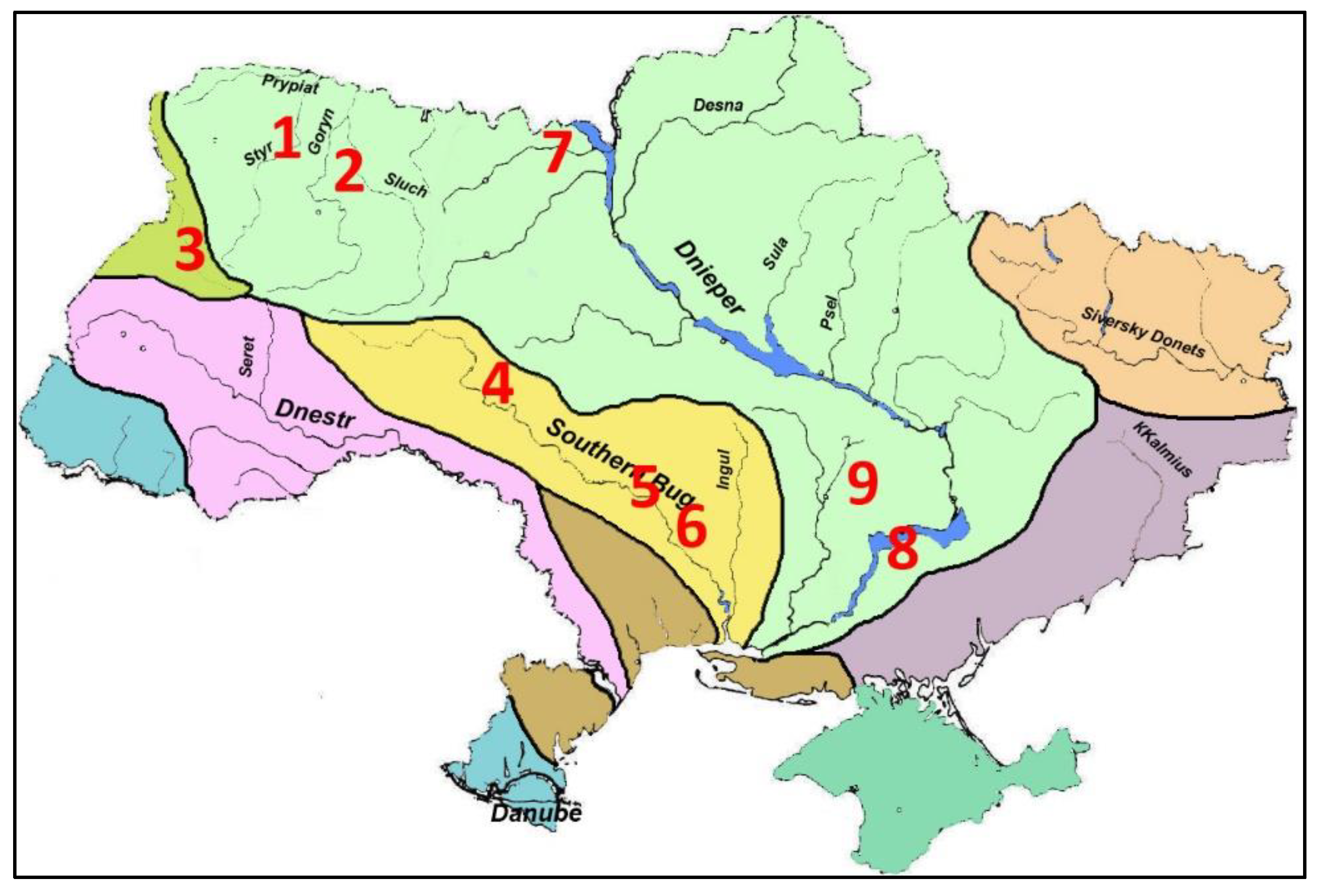
In studies of various water bodies of Ukraine, field data were obtained from cooling ponds of the Ukrainian Power Plants (
Figure 1,
Table 1). Ecotopic groups of hydrobionts were investigated: protistic periphyton and benthos (129 samples), phytoplankton, phytoepiphyton on filamentous algae (811), macrozoobenthos (32), and zooplankton (491). A sampling of the zoobenthos was carried out by the Ekman bottom grab with an area of sediments capture of 100 square centimeters. Sorting from bottom particles was carried out in the field, on waterbodies. A sampling of zooperiphyton was carried out from underwater substrates of bottom silt, gravel and sand using a scraper. The width of the blade was 5 centimeters. At a depth more than 0.5 m, the sampling was carried out using SCUBA equipment. Microphytoperiphyton samples were taken by washing from a certain area of substrates extracted from water from a depth of up to 0.5 m. Zooplankton samples were taken by filtering a certain amount of water through Apstein's plankton net, with cells of the network 80 μm. Samples were fixed in 4% formaldehyde. The composition and abundance of Protista were determined on live material; the remaining samples were analyzed in a fixed form in the laboratory. The calculated diversity and saprobity indices from Ukrainian material of
Table 1 were included in the construction of the diagrams as a whole or separately for ecological groups and waterbodies.
Diversity assessment was carried out separately: 1) for the richness of elements, taxonomic diversity (by the number of taxon’s in hydrobiological groups), expressed by the number of taxons, and 2) for the relative representation of cenopopulations in communities (by abundance or biomass), expressed by Shannon indices as:
where: N = common organisms abundance; s = species number; n
i = species number of each species; H, Shannon diversity index, bit.
The determination of saprobic indices was carried out according to the Pantle-Buck method in Sládeček's modification [
19]. Saprobity indices were obtained for each algal community as a function of the number of saprobic species and their relative abundances:
where
S is index of saprobity for algal community (unitless);
s is species-specific saprobity index;
n is the cell density of each species.
Recalculation of Sládeček saprobity indices into Watanabe saprobity indices was carried out according to the scale [
18,
20] for the subsequent inclusion of data in the empirical model.
3. Results and Discussion
3.1. Constructing of the Model of the Ecosystem Continuum
On the base of our long-term investigation of aquatic communities in Ukraine results (
Table 1), we summarized information and try to construct the theoretical model of the ecosystem continuum. Thus, the linkage between diversity and other indicators of communities has been considered repeatedly [
5,
11,
12,
21,
22,
23,
24]. These works are proposed that the decrease of anthropogenic pressure and pollution is considered as an improvement of the environment and vice versa. However, the stabilization of the conditions does not contribute to the achievement of maximum species diversity of communities [
25,
26]. In addition, the highest primary production not always determines the greatest diversity, but some of its average values [
12], because often the high productivity of producers is determined by one or two species, which reduces the diversity of the community.
Ten hypotheses about biodiversity have been formulated by [
13], and then their number reached many dozens [
21,
27]. Mostly of hypotheses relate exactly to the relationship between community diversity and the environment that it depends. At the same time, the concept of monotonous unimodal decrease or increase in diversity when certain conditions change prevails [
21,
23,
28] where structural diversity correlates with ecosystem entropy [
29] when lowest diversity reflects the highest entropy.
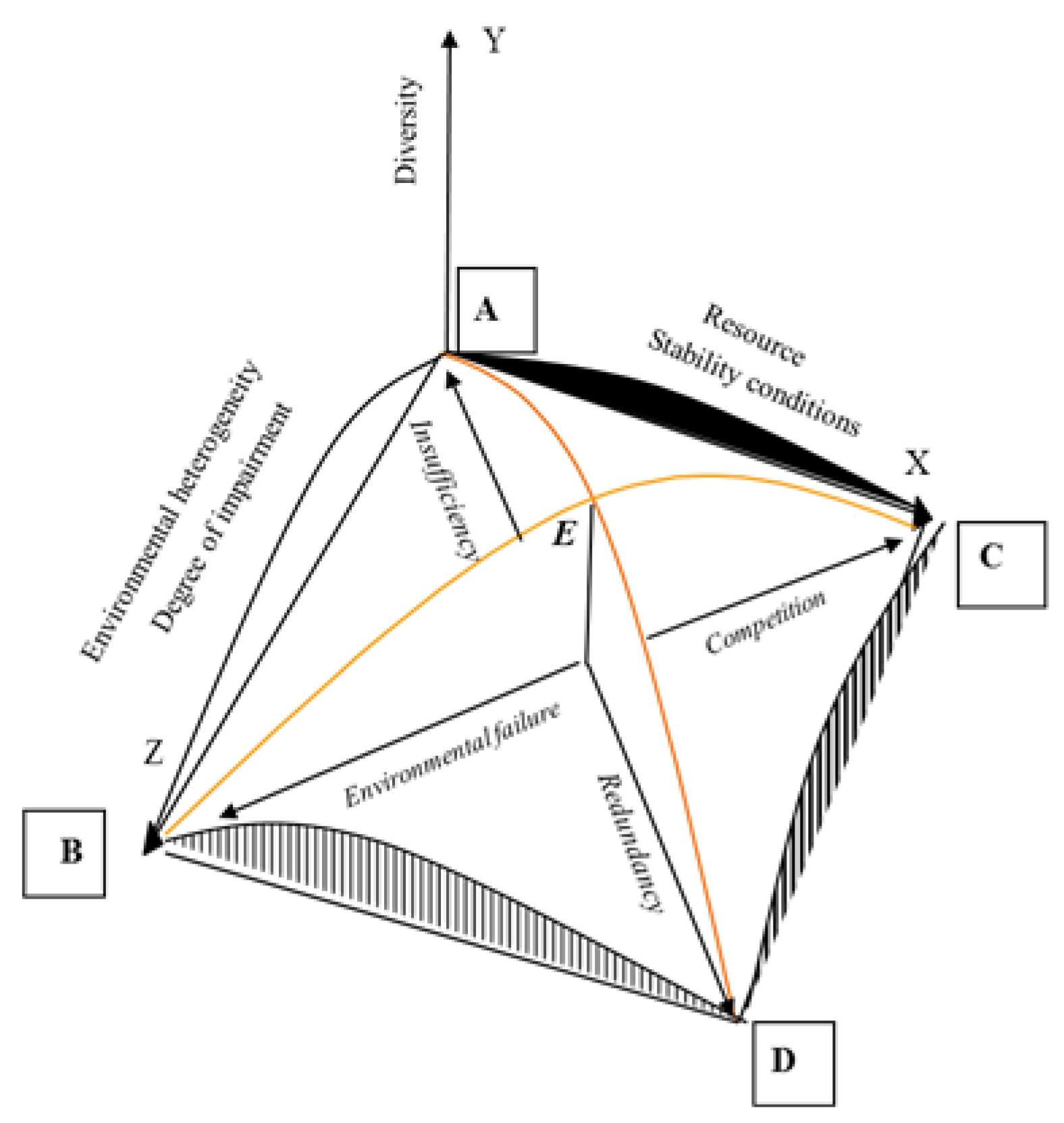
Thus, in our glance, diversity, like most characteristics of biological systems, forms according to the unimodal principle—decreases in two areas of pessimal conditions and increases in the optimal area. Factors do not act separately, but what happens when they are combined? In conditions of scarcity of resources, low stability, low heterogeneity of the environment, low level of disturbances (point A,
Figure 2), diversity is low.
The area of point B can be called the area of the most unfavorable conditions for life. The diversity here will be minimal due to the low values of richness and evenness. Ecosystems of highly urbanized areas, techno-ecosystems are located closest to ecosystems with such conditions. Maximum abundance of resources with maximum stability conditions and a minimum of disturbances and heterogeneity (point C) also does not represent a favorable combination for high diversity. Such conditions can be compared with the "flowering" of water bodies when it occurs with a combination of natural factors, that is, with minimal external influences. In conditions of high stability, diversity is no already controlled by physical environmental factors, and by biotic interactions—competitive displacement, the redistribution of the volume of ecological niches, high dominance of one or two species [
26].
Finally, the zone of maximum impact factors (point D), in which a high degree of disturbance is constant as much as possible and the resources are very abundant in the most heterogeneous biotope. As an example of this type of ecosystem, we can give the ecosystem of sewage treatment plants. The external influence here is maximum because the system is artificial, extremely high organic content, conditions are quite stable, and heterogeneity is increased by various methods of increasing the substrate dispersion.
Thus, the diversity of communities is minimal in the points ABCD, and increase to a maximum in point E. Therefore, the summit of the model corresponds to the average values of all factors. The continuum model factors changing can be interpreted as unimodal. The branching of the succession opportunities of the community so-called bifurcation stays out of the frame of this model. In the first glance, considering empirical data of changing natural communities of hydrobionts, we have to recognize that bifurcation is not observed in natural communities but if so, detailed study of the community structure data can help to clarify this question.
3.2. Bioindication of Environmental Conditions (Water Quality, Ecosystem State) and Diversity
An important problem of the application of diversity assessments is related to the bioindication of environmental quality. Since the structural and functional characteristics of communities are formed in accordance with habitat conditions, their change can be an indicator of changes in environmental conditions.
The use of species diversity indices (the Shannon index) showed that with the increasing pollution, the diversity of communities decreases [
12]. However, there is also data about the unimodal nature of changes in species diversity in the gradient of increasing trophy and pollution. The diversity is small both in oligotrophic conditions, a fairly clean environment, and in highly polluted. In the formal approach, this distribution makes it extremely difficult to assess the quality of the environment by diversity, since the values of the diversity index can be equal in completely different conditions [
18,
30].
The saprobity index as an indicator of organic pollution in our investigations changed with pollution loads, the structural Shannon index fluctuated also. It is important, that we calculate both indices on the base of the same data for the entire community. Indices of saprobity are calculated based on the same indicators as the Shannon index, that is, the indicator weight of the species and its abundance in the community, and it is a trophic view on the community, as opposed to only structural. However, the diversity of communities determined by the Shannon index is an indicator of the emergent properties of the biotic system. At the same time, approaches to analyzing the state of the ecosystem look more productive if different indicators of diversity are compared, such as species richness, structural indices of communities as well as trophic-related saprobity indices.
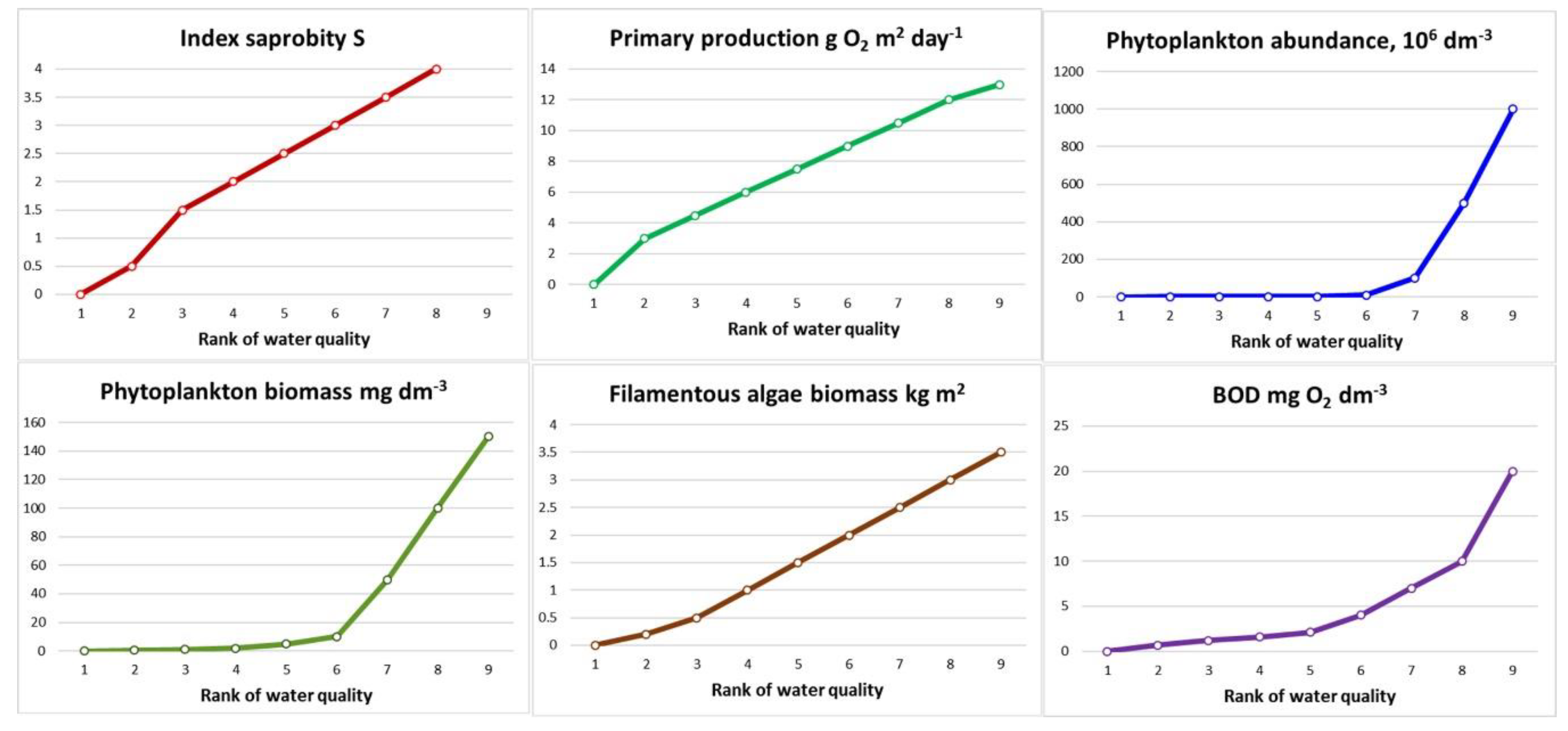
The advantage of reducing or increasing environmental quality indicators in the pollution gradient is that their numerical values correspond to the polluted zones, [
11,
12,
19] (
Figure 3,
Table 2) and are unimodal. In this case, the proposed symmetry of the reaction of the system structure in the areas of maximum and minimum pollution cannot always be unambiguously interpreted. Thus, assuming that "declining diversity to zero given that increasing pollution is a catastrophic stage of anthropogenic succession" [
18,
31], it is necessary to have at least unambiguous information about the direction of succession processes. This requires a comparison of at least two research results. It is best to have a long-term series of observations when a decrease of Shannon indices talks about community regression. At the same time, a decrease of the saprobity indices in the time series for a particular waterbody, and the increase in time the same indices of structural complexity talk about improving the state of the water body and about self-purification [
18,
32].
This brings us to a general view on the framework of those conditions in which the existence of water ecosystem is in principle possible.
3.3. Freshwater Ecosystem Model
Aquatic ecosystems can only form in a certain range of environmental variables that has been well demonstrated in the Sládeček model [
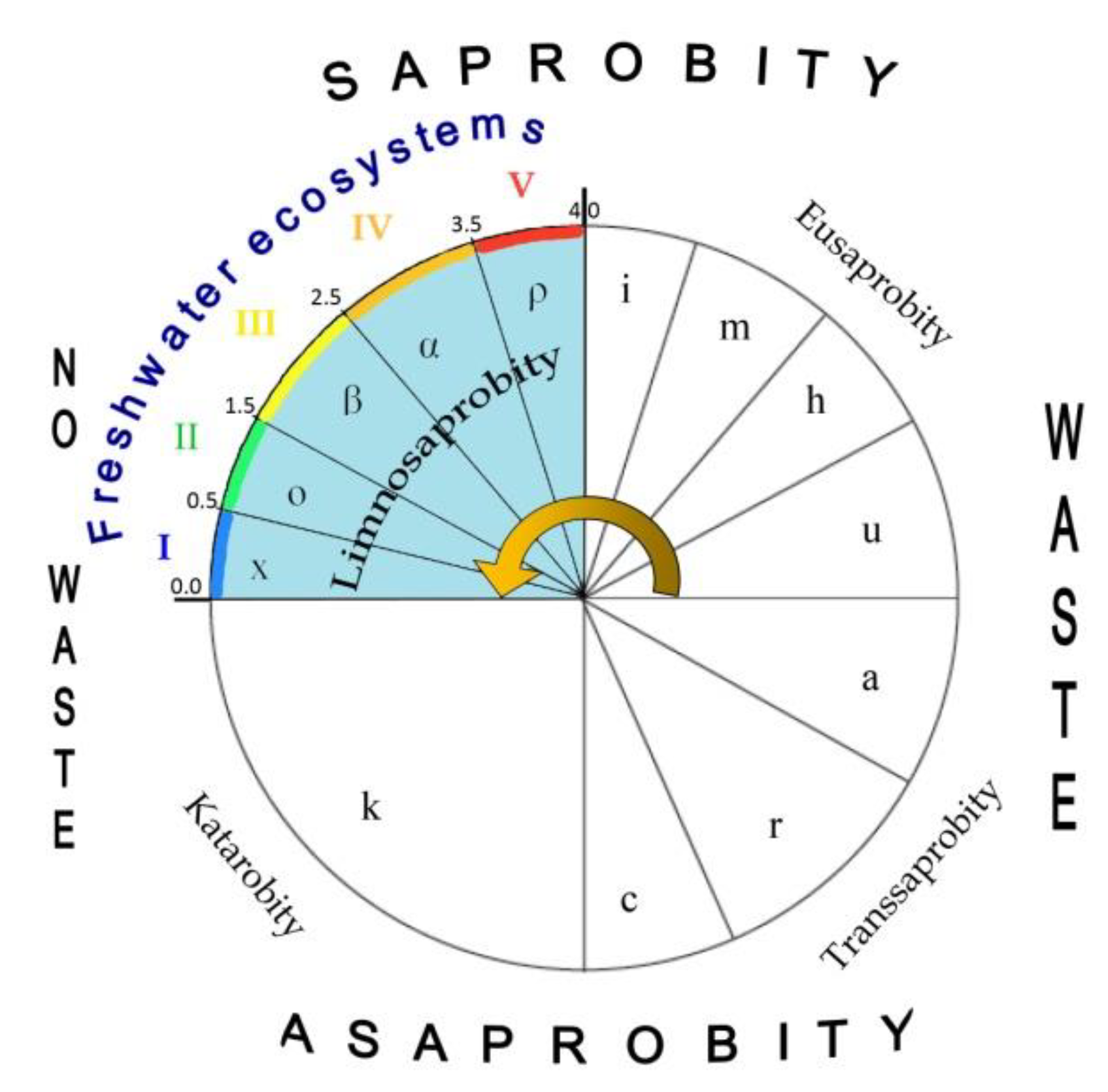
35]. V. Sládeček collected and analyzed a large amount of information concentrated at the Institute for Water Research, and developed the basic empirical dependences of the distribution of various biotic groups in accordance with the gradient of water indicators. The organization of aquatic biota in natural waters in the form of a trophic pyramid was the basis of his reasoning. In his system, the reactions of aquatic organisms of various taxonomic affiliations to changes in the parameters of the water in which they lived in nature were studied in detail. It turned out that natural water, in which the survival of photosynthetic organisms was noted, have limited parameters. Thus, the main property of the Sládeček’s model is the definition of the many water quality variables amplitudes from distilled water to the technical solutes. It is important to understand that aquatic ecosystems exist only within certain limits of environmental indicators of any possible [
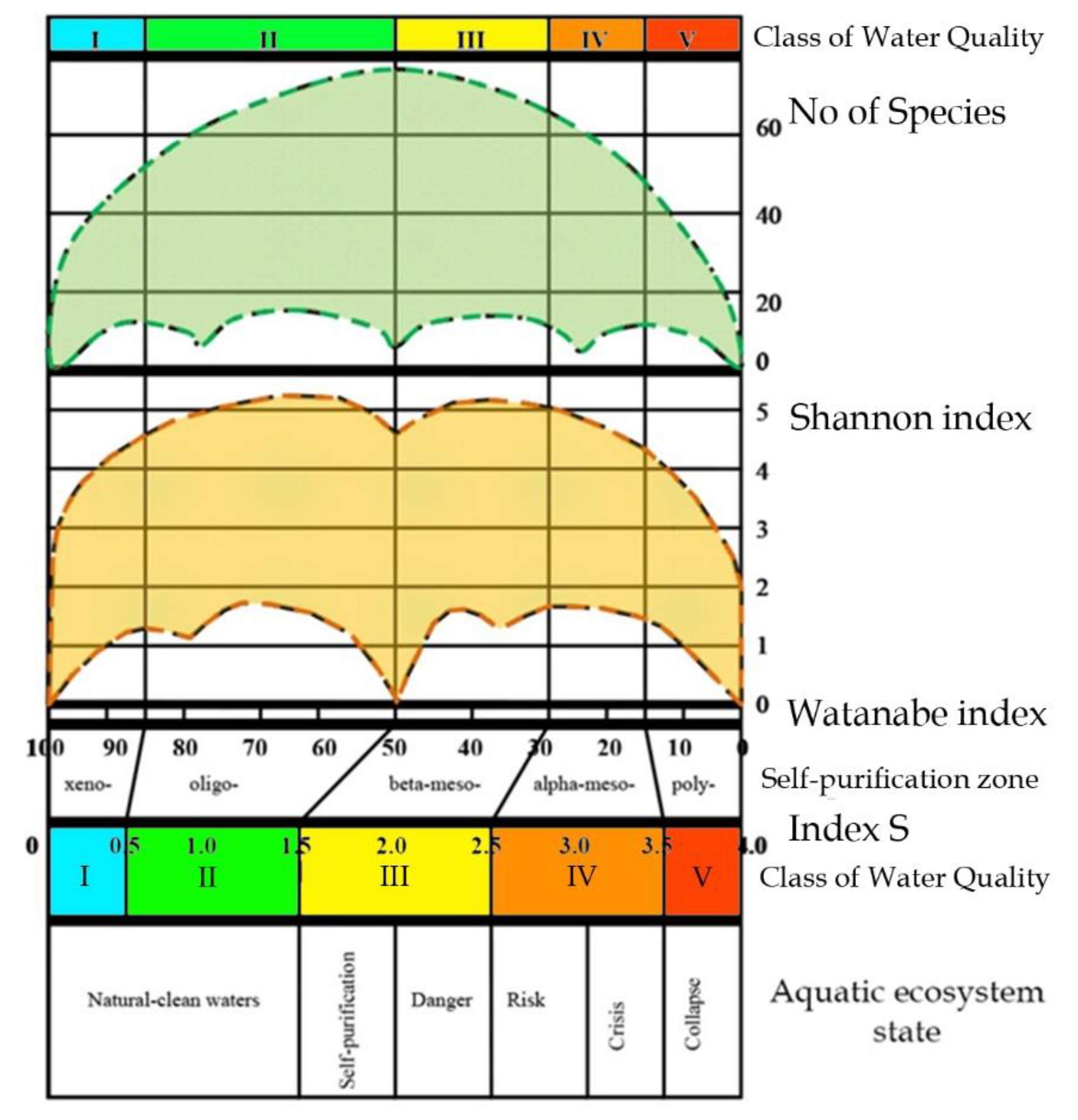
18], as can be seen from the Sládeček model shown in
Figure 4, equipped with self-purification zones, water quality classes, and EU color codes following
Table 2 [
36]. That is, an aquatic ecosystem based on photosynthetic organisms does not exist in any conditions, but only in the first quadrant (Limnosaprobity). The Saprobity S index is also included in the model and ranges from 0 to 4.
Data of the diversity and the communities structure of all ecological groups of hydrobionts can be used for bioindication purposes, although bioindication system by autotrophs with more than 8000 indicator taxa is the most developed [
4,
37,
38]. However, there is an opinion that the use of communities, for example, macrozoobenthos gives adequate results, which is related to certain stability of these groups [
39]. Determination of saprobity indices, taking into account the indicator role of individual species and their relative abundance, indicators of the diversity of communities, hold for both producers [
40] and consumers.
3.4. Empirical Modeling
To adapt our constructions of the dependences of diversity indicators on the scale of saprobity indices in our empirical model [
18], we give a scale of the relationship of the Sládeček and Watanabe saprobity indices and the correspondence of their intervals to Water Quality Classes (
Figure 5). The transition from one system of saprobity indices according to Sládeček to another, according to Watanabe, is described in [
18,
20,
37], and is due to the fact that the symmetry of full-scale structures looks clearer when the abscissa axis is represented by the Watanabe indices. In the full-scale of the Empirical Ecosystem Model can be seen that the Shannon index in the studied algae communities from the collection of the University of Haifa (orange field of dots) fluctuates between 0 and 5 and has a clearer border in the upper part of the dots field than in the lower one (
Figure 5). Symmetric bimodal distribution of a community structure index Shannon Index H can be recognized. This means that a community changes its structure in the trend of environmental variables [
19] in the full amplitude of ecosystem parameters based on photosynthetic organisms. It is necessary to pay attention to the fact that the values of the saprobity indices in the Sládeček and Watanabe systems are differently directed. In the Sládeček system, pollution increases with increasing S values from 0 to 4, while in the Watanabe system, the saprobity index is lower in polluted waters and increases to 100 in naturally pure waters. Thus, part of field H in
Figure 5 with an amplitude of Watanabe indices from 40 up to 100 characterizes natural ecosystems whose waters are either clean or have self-cleaning mechanisms. The range of indices Watanabe 30–40 can be marked as dangerous for the structure of the community and the ecosystem as a whole. A community with Watanabe indices in the range of 20–30 is at risk and with indices of 15–20 at a critical stage. If community saprobity indices are in the range of 0–15, the degradation of its state develops very quickly and the ecosystem can collapse. A detailed description of the model with a change in the species composition of algal communities is given in [
18].
It should be noted that in our followed constructions axis of attitude to water quality classes, associated with a unimodal distribution of environmental and trophic-related parameters remained constant scale (
Table 2,
Figure 3). In the same time, saprobic indices according to Sládeček could be replaced by other parallel Watanabe indices, which brings the logic of our presentation closer to the empirical modeling of the results obtained. Thus, we constructed the distribution of Shannon diversity indices and species richness for algal communities within the full scale of saprobity indices [
18,
41] based on our data from more than 2000 samples.
Figure 5 shows that the field of distribution points of structural indicators (orange field) is bimodal, while the indicators of species richness of communities (green field) represent a unimodal distribution. The axis of symmetry of both distributions runs in the range of the Sládeček saprobity index 1.5 or Watanabe 50. That is, in the empirical model [
18], two symmetrical wings of the distribution of points of structural indicators according to trophic indicators of saprobity can be attributed to positive and negative changes in the ecosystem, which reflects bimodality in assessing its state. While an improvement in ecosystem status is postulated with increasing diversity, more complex relationships can be observed in the model. The use of only structural indicators complicates and makes the assessment itself sometimes inadequate or impossible since the minimum Shannon indices can relate to both naturally pure and heavily polluted water bodies. However, if the structural indicators are normalized along the axis of increase (or decrease) of the saprobity indices, one can see a regular bimodal distribution, which can be interpreted in connection with a change in the environmental and production parameters of ecosystems.
3.5. Zoobenthos Community Diversity Indicators
We have conducted studies of zoobenthos communities in various water bodies of Ukraine (
Table 1) in order to establish the relationship between indicators of diversity and saprobity. The diversity indices of the zoobenthos communities and the saprobity indices varied within rather large limits and established in
Table 3.
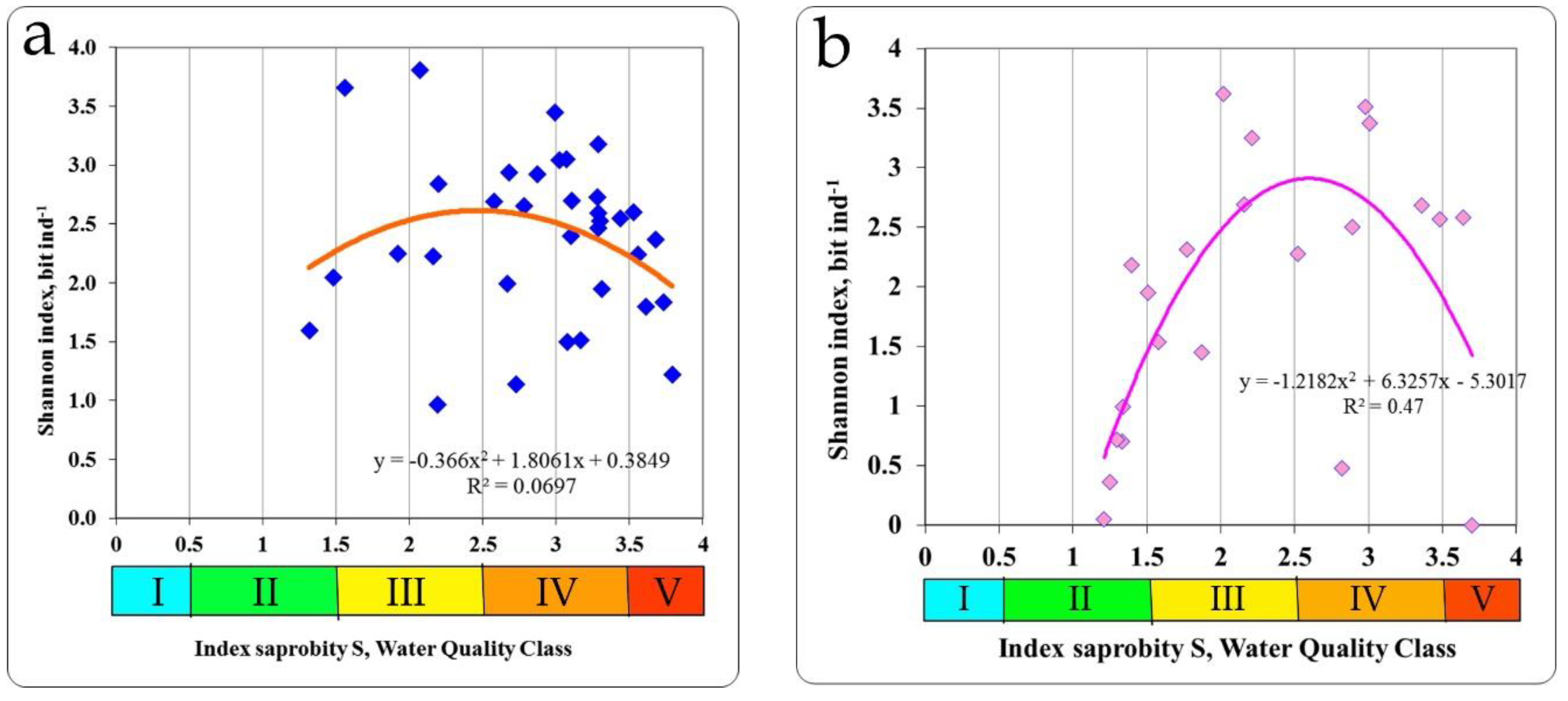
In the zone of the Khmelnitsky NPP, investigations were conducted on the Goryn and Viliya rivers and in the cooling pond of the Khmelnitsky NPP. The relationship between the saprobity index S and the Shannon index was found as unimodal. Therefore, the summit of the trend line of Shannon diversity index was 2.507 bit ind.
-1 with an index of saprobity S = 2.5 (
Figure 6a), the same distribution for the taxonomic diversity (summit of the trend line is 2.100 bit species
−1) was with an index of saprobity S = 2.90 (
Table 3).
The reservoir of the pumping station, the channel in the cooling system of an NPP were investigated in the area of the RNPP the Styr River. The diversity of biotopes was much higher than in the Goryn and Vilia rivers. The saprobity index S by zoobenthos was in the range of 1.21–3.70 and the Shannon diversity indices in the range of 0–3.622 for distribution of which has been found the unimodal character. The value of the Shannon index for species diversity at the summit of trend line was 2.900 bit ind.
−1 and corresponded to a saprobity index S value of 2.62 (
Figure 6b). At the same value of the index of saprobity S taxonomic diversity also reached a maximum with 2.300 bit species
−1 (
Table 3).
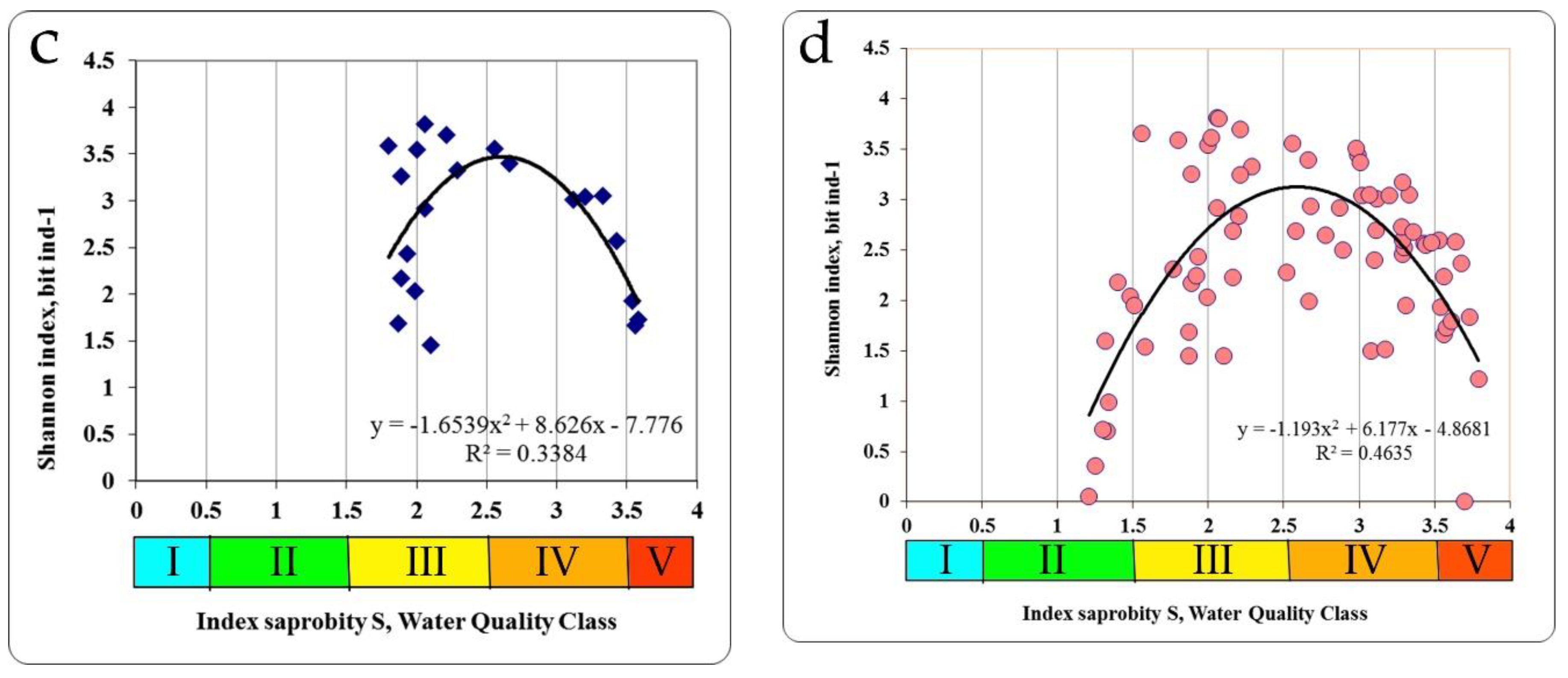
In the Chernobyl NPP cooling pond and in the floodplain lakes of the Chernobyl NPP zone, at unimodal dependence between the indicators of the saprobity index S and the Shannon diversity indices by zoobenthos the maximum of the last in the extremum point of trend line (3.375 bit ind.
−1) was found at the saprobity index S = 2.60 (
Figure 6c). The structure of zoobenthos communities changed in the gradient of the saprobity index S (
Figure 6d) for all summarized data. Thus, at small values of the saprobity index S and the Shannon diversity index in the benthic communities of the Styr River, a low number of species was registered with a conspicuously high degree of dominance of one or two species. These were mostly psammophilous species, preferring clean, flowing waters (
Table 4).
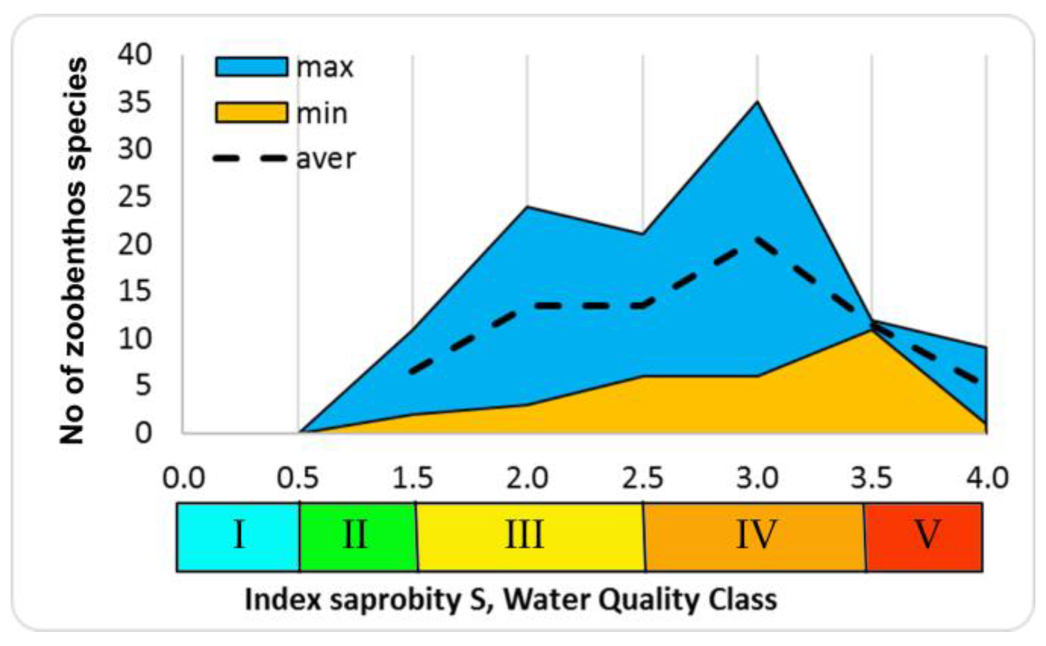
The number of species increases at increasing indices of saprobity and diversity in studied zoobenthos communities of Ukraine. Communities become polydominant at the dominance of rheophilic oligo-beta-mesosaprobic species (Trichoptera larvae, Chironomidae larvae). At a saprobity index of 2.80, pelophilic alpha-polysaprobes appear in the dominant group while preserving the polydominant community structure, and at an increase of the index of saprobity above 3.00, a decrease of the number of species and decrease of diversity index were noted. Zoobenthos communities become monodominant at the significant prevalence of pelophilic alpha- polysaprobes. Thus, the change in the diversity index in the gradient of the saprobity index is associated with significant changes in the structure of zoobenthos in studied communities. The greatest richness is noted in the alpha'-mesosaprobic zone, rank 6, Class IV of water quality in the Sládeček model (
Figure 7).
There is a concept about the direct relationship between species richness and environmental quality indicators [
39]. This concept is based on empirical data, suggesting that the degradation of the quality of the environment leads to the impoverishment of communities, decrease diversity and species richness. There is also a point of view that this dependence persists throughout the whole range of organic pollution, (corresponding to the first quadrant of the model Sládeček [
35] (
Figure 4). In the distribution of relative abundance or evenness aspect, it is known that at strong organic pollution, the role of a few abundant species and groups increases. This assumption follows from the analysis of the distribution over the partial, non-full scale of the pollution gradient (or trophic load) in the water ecosystem. We supposed that there is an inverse correlation between the indicators of diversity and saprobity indices. Because the absolute values of the index of diversity, as shown above, are decreased in the area of both small and large values of the index of saprobity (
Figure 5) as well as in the central part of the model when the saprobity indices are about 1.5, it is possible to search of indicators of diversity that are characteristic for waterbodies of given region [
43] or even for individual water bodies for future monitoring.
However, attention should be paid to the fact that the saprobity indices S calculated for the consumer communities studied by us in Ukraine do not cover the entire possible range from 0 to 4, as in
Table 2 and in the model of Sládeček, but only part of it, with S = 1.5–4.0. It represents only one part of the full distribution, the right wing of the Empirical model.
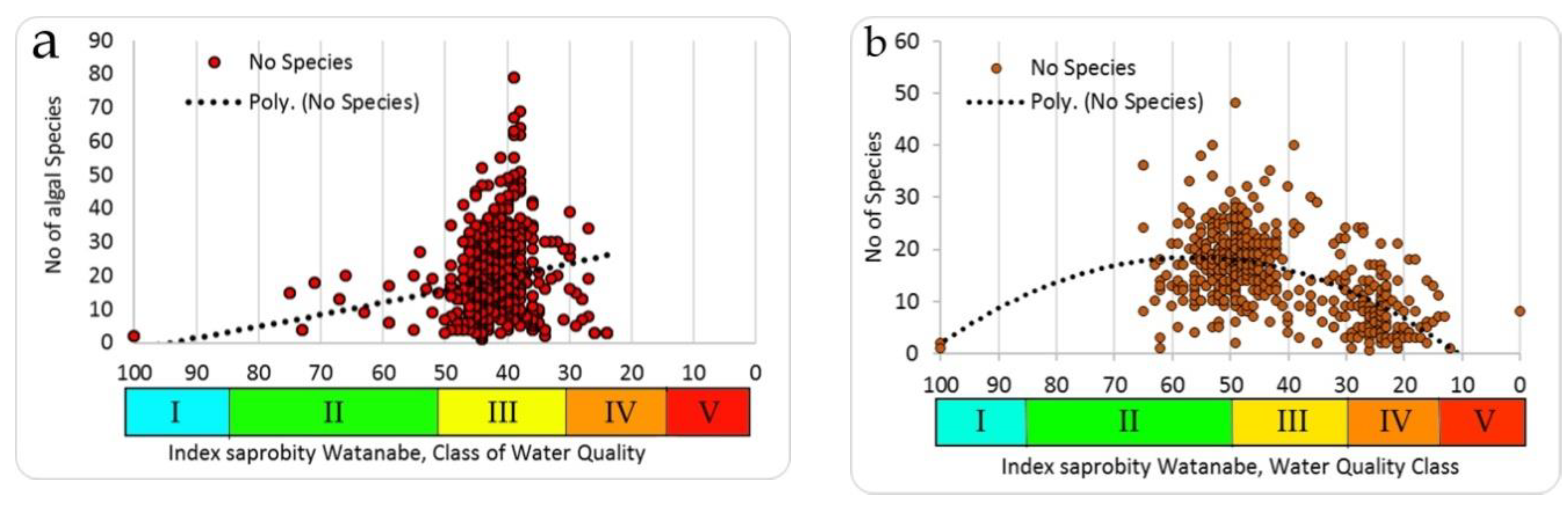
3.6. Comparison of Producers and Consumers’ Diversity Indicators
Comparing our data of species richness by producers and consumers (
Figure 8a,b), it is clear that the number of species in the full scale of the saprobity index Watanabe for producers (
Figure 8a) and consumers (
Figure 8b) differs noticeably in the coverage of the scale of the saprobity indices. The producers (algae) of water bodies that have been investigated are more diverse in terms of species richness in the zone of Water Quality Class III, while the maximal number of species of consumers is shifted to the zone of the class of water quality IV.
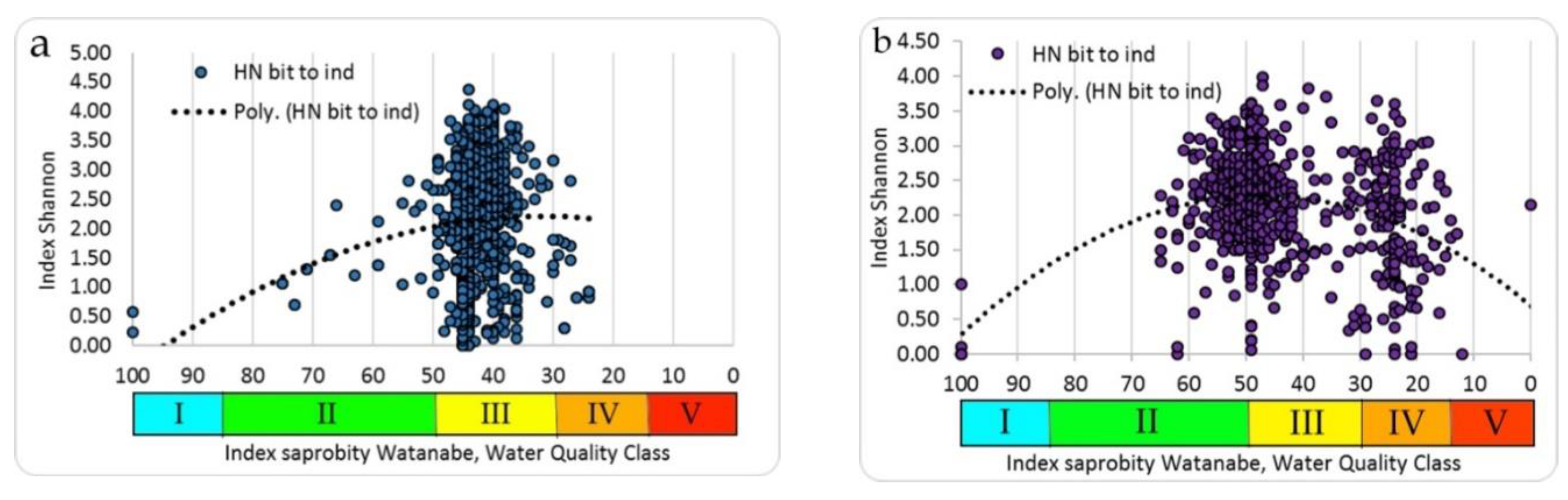
A similar construction for the distribution of Shannon species diversity indices for the same studied communities showed that the algae community by the structure are more closely grouped and are also confined to the III class of water quality (
Figure 9a) than the communities of consumers, whose Shannon indices vary widely and also cover the more trophically loaded part (
Table 2) of the full scale of saprobity indices (
Figure 9b).
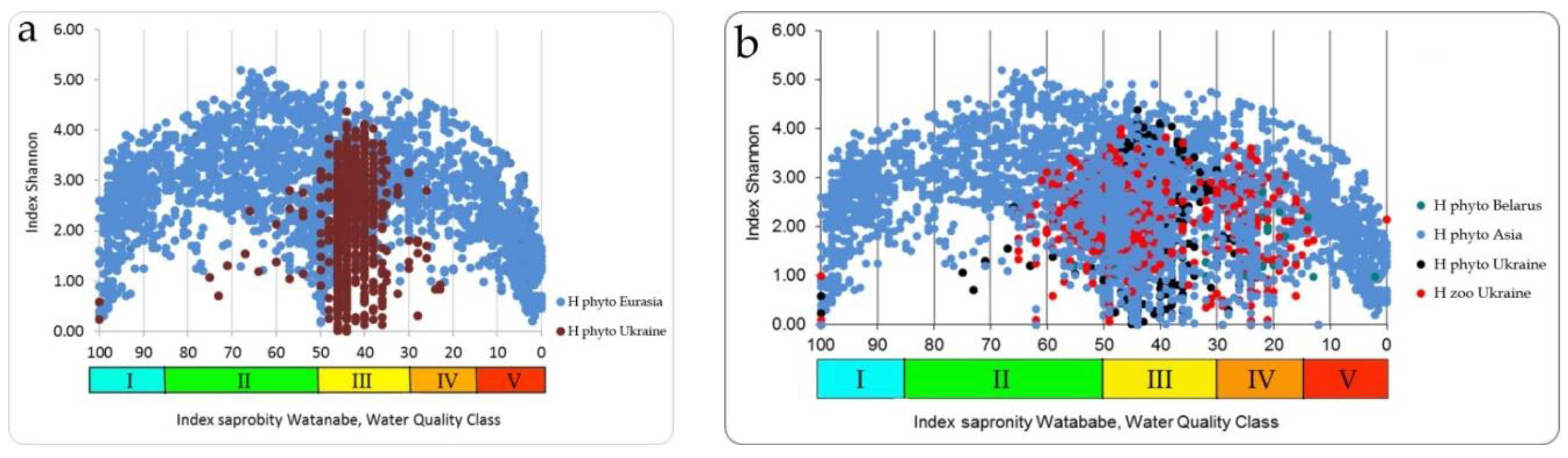
The same distributions of the algae species richness (upper green field) and Shannon indices (lower orange field) in the Empirical Model were constructed over indices of Watanabe. Thus, species richness distribution for more than two thousand communities of Eurasia (
Figure 5) looks like unimodal with the maximal number of species in the range of saprobity indices of Watanabe about 50, and in Sládeček scale about 1.5 [
18].
The Ukrainian phytoplankton and zoobenthos communities’ species richness and Shannon indices values (
Figure 8,
Figure 9) are nested into the species richness field of dots (
Figure 5) of the Empirical Model as well as into the Shannon index field of dots (
Figure 10).
In the Empirical Model in
Figure 5, represent connecting the water pollution indices with diversity indices and species richness of algal communities. As an indicator of diversity, Shannon's information function is used; the level of anthropogenic impact is estimated by saprobity indices using the methods of Sládeček and Watanabe. It is not only empirical but also successional model because pollution indices Watanabe and S corresponds to the regularly changing chemical and biological variables [
19] over the first quadrant of
Figure 4.
To interpret the obtained results for water bodies in Ukraine, it is important to take in account that with a unidirectional increase in the level of impact, reversibility of the development of biological diversity is observed at the first stages of the progressive development of an algal community. Then, after the crisis phase—a fracture of the empirical curve—in the succession stage of regressive development there is a decrease in the indices of diversity in a condition of continuing increase in trophic load.
The postulate of the dependence of community development from the availability of resources seems unimodal and understandable like in the Model of the ecosystem continuum (
Figure 2). However, this only holds true in a narrow range of available resources. The dependence turns out to be bimodal if changes are considered over the full scale of the resource [
3]. This is consistent with our constructions for structural indices and community saprobity indices within the Empirical Ecosystem Model [
18]. Data from the Ukrainian analyzed material is nested into the Empirical model without any deviations or excesses.
Discussion of the regularities in which the community changes leads many authors to the conclusion that the structure of communities after removing impact can change in two ways: continuing the growth of diversity or lowering the diversity along the same curve but in the opposite direction. The assumption of such branching of the succession opportunities of the community is called bifurcation. Considering empirical data and changing natural communities of hydrobionts, we have to recognize that bifurcation is not observed in natural algal communities. Perhaps, for a double direction of development of communities, the symmetry of structures is better accepted as the "natural" and "anthropogenic" stages of succession. On our model [
18], it can be seen that the right and left-wing of the figure have similar outlines. Thus, development does not go in the opposite direction, but in the progressive direction on the model, as the transition from the left wing to the right and it is confirmed by the species changes in communities. Since the biotic part of the ecosystem is built according to the law of the trophic pyramid, it can be concluded that our model is applicable for assessing the state of the aquatic ecosystem as a whole. Moreover, our study demonstrated the difference in the distribution of diversity indices for autotrophic communities and communities of different consumers in the same water body with parallel sampling and counting. The consumer community demonstrates the highest rates of saprobity than phytoplankton, and, consequently, overestimate the assessment of organic pollution in comparison with autotrophs.
4. Conclusions
Diversity in biological systems is considered in various aspects as richness, evenness, diversity and dominance of functional groups [
1,
41] depending on the task posed to a specific analysis. The diversity indices calculated for each type of analysis ultimately reflect the relationship between the various aspects of assessing community structure in relation to the gradient of hydrochemical or climatic indicators of the environment. Only two models by Sládeček and Watanabe [
18,
35] cover the entire possible range of environmental indicators in which the existence of an aquatic ecosystem is possible.
Our analysis of the relationships the Shannon indices in communities of the Ukrainian waterbodies and their environment, we are revealed that calculated diversity indices, as well as species richness for phytoplankton communities, were fully nested to the distribution of same indices field in the Empirical Ecosystem Model. The study of the structural indices distribution in the water bodies of Ukraine let us given attention to the discussion about the bifurcation in the successional changes of the both, autotrophs and heterotrophs communities. Whereas the calculated diversity indices were nested into the Empirical model, it help us to conclude that successional stage of the consumer communities can be interpreted as in anthropogenic stage, but indices of autotrophs can characterize studied waterbodies communities as stay on the intermediate stage of succession, in so-called point of bifurcation.
Some new in our constructions and comparisons are the differences in responses of communities of the first (algae) and second (animals) trophic levels on the same organic loads in the studied water bodies of Ukraine. It is important to know that the water quality assessments by zooplankton and zoobenthos are estimates overestimate the level of organic pollution in the water body compared with estimates by the first trophic level organisms. It can be taken into account in purpose of the monitoring system construction and the classification of water quality standards.
In conclusion, can be remarked that the problem of relationships of community diversity and its distribution over the trophic-related variables of the ecosystem is rather far from exhausting and need our following attention for its study. It seems to us that the question of the relationship between diversity indicators of communities and environmental conditions is still far from being resolved and will require further research.
Author Contributions
Conceptualization, A.P. and S.B.; Data curation, A.P. and S.B.; Formal analysis, A.P. and S.B.; Investigation, A.P. and S.B.; Methodology, A.P. and S.B.; Project administration, A.P. and S.B.; Resources, A.P. and S.B.; Software, A.P. and S.B.; Supervision, A.P. and S.B.; Validation, A.P., S.B., T.N. and A.S.; Visualization, A.P. and S.B.; Writing – original draft, A.P., S.B., T.N. and A.S.; Writing – review & editing, A.P. and S.B.
Funding
This research received no external funding.
Acknowledgments
This work was partly supported by the National Academy of sciences of Ukraine, project N1230-2019. This work was partly supported by the Israel Ministry of Aliyah and Integration.
Conflicts of Interest
The authors declare no conflict of interest.
References
- Gilyarov, A.M. Relationship of biodiversity with productivity - science and politics. Priroda, 2001, 2, 20–24. (In Russian) [Google Scholar]
- Cardinale, B.J.; Gross, K.; Fritschie, K.J.; Flombaum, P.; Fox, J.W.; Rixen, C.; van Ruijven, J.; Reich, P.B.; Scherer-Lorenzen, M.; Wilsey, B.J. Biodiversity simultaneously enhances the production and stability of community biomass, but the effects are independent. Ecology 2013, 94, 1697–1707. [Google Scholar] [CrossRef] [PubMed] [Green Version]
- Alexander, T.J.; Vonlanthen, P.; Seehausen, O. Does eutrophication-driven evolution change aquatic ecosystems? Phil. Trans. R. Soc. B 2017, 372, 20160041. [Google Scholar] [CrossRef] [PubMed] [Green Version]
- Barinova, S. Essential and practical bioindication methods and systems for the water quality assessment. Int. J. Environ. Sci. Natural Resources 2017, 2, 1–11. [Google Scholar] [CrossRef]
- Protasov, A.A. Biodiversity and its assessment. Conceptual diversicology; IНB NASU Publisher: Kiev, Ukraine, 2002; p. 105. (In Russan) [Google Scholar]
- Jones, C.G.; Lawton, J.H.; Shachak, M. Organisms as ecosystem engineers. Oikos, 1994, 69, 373–386. [Google Scholar] [CrossRef]
- Thompson, P.L.; Davies, T.J.; Gonzalez, A. Ecosystem functions across trophic levels are linked to functional and phylogenetic diversity. PLoS ONE 2015, 10, e0117595. [Google Scholar] [CrossRef]
- Dochin, K. Functional and morphological groups in the phytoplankton of large reservoirs used for aquaculture in Bulgaria. Bulgarian J. Agric. Sci. 2019, 25, 166–176. [Google Scholar]
- Legras, G.; Loiseau, N.; Gaertner, J.-C. Functional richness: Overview of indices and underlying concepts. Acta Oecologica 2018, 87, 34–44. [Google Scholar] [CrossRef] [Green Version]
- Protasov, A.A. Life in the hydrosphere. Essays on General Hydrobiology; Academperiodika: Kiev, Ukraine, 2011; p. 704. (In Russan) [Google Scholar]
- Alimov, A.F. Elements of the theory of functioning of water ecosystems; Nauka: St. Petersburg, Russia, 2000; p. 147. (In Russian) [Google Scholar]
- Alimov, A.F.; Golubkov, S.M.; Bogatov, V.V. Production hydrobiology; Nauka: St. Petersburg, Russia, 2013; p. 457. (In Russian) [Google Scholar]
- Pianka, E. Evolutionary Ecology; Mir: Moscow, Russia, 1981; p. 399. (In Russian) [Google Scholar]
- MacArthur, R.H. On the relative abundance of species. Amer. Natur. 1960, 94, 25–36. [Google Scholar] [CrossRef]
- Rosenberg, G.S. Informational index and diversity: Boltzmann, Kotelnikov, Shannon, Weaver. Bulletin Samar. Luka: Probl. Reg. Global Ecology 2010, 19, 4–25. (In Russian) [Google Scholar]
- Cui, S.; Li, X.; Voss, L.J. Using permutation entropy to measure the electroencephalographic effects of sevoflurane. Anesthesiology 2008, 109, 448–456. [Google Scholar]
- Eguiraun, H.; López-de-Ipiña, K.; Martinez, I. Application of Entropy and Fractal Dimension Analyses to the Pattern Recognition of Contaminated Fish Responses in Aquaculture. Entropy 2014, 16, 6133–6151. [Google Scholar] [CrossRef] [Green Version]
- Barinova, S.S. Empirical Model of the Functioning of Aquatic Ecosystems. Int. J. Oceanography Aquaculture 2017, 1, 1–9. [Google Scholar] [CrossRef]
- Barinova, S. On the classification of water quality from an ecological point of view. Int. J. Environ. Sci. Nat. Res. 2017, 2, 1–8. [Google Scholar] [CrossRef]
- Barinova, S.S.; Medvedeva, L.A. Atlas of Algae-Indicators of Saprobity (Russian Far East); Dal’nauka: Vladivostok, Russia, 1996; p. 364. (In Russian) [Google Scholar]
- Kratochwil, A. (Ed.) Biodiversity in Ecosystems: Principles and Case Studies of Different Complexity Levels; Kluwer Academic Publ.: Dordrecht, Boston, London, 1999; p. 218. [Google Scholar]
- Midgley, G.F. Biodiversity and Ecosystem Function. Science 2012, 335, 174–175. [Google Scholar] [CrossRef] [PubMed]
- Whittaker, R.H. Evolution and measurement of species diversity. Taxon 1972, 21, 213–251. [Google Scholar] [CrossRef]
- Hubalek, Z. Measures of species diversity in ecology: An evaluation. Folia Zool. 2000, 49, 241–260. [Google Scholar]
- Connel, J. Diversity in tropical rainforests and coral reefs. Science 1978, 199, 1302–1310. [Google Scholar] [CrossRef]
- Ward, J.V.; Tockner, K. Biodiversity: Towards a unifying theme for river ecology. Freshwater Biol. 2001, 46, 807–819. [Google Scholar] [CrossRef]
- Schaefer, M. The diversity of the fauna of two beech forests: Some thoughts about possible mechanisms of causing the observed patterns. In Biodiversity in Ecosystems: Principles and Case Studies of Different Complexity Levels; Kratochwil, A., Ed.; Kluwer Academic Publ.: Dordrecht, Boston, London, UK, 1999; pp. 39–57. [Google Scholar]
- Mirkin, B.M. What is the Plant Community; Nauka: Moscow, Russia, 1986; p. 164. [Google Scholar]
- Good, I.J. The population frequencies of species and the estimation of population parameters. Biometrika 1953, 40, 237–264. [Google Scholar] [CrossRef]
- Carlander, K.D. The standing of clop of fish in lakes. J. Fisheries Res. Board Canada 1955, 12, 543–570. [Google Scholar] [CrossRef]
- Barinova, S.S.; Medvedeva, L.A.; Anisimova, O.V. Algae as Indicators of Environmental Quality; Institute Nature Conservation Press: Moscow, Russia, 2000; p. 150. (In Russian) [Google Scholar]
- Barinova, S. Algal diversity dynamics, ecological assessment, and monitoring in the river ecosystems of the eastern Mediterranean; Nova Science Publishers: New York, NY, USA, 2011; 363p. [Google Scholar]
- Romanenko, V.D.; Oksiyuk, O.A.; Zhukinsky, V.N.; Stolberg, F.V.; Lavrik, V.I. Ecological Assessment of the Impact of Hydrotechnical Construction on Water Bodies; Naukova Dumka: Kiev, Ukraine, 1990; p. 256. (In Russian) [Google Scholar]
- Felföldy, L. The Biological Classification of Water Quality; 4th revised edition (A biológiai vízminősítés); Vízügyi Hidrobiológia, 16. VGI: Budapest, Hungary, 1987; p. 263. (In Hungarian) [Google Scholar]
- Sládeček, V. System of water quality from biological point of view. Erg. Limnol. 1973, 7, 1–218. [Google Scholar]
- Common Implementation Strategy for the Water Framework Directive (2000/60/EC). Guidance Document n. 9. Implementing the Geographical Information System Elements (GIS) of the Water Framework Directive; European Communities: Luxembourg, 2003; p. 156. [Google Scholar]
- Barinova, S.S.; Medvedeva, L.A.; Anisimova, O.V. Diversity of Algal Indicators in the Environmental Assessment; Pilies Studio Publisher: Tel Aviv, Israel, 2006; p. 498. (In Russian) [Google Scholar]
- Barinova, S.; Fahima, T. The Development of the a World Database of Freshwater Algae-Indicators. J. Environ. Ecology 2017, 8, 1–7. [Google Scholar] [CrossRef] [Green Version]
- Semenchenko, V.P. Principles and Systems of Bioindication of Flowing Waters; Orech Publisher: Minsk, Belarus, 2004; p. 125. (In Russian) [Google Scholar]
- Barinova, S.S.; Bilous, O.P.; Tsarenko, P.M. Algal Indication of Water Bodies in Ukraine: Methods and Prospects; Publishing House of Haifa University: Haifa, Israel; Kyiv, Ukraine, 2019; p. 367. (In Russian) [Google Scholar]
- Bakanov, A.I. Using the characteristics of zoobenthos diversity for monitoring the state of freshwater ecosystems. In Monitoring, Biodiversity; IPEE RAS Press: Moscow, Russia, 1997; pp. 278–282. (In Russian) [Google Scholar]
- Stevens, R.D.; Cox, S.B.; Strauss, R.E.; Willig, M.R. Patterns of functional diversity across an extensive environmental gradient: Vertebrate consumers, hidden treatments and latitudinal trends. Ecol. Lett. 2003, 6, 1099–1108. [Google Scholar] [CrossRef]
- Protasov, A.A.; Silayeva, A.A. On the assessment of the quality of the environment in terms of the diversity of communities of hydrobionts. Sci. Notes Ternopil State Pedagog. Univ. Ser. Biol. 2005, 3, 365–367. [Google Scholar]
© 2019 by the authors. Licensee MDPI, Basel, Switzerland. This article is an open access article distributed under the terms and conditions of the Creative Commons Attribution (CC BY) license (http://creativecommons.org/licenses/by/4.0/).


