
Detecting Pre-Analytically Delayed Blood Samples for Laboratory Diagnostics Using Raman Spectroscopy
 , and
, and
Abstract
:1. Introduction
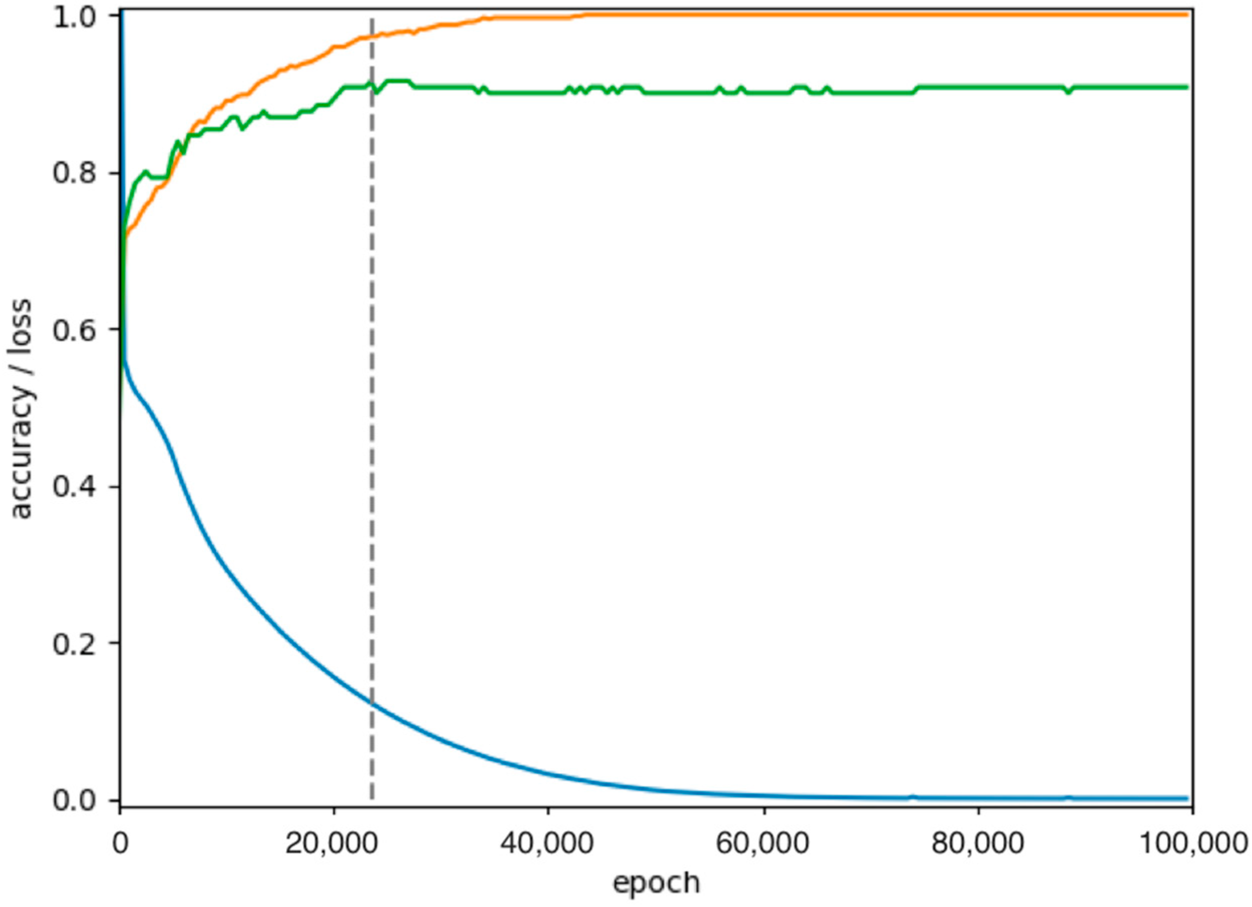
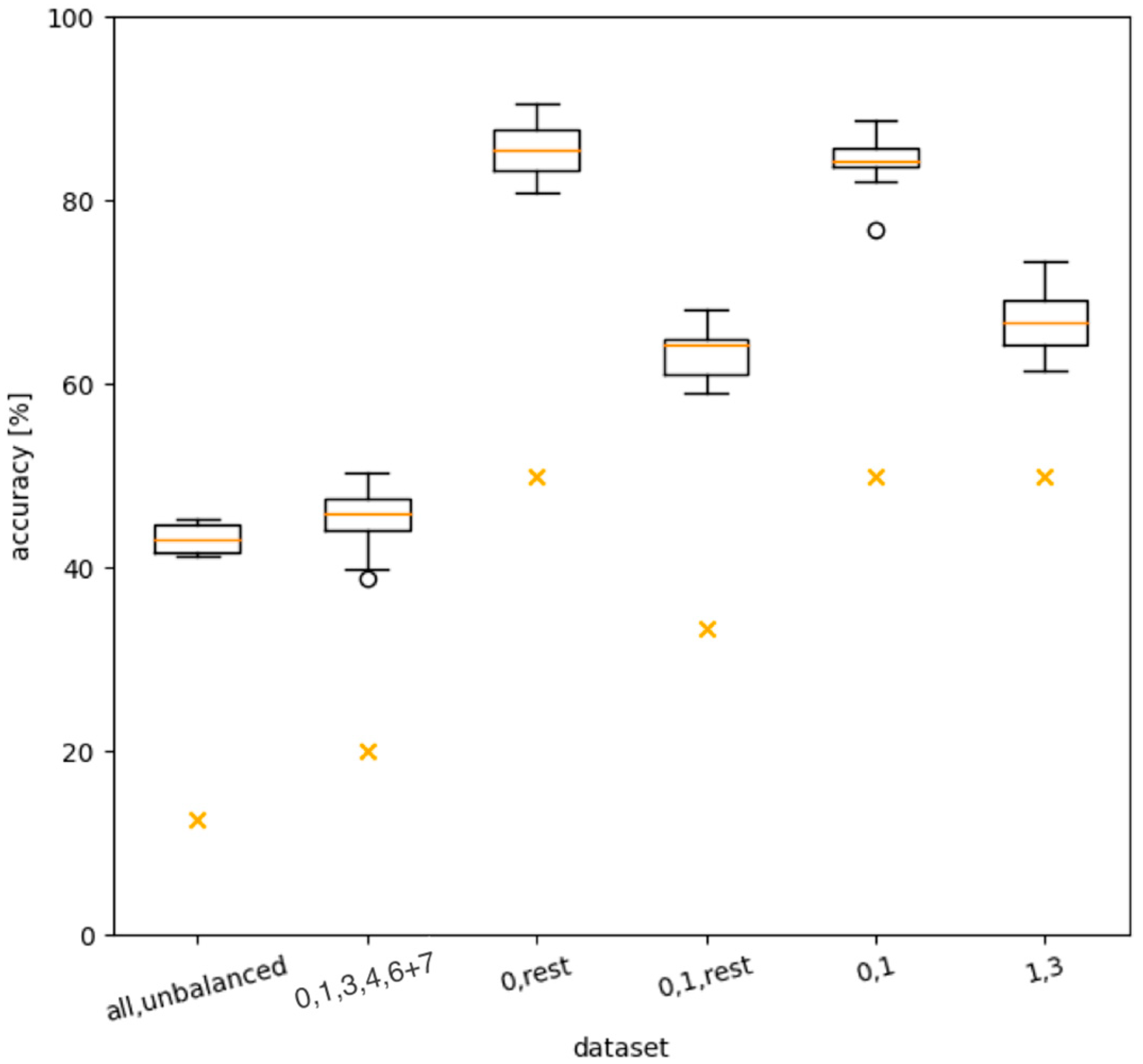
2. Results
3. Discussion
4. Materials and Methods
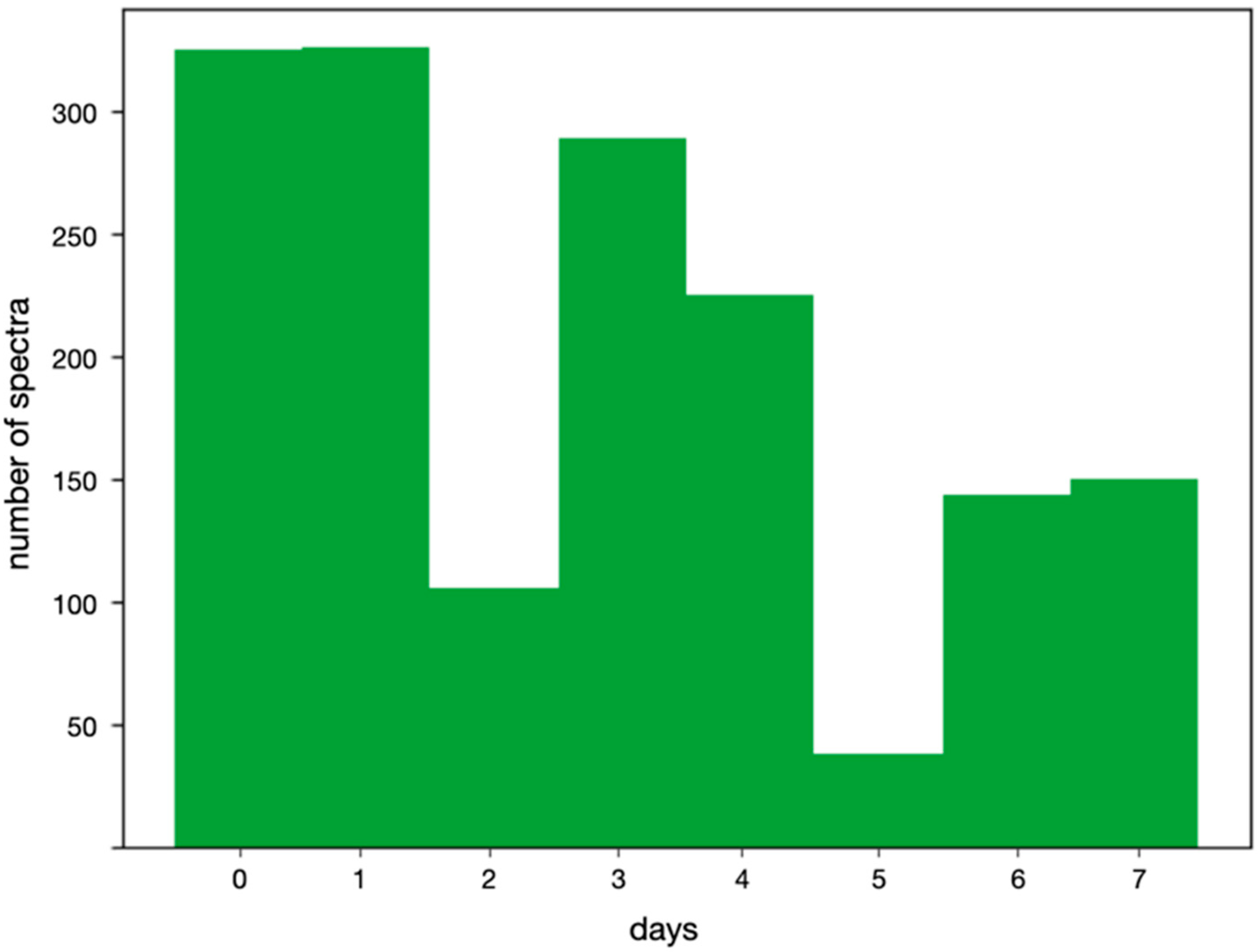
4.1. Samples and Spectra
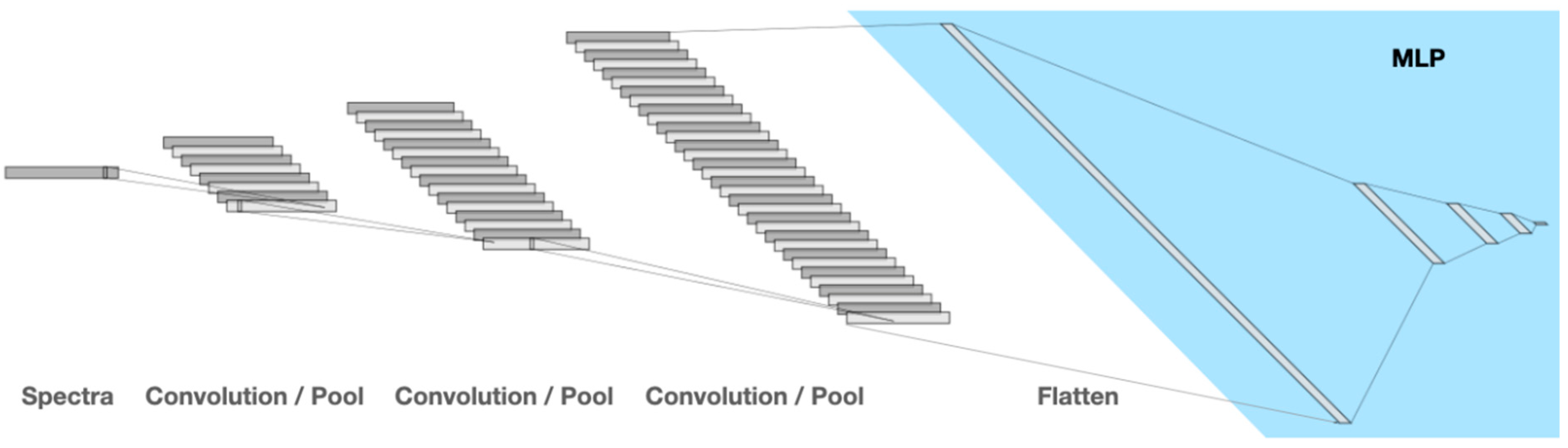
4.2. Convolutional Neural Networks
Author Contributions
Funding
Institutional Review Board Statement
Informed Consent Statement
Data Availability Statement
Conflicts of Interest
References
- REGULATION (EU) 2017/745 OF THE EUROPEAN PARLIAMENT AND OF THE COUNCIL of 5 April 2017 on medical devices, amending Directive 2001/83/EC, Regulation (EC) No 178/2002 and Regulation (EC) No 1223/2009 and repealing Council Directives 90/385/EEC and 93/42/EEC. Off. J. Eur. Union 2017, L117, 1–175.
- Ikeda, K.; Ichihara, K.; Hashiguchi, T.; Hidaka, Y.; Kang, D.; Maekawa, M.; Matsumoto, H.; Matsushita, K.; Okubo, S.; Tsuchiya, T.; et al. Evaluation of the short-term stability of specimens for clinical laboratory testing. Biopreserv. Biobank. 2015, 13, 135–143. [Google Scholar] [CrossRef] [PubMed]
- Toulon, P.; Metge, S.; Hangard, M.; Zwahlen, S.; Piaulenne, S.; Besson, V. Impact of different storage times at room temperature of unspun citrated blood samples on routine coagulation tests results. Results of a bicenter study and review of the literature. Int. J. Lab. Hematol. 2017, 39, 458–468. [Google Scholar] [CrossRef] [PubMed]
- van Geest-Daalderop, J.H.H.; Mulder, A.B.; Boonman-de Winter, L.J.M.; Hoekstra, M.M.C.L.; van den Besselaar, A.M.H.P. Preanalytical variables and off-site blood collection: Influences on the results of the prothrombin time/international normalized ratio test and implications for monitoring of oral anticoagulant therapy. Clin. Chem. 2005, 51, 561–568. [Google Scholar] [CrossRef]
- Carraro, P.; Plebani, M. Errors in a stat laboratory: Types and frequencies 10 years later. Clin. Chem. 2007, 53, 1338–1342. [Google Scholar] [CrossRef]
- Green, S.F. The cost of poor blood specimen quality and errors in preanalytical processes. Clin. Biochem. 2013, 46, 1175–1179. [Google Scholar] [CrossRef]
- Kang, H.J.; Jeon, S.Y.; Park, J.-S.; Yun, J.Y.; Kil, H.N.; Hong, W.K.; Lee, M.-H.; Kim, J.-W.; Jeon, J.-P.; Han, B.G. Identification of clinical biomarkers for pre-analytical quality control of blood samples. Biopreserv. Biobank. 2013, 11, 94–100. [Google Scholar] [CrossRef]
- Correia, N.A.; Batista, L.T.A.; Nascimento, R.J.M.; Cangussú, M.C.T.; Crugeira, P.J.L.; Soares, L.G.P.; Silveira, L.; Pinheiro, A.L.B. Detection of prostate cancer by Raman spectroscopy: A multivariate study on patients with normal and altered PSA values. J. Photochem. Photobiol. B 2020, 204, 111801. [Google Scholar] [CrossRef]
- Eberhardt, K.; Stiebing, C.; Matthäus, C.; Schmitt, M.; Popp, J. Advantages and limitations of Raman spectroscopy for molecular diagnostics: An update. Expert Rev. Mol. Diagn. 2015, 15, 773–787. [Google Scholar] [CrossRef]
- Wang, W.; Dong, R.-L.; Gu, D.; He, J.-A.; Yi, P.; Kong, S.-K.; Ho, H.-P.; Loo, J.F.-C.; Wang, W.; Wang, Q. Antibody-free rapid diagnosis of malaria in whole blood with surface-enhanced Raman Spectroscopy using Nanostructured Gold Substrate. Adv. Med. Sci. 2020, 65, 86–92. [Google Scholar] [CrossRef]
- Pahlow, S.; Meisel, S.; Cialla-May, D.; Weber, K.; Rösch, P.; Popp, J. Isolation and identification of bacteria by means of Raman spectroscopy. Adv. Drug Deliv. Rev. 2015, 89, 105–120. [Google Scholar] [CrossRef] [PubMed]
- Ho, C.-S.; Jean, N.; Hogan, C.A.; Blackmon, L.; Jeffrey, S.S.; Holodniy, M.; Banaei, N.; Saleh, A.A.E.; Ermon, S.; Dionne, J. Rapid identification of pathogenic bacteria using Raman spectroscopy and deep learning. Nat. Commun. 2019, 10, 4927. [Google Scholar] [CrossRef] [PubMed]
- Staritzbichler, R.; Hunold, P.; Estrela-Lopis, I.; Hildebrand, P.W.; Isermann, B.; Kaiser, T. Raman spectroscopy on blood serum samples of patients with end-stage liver disease. PLoS ONE 2021, 16, e0256045. [Google Scholar] [CrossRef] [PubMed]
- LeNail, A. NN-SVG: Publication-Ready Neural Network Architecture Schematics. J. Open Source Softw. 2019, 4, 747. [Google Scholar] [CrossRef]
- Hall, K.K.; Lyman, J.A. Updated review of blood culture contamination. Clin. Microbiol. Rev. 2006, 19, 788–802. [Google Scholar] [CrossRef]
- Valueva, M.V.; Nagornov, N.N.; Lyakhov, P.A.; Valuev, G.V.; Chervyakov, N.I. Application of the residue number system to reduce hardware costs of the convolutional neural network implementation. Math. Comput. Simul. 2020, 177, 232–243. [Google Scholar] [CrossRef]
- Collobert, R.; Weston, J. A unified architecture for natural language processing. In Proceedings of the 25th International Conference on Machine Learning-ICML ‘08, Helsinki, Finland, 5–9 July 2008; Cohen, W., McCallum, A., Roweis, S., Eds.; ACM Press: New York, NY, USA, 2008; pp. 160–167, ISBN 9781605582054. [Google Scholar]
- Tsantekidis, A.; Passalis, N.; Tefas, A.; Kanniainen, J.; Gabbouj, M.; Iosifidis, A. Forecasting Stock Prices from the Limit Order Book Using Convolutional Neural Networks. In Proceedings of the 2017 IEEE 19th Conference on Business Informatics (CBI), Thessaloniki, Greece, 24–27 July 2017; pp. 7–12, ISBN 978-1-5386-3035-8. [Google Scholar]
- Liu, Y.; Sung, K.; Yang, G.; Afshari Mirak, S.; Hosseiny, M.; Azadikhah, A.; Zhong, X.; Reiter, R.E.; Lee, Y.; Raman, S.S. Automatic Prostate Zonal Segmentation Using Fully Convolutional Network With Feature Pyramid Attention. IEEE Access 2019, 7, 163626–163632. [Google Scholar] [CrossRef]
- Wang, S.; Dai, C.; Mo, Y.; Angelini, E.; Guo, Y.; Bai, W. Automatic Brain Tumour Segmentation and Biophysics-Guided Survival Prediction. In Brainlesion: Glioma, Multiple Sclerosis, Stroke and Traumatic Brain Injuries; Crimi, A., Bakas, S., Eds.; Springer International Publishing: Cham, Switzerland, 2020; pp. 61–72. ISBN 978-3-030-46642-8. [Google Scholar]
- Roth, H.R.; Oda, H.; Zhou, X.; Shimizu, N.; Yang, Y.; Hayashi, Y.; Oda, M.; Fujiwara, M.; Misawa, K.; Mori, K. An application of cascaded 3D fully convolutional networks for medical image segmentation. Comput. Med. Imaging Graph. 2018, 66, 90–99. [Google Scholar] [CrossRef]
- Baldeon Calisto, M.; Lai-Yuen, S.K. AdaEn-Net: An ensemble of adaptive 2D-3D Fully Convolutional Networks for medical image segmentation. Neural Netw. 2020, 126, 76–94. [Google Scholar] [CrossRef]
- Zeng, Y.; Zhang, M.; Han, F.; Gong, Y.; Zhang, J. Spectrum Analysis and Convolutional Neural Network for Automatic Modulation Recognition. IEEE Wireless Commun. Lett. 2019, 8, 929–932. [Google Scholar] [CrossRef]
- Fukuhara, M.; Fujiwara, K.; Maruyama, Y.; Itoh, H. Feature visualization of Raman spectrum analysis with deep convolutional neural network. Anal. Chim. Acta 2019, 1087, 11–19. [Google Scholar] [CrossRef] [PubMed]
- Albelwi, S.; Mahmood, A. Automated Optimal Architecture of Deep Convolutional Neural Networks for Image Recognition. In Proceedings of the 15th IEEE International Conference on Machine Learning and Applications (ICMLA), Anaheim, CA, USA, 18–20 December 2016; pp. 53–60, ISBN 978-1-5090-6167-9. [Google Scholar]


| Training/Test Data/Number of Spectra | 80%/20%/1603 |
| Number of convolution layers | 3 |
| Kernel sizes | 3, 3, 3 |
| Number of descriptors | 8, 16, 32 |
| Maximum pooling sizes | 3, 3, 3 |
| Number of MLP hidden layers | 3 |
| Sizes of hidden layers | 256, 128, 64 |
| Optimizer | AdamW |
| Activation function | Leaky ReLU |
| Learning rate | 9 × 10⁻⁷ |
| Loss function | Cross entropy |
| Day | 0 | 1 | 2 | 3 | 4 | 5 | 6 | 7 |
|---|---|---|---|---|---|---|---|---|
| Number of Measured Samples | 330 | 330 | 106 | 294 | 230 | 38 | 144 | 155 |
| day 0 | sample was removed from freezer (−20 °C), thawed; 50 µL was measured and discarded | after measurement, stored at room temperature (22 °C) until next day |
| day 1 | sample (50 µL) was measured and discarded | after measurement, stored in refrigerator at 7 °C until the next day |
| days 2–6 | sample removed from refrigerator, 50 µL was measured and discarded | after measurement, stored in refrigerator at 7 °C until the next day |
| day 7 | sample removed from refrigerator, 50 µL was measured and discarded | after measurement, disposal of sample |
| Female | Male | Total | |
|---|---|---|---|
| Number of patients | 137 | 193 | 330 |
| Age (range) [years] | 54.7 (31–70) | 56.8 (21–77) | 55.8 (21–77) |
| Bilirubin (range) [µmol/L] | 70.9 (3.2–537.6) | 87.6 (3–911.2) | 80.7 (3–911.2) |
| Creatinine (range) [µmol/L] | 96.8 (29–333) | 131.4 (44–707) | 117.0 (29–707) |
| INR (range) | 1.5 (0.9–2.5) | 1.45 (0.9–3.3) | 1.47 (0.9–3.3) |
| MELD (range) | 16.2 (6–39) | 15.5 (6–40) | 15 (6–40) |
Disclaimer/Publisher’s Note: The statements, opinions and data contained in all publications are solely those of the individual author(s) and contributor(s) and not of MDPI and/or the editor(s). MDPI and/or the editor(s) disclaim responsibility for any injury to people or property resulting from any ideas, methods, instructions or products referred to in the content. |
© 2023 by the authors. Licensee MDPI, Basel, Switzerland. This article is an open access article distributed under the terms and conditions of the Creative Commons Attribution (CC BY) license (https://creativecommons.org/licenses/by/4.0/).
Share and Cite
Hunold, P.; Fischer, M.; Olthoff, C.; Hildebrand, P.W.; Kaiser, T.; Staritzbichler, R. Detecting Pre-Analytically Delayed Blood Samples for Laboratory Diagnostics Using Raman Spectroscopy. Int. J. Mol. Sci. 2023, 24, 7853. https://doi.org/10.3390/ijms24097853
Hunold P, Fischer M, Olthoff C, Hildebrand PW, Kaiser T, Staritzbichler R. Detecting Pre-Analytically Delayed Blood Samples for Laboratory Diagnostics Using Raman Spectroscopy. International Journal of Molecular Sciences. 2023; 24(9):7853. https://doi.org/10.3390/ijms24097853
Chicago/Turabian StyleHunold, Pascal, Markus Fischer, Carsten Olthoff, Peter W. Hildebrand, Thorsten Kaiser, and René Staritzbichler. 2023. "Detecting Pre-Analytically Delayed Blood Samples for Laboratory Diagnostics Using Raman Spectroscopy" International Journal of Molecular Sciences 24, no. 9: 7853. https://doi.org/10.3390/ijms24097853