
Machine Learning Models for the Identification of Prognostic and Predictive Cancer Biomarkers: A Systematic Review
 ,
,  ,
,  , , and
Abstract
:1. Introduction
- Diagnostic biomarkers predict the occurrence of an illness or classify people based on disease subtype. For example, individuals diagnosed with diffuse large B-cell lymphoma may be classified into subgroups using gene expression profiling of unique tumor cell signatures [6].
- Prognostic biomarkers provide information regarding a potential cancer outcome, with or without therapy [5].
- Predictive biomarkers indicate the likelihood of a patient’s response to a treatment plan and can be used to categorize patients as having a higher or lower chance of responding to a specific regimen, resulting in a gain in therapeutic precision [5].
- Monitoring biomarkers are evaluated frequently over time to identify disease incidence, incidence or recurrence, disease progression, or other clinically relevant changes. For example, CA 125 is used to assess disease activity or burden in patients with ovarian cancer before and after surgery [7].
- Safety biomarkers are evaluated prior to or following exposure to a therapeutic medication or environmental substance to determine the probability, frequency, and severity of toxicity as an adverse reaction. For example, serum creatinine in patients who are taking potentially nephrotoxic drugs is one of this biomarker type [8].
- Response biomarkers demonstrate the physiological reaction of a patient to a medicinal drug or environmental contaminant. Plasma microRNAs, for instance, are used as a response biomarker for Hodgkin lymphoma [9].
- Risk biomarkers indicate the likelihood that a person may develop an illness or health condition. They are particularly helpful for directing preventive actions in clinical practice. The BRCA1 and BRCA2 mutations, which evaluate the likelihood of breast carcinoma production, are two of the most recognized risk biomarkers, and BRCA carriers often undergo radical preventive measures to avoid the development of future cancers, such as elective mastectomy or salpingo-oophorectomy [7].
2. Methods
2.1. Evidence Acquisition
2.1.1. Aim
- RQ1: What machine learning models are currently being utilized to identify prognostic and predictive biomarkers?
- RQ2: What kinds of model validation techniques have been utilized during the construction of machine learning models to identify biomarkers?
- RQ3: What metrics have been utilized to evaluate the efficacy of the machine learning models in detecting the biomarkers?
- RQ4: What are the key cancer applications used to validate the existing machine learning models?
2.1.2. Search Strategy
2.1.3. Study Selection Criteria
- The study had to be published between 1 January 2017 and 1 January 2023.
- The study must be related to the use of machine learning models in the identification of prognostic and predictive biomarkers.
- The study must include only cancer disease biomarkers (any type).
- The study must have been published in a peer-reviewed journal.
- The article must have a full-text version, and the most comprehensive version was included, if applicable.
- The study was published before 1 January 2017 or after 1 January 2023.
- The study was published in an informal location or unknown source, or the paper was irrelevant to the domain of machine learning for identifying prognostic and predictive biomarkers.
- The study focused on biomarkers of non-cancer disease(s).
- The study was published in a language besides English or the publication had already been selected for the study.
- Reviews, systematic reviews, meta-analyses, and abstract publications were excluded.
2.2. Evidence Synthesis
3. Results
4. Application
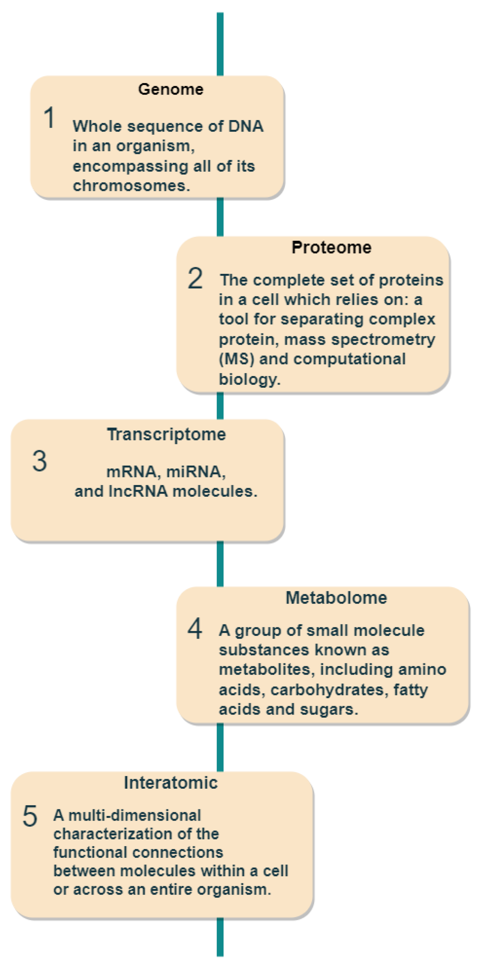
- Genome: medical genomics aims to detect genetic variations that correlate with illness, treatment efficacy, and patient prognosis [44].
- Proteome: detects changes in protein expression induced by a definite stimulus at a particular moment and identifies the configuration of protein networks at the cellular, organismal, or tissue level [45].
- Transcriptome: RNA serves as the intermediary among DNA and proteins, acting as the primary conduit for DNA-derived information [46]. The RNA-Seq method is used to analyze the transcripts or atomic dataset.
- Metabolome: Metabolomics is conducted at various levels of metabolites, and any relative imbalances or disruptions that are comparatively abnormal indicate the presence of illness [47].
- Interatomic: Protein-protein interactions are belonging to this type of omics data [48].
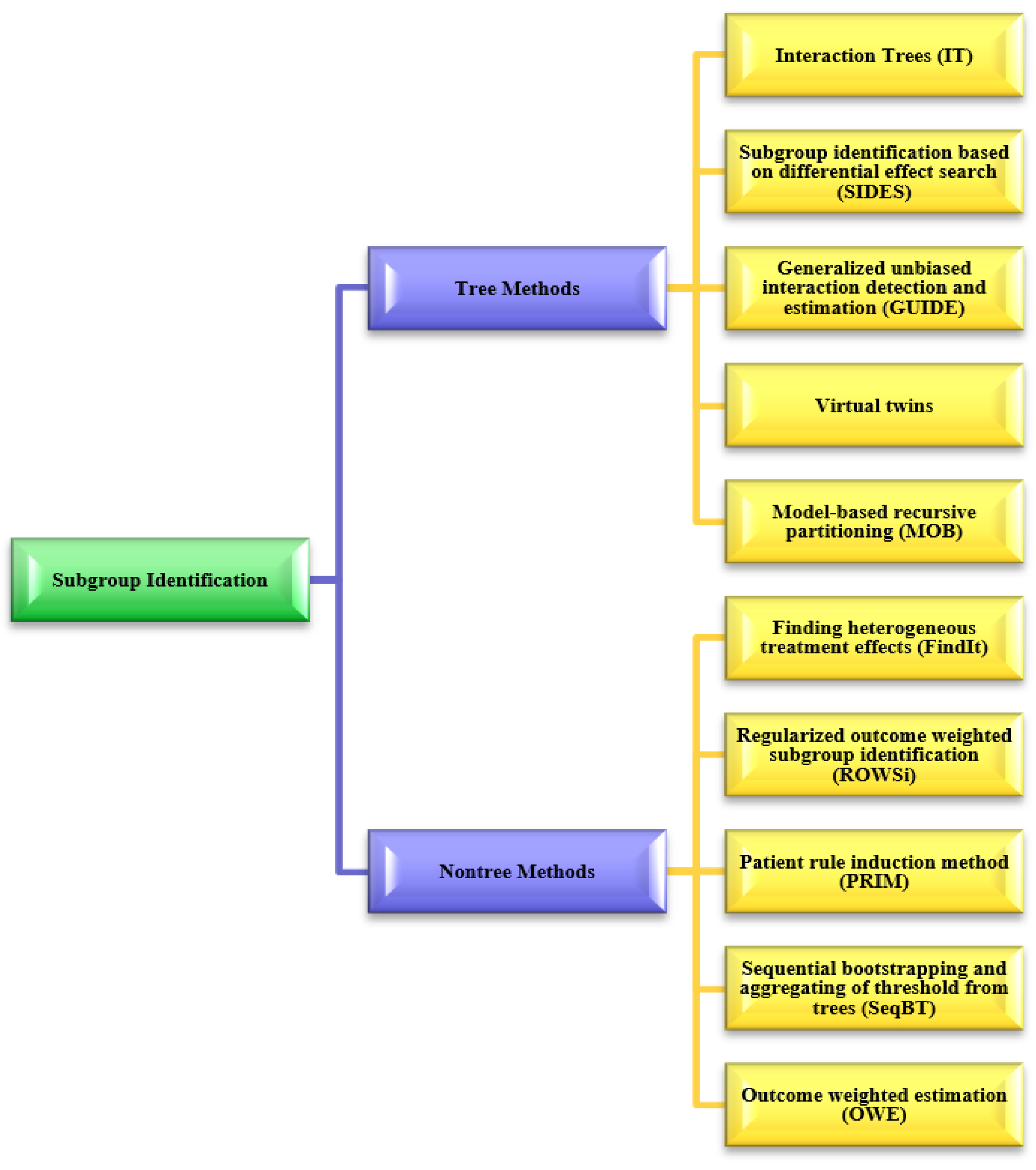
5. Subgroup Identification for Precision Medicine
6. Discussion
6.1. RQ1: What Machine Learning Models Are Currently Being Used to Identify Prognostic and Predictive Biomarkers?
6.2. RQ2: Which Types of Model Validation Have Been Employed in the Development of Machine Learning Models for Biomarker Identification?
6.3. RQ3: What Evaluation Measures Have Been Used to Assess the Performance of the Machine Learning Models in Identifying the Biomarkers?
- The hazard ratio (HR): A measure that compares the likelihood of an event occurring in a group receiving treatment to the likelihood of the same event happening in a group not receiving treatment, allowing researchers to determine if patients undergoing treatment experience an event faster (or slower) than those who are not [88].
- The concordance index (C-index): is widely used in survival analysis as a measure of discrimination [89] and is favored for its interpretability, as it is similar to classification accuracy and receiver operator characteristic area under the curve. Simply put, the C-index estimates the likelihood that, for a randomly selected pair of individuals, the predicted survival times are ordered in the same way as the actual survival times [90].
- The log-rank test: is a non-parametric statistical test used to compare the survival experiences between two groups and is commonly used in clinical trials to determine if one treatment leads to a longer survival time compared to another treatment [91]. Kaplan–Meier analysis and log-rank tests are usually used to evaluate the statistical significance between groups of patients [92].
- p-values are used to determine if an observed pattern is statistically significant (i.e., the p-value of a statistical test is low enough to reject the null hypothesis). The commonly accepted threshold for a low p-value is p < 0.05, which is roughly equivalent to the chance that the null hypothesis value (commonly assumed to be zero) falls within a 95% confidence interval [93].
6.4. RQ4: What Are the Key Cancer Applications Used to Validate the Existing Machine-Learning Models?
6.5. Challenges in Biomarker Discovery
6.6. Future Research Directions
- Developing feature selection approaches that overcome the limitations of existing approaches, e.g., swarm intelligence and meta-heuristic algorithms could help accurately identify prognostic and predictive biomarkers due to their robust performance in the feature selection field [103,104,105,106,107].
- Developing or improving non-linear models that integrate deep learning algorithms, such as DeepSurv [108], for better signature gene identification with prognostic and predictive biomarkers.
- Addressing the treatment effect that could be offered based on the biomarker’s identification, improving the current subgroup identification methods, and focusing more on the identification of predictive biomarkers.
- Including more independent or external data cohorts to conduct a comprehensive investigation into the progression, diagnosis, and treatment of cancer.
6.7. Limitations of This Systematic Review
7. Conclusions
Author Contributions
Funding
Institutional Review Board Statement
Informed Consent Statement
Data Availability Statement
Acknowledgments
Conflicts of Interest
References
- Chan, I.S.; Ginsburg, G.S. Personalized medicine: Progress and promise. Annu. Rev. Genom. Hum. Genet. 2011, 12, 217–244. [Google Scholar] [CrossRef]
- Lu, Y.; Zhou, J.; Xing, L.; Zhang, X. The optimal design of clinical trials with potential biomarker effects: A novel computational approach. Stat. Med. 2021, 40, 1752–1766. [Google Scholar] [CrossRef] [PubMed]
- Landeck, L.; Kneip, C.; Reischl, J.; Asadullah, K. Biomarkers and personalized medicine: Current status and further perspectives with special focus on dermatology. Exp. Dermatol. 2016, 25, 333–339. [Google Scholar] [CrossRef] [PubMed]
- Beckman, R.A.; Chen, C. Efficient, adaptive clinical validation of predictive biomarkers in cancer therapeutic development. Adv. Cancer Biomark. 2015, 867, 81–90. [Google Scholar]
- Ballman, K.V. Biomarker: Predictive or prognostic? J. Clin. Oncol. Off. J. Am. Soc. Clin. Oncol. 2015, 33, 3968–3971. [Google Scholar] [CrossRef]
- Khan, T. Introduction to Alzheimer’s disease biomarkers. In Biomarkers in Alzheimer’s Disease; Academic: New York, NY, USA, 2016; p. 13. [Google Scholar]
- Cagney, D.N.; Sul, J.; Huang, R.Y.; Ligon, K.L.; Wen, P.Y.; Alexander, B.M. The FDA NIH Biomarkers, EndpointS, and other Tools (BEST) resource in neuro-oncology. Neuro-oncology 2018, 20, 1162–1172. [Google Scholar] [CrossRef]
- Matheis, K.; Laurie, D.; Andriamandroso, C.; Arber, N.; Badimon, L.; Benain, X.; Bendjama, K.; Clavier, I.; Colman, P.; Firat, H. A generic operational strategy to qualify translational safety biomarkers. Drug Discov. Today 2011, 16, 600–608. [Google Scholar] [CrossRef]
- Jones, K.; Nourse, J.P.; Keane, C.; Bhatnagar, A.; Gandhi, M.K. Plasma MicroRNA Are Disease Response Biomarkers in Classical Hodgkin LymphomaPlasma miRNA Disease Response Biomarkers in cHL. Clin. Cancer Res. 2014, 20, 253–264. [Google Scholar] [CrossRef]
- Hong, L.; Aminu, M.; Li, S.; Lu, X.; Petranovic, M.; Saad, M.B.; Chen, P.; Qin, K.; Varghese, S.; Rinsurongkawong, W. Efficacy and clinicogenomic correlates of response to immune checkpoint inhibitors alone or with chemotherapy in non-small cell lung cancer. Nat. Commun. 2023, 14, 695. [Google Scholar] [CrossRef]
- Sechidis, K.; Papangelou, K.; Metcalfe, P.D.; Svensson, D.; Weatherall, J.; Brown, G. Distinguishing prognostic and predictive biomarkers: An information theoretic approach. Bioinformatics 2018, 34, 3365–3376. [Google Scholar] [CrossRef]
- Lipkovich, I.; Dmitrienko, A.; BD’Agostino, R., Sr. Tutorial in biostatistics: Data-driven subgroup identification and analysis in clinical trials. Stat. Med. 2017, 36, 136–196. [Google Scholar] [CrossRef] [PubMed]
- Moher, D.; Liberati, A.; Tetzlaff, J.; Altman, D.G.; The PRISMA Group. Preferred reporting items for systematic reviews and meta-analyses: The PRISMA statement. Ann. Intern. Med. 2009, 151, 264–269. [Google Scholar] [CrossRef] [PubMed]
- Cheong, J.-H.; Wang, S.C.; Park, S.; Porembka, M.R.; Christie, A.L.; Kim, H.; Kim, H.S.; Zhu, H.; Hyung, W.J.; Noh, S.H. Development and validation of a prognostic and predictive 32-gene signature for gastric cancer. Nat. Commun. 2022, 13, 774. [Google Scholar] [CrossRef] [PubMed]
- Lee, J.Y.; Lee, K.-s.; Seo, B.K.; Cho, K.R.; Woo, O.H.; Song, S.E.; Kim, E.-K.; Lee, H.Y.; Kim, J.S.; Cha, J. Radiomic machine learning for predicting prognostic biomarkers and molecular subtypes of breast cancer using tumor heterogeneity and angiogenesis properties on MRI. Eur. Radiol. 2022, 32, 650–660. [Google Scholar] [CrossRef] [PubMed]
- Lee, C.J.; Baek, B.; Cho, S.H.; Jang, T.Y.; Jeon, S.E.; Lee, S.; Lee, H.; Nam, J.S. Machine learning with in silico analysis markedly improves survival prediction modeling in colon cancer patients. Cancer Med. 2022, 12, 7603–7615. [Google Scholar] [CrossRef] [PubMed]
- Yen, R.; Grasedieck, S.; Wu, A.; Lin, H.; Su, J.; Rothe, K.; Nakamoto, H.; Forrest, D.L.; Eaves, C.J.; Jiang, X. Identification of key microRNAs as predictive biomarkers of Nilotinib response in chronic myeloid leukemia: A sub-analysis of the ENESTxtnd clinical trial. Leukemia 2022, 36, 2443–2452. [Google Scholar] [CrossRef]
- Patel, A.J.; Tan, T.-M.; Richter, A.G.; Naidu, B.; Blackburn, J.M.; Middleton, G.W. A highly predictive autoantibody-based biomarker panel for prognosis in early-stage NSCLC with potential therapeutic implications. Br. J. Cancer 2022, 126, 238–246. [Google Scholar] [CrossRef]
- Zhang, G.-Z.; Wu, Z.-L.; Li, C.-Y.; Ren, E.-H.; Yuan, W.-H.; Deng, Y.-J.; Xie, Q.-Q. Development of a machine learning-based autophagy-related lncRNA signature to improve prognosis prediction in osteosarcoma patients. Front. Mol. Biosci. 2021, 8, 615084. [Google Scholar] [CrossRef]
- Amiri Souri, E.; Chenoweth, A.; Cheung, A.; Karagiannis, S.N.; Tsoka, S. Cancer Grade Model: A multi-gene machine learning-based risk classification for improving prognosis in breast cancer. Br. J. Cancer 2021, 125, 748–758. [Google Scholar] [CrossRef]
- Xu, W.; Anwaier, A.; Ma, C.; Liu, W.; Tian, X.; Palihati, M.; Hu, X.; Qu, Y.; Zhang, H.; Ye, D. Multi-omics reveals novel prognostic implication of SRC protein expression in bladder cancer and its correlation with immunotherapy response. Ann. Med. 2021, 53, 596–610. [Google Scholar] [CrossRef]
- Taneja, I.; Damhorst, G.L.; Lopez-Espina, C.; Zhao, S.D.; Zhu, R.; Khan, S.; White, K.; Kumar, J.; Vincent, A.; Yeh, L. Diagnostic and prognostic capabilities of a biomarker and EMR-based machine learning algorithm for sepsis. Clin. Transl. Sci. 2021, 14, 1578–1589. [Google Scholar] [CrossRef] [PubMed]
- Arora, C.; Kaur, D.; Naorem, L.D.; Raghava, G.P. Prognostic biomarkers for predicting papillary thyroid carcinoma patients at high risk using nine genes of apoptotic pathway. PLoS ONE 2021, 16, e0259534. [Google Scholar] [CrossRef]
- Wang, T.-H.; Lee, C.-Y.; Lee, T.-Y.; Huang, H.-D.; Hsu, J.B.-K.; Chang, T.-H. Biomarker identification through multiomics data analysis of prostate cancer prognostication using a deep learning model and similarity network fusion. Cancers 2021, 13, 2528. [Google Scholar] [CrossRef] [PubMed]
- Moore, M.R.; Friesner, I.D.; Rizk, E.M.; Fullerton, B.T.; Mondal, M.; Trager, M.H.; Mendelson, K.; Chikeka, I.; Kurc, T.; Gupta, R. Automated digital TIL analysis (ADTA) adds prognostic value to standard assessment of depth and ulceration in primary melanoma. Sci. Rep. 2021, 11, 2809. [Google Scholar] [CrossRef] [PubMed]
- Liu, Z.; Mi, M.; Li, X.; Zheng, X.; Wu, G.; Zhang, L. A lncRNA prognostic signature associated with immune infiltration and tumour mutation burden in breast cancer. J. Cell. Mol. Med. 2020, 24, 12444–12456. [Google Scholar] [CrossRef] [PubMed]
- Zhang, Z.; Pan, Q.; Ge, H.; Xing, L.; Hong, Y.; Chen, P. Deep learning-based clustering robustly identified two classes of sepsis with both prognostic and predictive values. EBioMedicine 2020, 62, 103081. [Google Scholar] [CrossRef]
- Skrede, O.-J.; De Raedt, S.; Kleppe, A.; Hveem, T.S.; Liestøl, K.; Maddison, J.; Askautrud, H.A.; Pradhan, M.; Nesheim, J.A.; Albregtsen, F. Deep learning for prediction of colorectal cancer outcome: A discovery and validation study. Lancet 2020, 395, 350–360. [Google Scholar] [CrossRef]
- Cai, Q.; He, B.; Zhang, P.; Zhao, Z.; Peng, X.; Zhang, Y.; Xie, H.; Wang, X. Exploration of predictive and prognostic alternative splicing signatures in lung adenocarcinoma using machine learning methods. J. Transl. Med. 2020, 18, 463. [Google Scholar] [CrossRef]
- Ma, B.; Geng, Y.; Meng, F.; Yan, G.; Song, F. Identification of a sixteen-gene prognostic biomarker for lung adenocarcinoma using a machine learning method. J. Cancer 2020, 11, 1288. [Google Scholar] [CrossRef]
- Fortino, V.; Scala, G.; Greco, D. Feature set optimization in biomarker discovery from genome-scale data. Bioinformatics 2020, 36, 3393–3400. [Google Scholar] [CrossRef]
- Tang, W.; Cao, Y.; Ma, X. Novel prognostic prediction model constructed through machine learning on the basis of methylation-driven genes in kidney renal clear cell carcinoma. Biosci. Rep. 2020, 40, BSR20201604. [Google Scholar] [CrossRef] [PubMed]
- Wang, Y.; Zhang, M.; Hu, X.; Qin, W.; Wu, H.; Wei, M. Colon cancer-specific diagnostic and prognostic biomarkers based on genome-wide abnormal DNA methylation. Aging 2020, 12, 22626. [Google Scholar] [CrossRef]
- Wang, S.; Liu, Z.; Rong, Y.; Zhou, B.; Bai, Y.; Wei, W.; Wang, M.; Guo, Y.; Tian, J. Deep learning provides a new computed tomography-based prognostic biomarker for recurrence prediction in high-grade serous ovarian cancer. Radiother. Oncol. 2019, 132, 171–177. [Google Scholar] [CrossRef] [PubMed]
- Kawakami, E.; Tabata, J.; Yanaihara, N.; Ishikawa, T.; Koseki, K.; Iida, Y.; Saito, M.; Komazaki, H.; Shapiro, J.S.; Goto, C. Application of Artificial Intelligence for Preoperative Diagnostic and Prognostic Prediction in Epithelial Ovarian Cancer Based on Blood BiomarkersArtificial Intelligence in Epithelial Ovarian Cancer. Clin. Cancer Res. 2019, 25, 3006–3015. [Google Scholar] [CrossRef] [PubMed]
- Park, E.K.; Lee, K.-s.; Seo, B.K.; Cho, K.R.; Woo, O.H.; Son, G.S.; Lee, H.Y.; Chang, Y.W. Machine learning approaches to radiogenomics of breast cancer using low-dose perfusion computed tomography: Predicting prognostic biomarkers and molecular subtypes. Sci. Rep. 2019, 9, 17847. [Google Scholar] [CrossRef] [PubMed]
- Liu, F.; Xing, L.; Zhang, X.; Zhang, X. A four-pseudogene classifier identified by machine learning serves as a novel prognostic marker for survival of osteosarcoma. Genes 2019, 10, 414. [Google Scholar] [CrossRef] [PubMed]
- Cheng, P. A prognostic 3-long noncoding RNA signature for patients with gastric cancer. J. Cell. Biochem. 2018, 119, 9261–9269. [Google Scholar] [CrossRef]
- Harder, N.; Athelogou, M.; Hessel, H.; Brieu, N.; Yigitsoy, M.; Zimmermann, J.; Baatz, M.; Buchner, A.; Stief, C.G.; Kirchner, T. Tissue Phenomics for prognostic biomarker discovery in low-and intermediate-risk prostate cancer. Sci. Rep. 2018, 8, 4470. [Google Scholar] [CrossRef]
- Choi, J.; Oh, I.; Seo, S.; Ahn, J. G2Vec: Distributed gene representations for identification of cancer prognostic genes. Sci. Rep. 2018, 8, 13729. [Google Scholar] [CrossRef]
- Kim, M.; Oh, I.; Ahn, J. An improved method for prediction of cancer prognosis by network learning. Genes 2018, 9, 478. [Google Scholar] [CrossRef]
- Huang, F.; Conley, A.; You, S.; Ma, Z.; Klimov, S.; Ohe, C.; Yuan, X.; Amin, M.B.; Figlin, R.; Gertych, A. A novel machine learning approach reveals latent vascular phenotypes predictive of renal cancer outcome. Sci. Rep. 2017, 7, 13190. [Google Scholar]
- Marquardt, J.U.; Galle, P.R.; Teufel, A. Molecular diagnosis and therapy of hepatocellular carcinoma (HCC): An emerging field for advanced technologies. J. Hepatol. 2012, 56, 267–275. [Google Scholar] [CrossRef] [PubMed]
- Bravo-Merodio, L.; Williams, J.A.; Gkoutos, G.V.; Acharjee, A. -Omics biomarker identification pipeline for translational medicine. J. Transl. Med. 2019, 17, 155. [Google Scholar] [CrossRef] [PubMed]
- Husi, H.; Albalat, A. Chapter 9—Proteomics. In Handbook of Pharmacogenomics and Stratified Medicine; Padmanabhan, S., Ed.; Academic Press: San Diego, CA, USA, 2014; pp. 147–179. [Google Scholar] [CrossRef]
- Kim, M.; Tagkopoulos, I. Data integration and predictive modeling methods for multi-omics datasets. Mol. Omics 2018, 14, 8–25. [Google Scholar] [CrossRef] [PubMed]
- Hasin, Y.; Seldin, M.; Lusis, A. Multi-omics approaches to disease. Genome Biol. 2017, 18, 83. [Google Scholar] [CrossRef] [PubMed]
- Cortese-Krott, M.M.; Santolini, J.; Wootton, S.A.; Jackson, A.A.; Feelisch, M. The reactive species interactome. In Oxidative Stress; Elsevier: Amsterdam, The Netherlands, 2020; pp. 51–64. [Google Scholar]
- König, I.R.; Fuchs, O.; Hansen, G.; von Mutius, E.; Kopp, M.V. What is precision medicine? Eur. Respir. J. 2017, 50, 1700391. [Google Scholar] [CrossRef]
- Chen, J.J.; Lu, T.-P.; Chen, Y.-C.; Lin, W.-J. Predictive biomarkers for treatment selection: Statistical considerations. Biomark. Med. 2015, 9, 1121–1135. [Google Scholar] [CrossRef]
- Loh, W.Y.; Cao, L.; Zhou, P. Subgroup identification for precision medicine: A comparative review of 13 methods. Wiley Interdiscip. Rev. Data Min. Knowl. Discov. 2019, 9, e1326. [Google Scholar] [CrossRef]
- Su, X.; Tsai, C.-L.; Wang, H.; Nickerson, D.M.; Li, B. Subgroup analysis via recursive partitioning. J. Mach. Learn. Res. 2009, 10, 141–158. [Google Scholar] [CrossRef]
- Su, X.; Zhou, T.; Yan, X.; Fan, J.; Yang, S. Interaction trees with censored survival data. Int. J. Biostat. 2008, 4, 2. [Google Scholar] [CrossRef]
- Lipkovich, I.; Dmitrienko, A.; Denne, J.; Enas, G. Subgroup identification based on differential effect search—A recursive partitioning method for establishing response to treatment in patient subpopulations. Stat. Med. 2011, 30, 2601–2621. [Google Scholar] [CrossRef] [PubMed]
- Foster, J.C.; Taylor, J.M.; Ruberg, S.J. Subgroup identification from randomized clinical trial data. Stat. Med. 2011, 30, 2867–2880. [Google Scholar] [CrossRef] [PubMed]
- Loh, W.Y.; Zhou, P. The GUIDE approach to subgroup identification. In Design and Analysis of Subgroups with Biopharmaceutical Applications; Springer: Cham, Switzerland, 2020; pp. 147–165. [Google Scholar] [CrossRef]
- Loh, W.Y. Regression tress with unbiased variable selection and interaction detection. Stat. Sin. 2002, 12, 361–386. [Google Scholar]
- Loh, W.Y. Improving the precision of classification trees. Ann. Appl. Stat. 2009, 3, 1710–1737. [Google Scholar] [CrossRef]
- Seibold, H.; Zeileis, A.; Hothorn, T. Model-based recursive partitioning for subgroup analyses. Int. J. Biostat. 2016, 12, 45–63. [Google Scholar] [CrossRef] [PubMed]
- Seibold, H.; Zeileis, A.; Hothorn, T. Individual treatment effect prediction for amyotrophic lateral sclerosis patients. Stat. Methods Med. Res. 2018, 27, 3104–3125. [Google Scholar] [CrossRef]
- Imai, K.; Ratkovic, M. Estimating treatment effect heterogeneity in randomized program evaluation. Ann. Appl. Stat. 2013, 7, 443–470. [Google Scholar] [CrossRef]
- Xu, Y.; Yu, M.; Zhao, Y.Q.; Li, Q.; Wang, S.; Shao, J. Regularized outcome weighted subgroup identification for differential treatment effects. Biometrics 2015, 71, 645–653. [Google Scholar] [CrossRef]
- Chen, G.; Zhong, H.; Belousov, A.; Devanarayan, V. A PRIM approach to predictive-signature development for patient stratification. Stat. Med. 2015, 34, 317–342. [Google Scholar] [CrossRef]
- Huang, X.; Sun, Y.; Trow, P.; Chatterjee, S.; Chakravartty, A.; Tian, L.; Devanarayan, V. Patient subgroup identification for clinical drug development. Stat. Med. 2017, 36, 1414–1428. [Google Scholar] [CrossRef]
- Chen, S.; Tian, L.; Cai, T.; Yu, M. A general statistical framework for subgroup identification and comparative treatment scoring. Biometrics 2017, 73, 1199–1209. [Google Scholar] [CrossRef] [PubMed]
- Härdle, W.K.; Simar, L.; Härdle, W.K.; Simar, L. Canonical correlation analysis. In Applied Multivariate Statistical Analysis; Springer: Berlin/Heidelberg, Germany, 2015; pp. 443–454. [Google Scholar]
- Xanthopoulos, P.; Pardalos, P.M.; Trafalis, T.B.; Xanthopoulos, P.; Pardalos, P.M.; Trafalis, T.B. Linear discriminant analysis. In Robust Data Mining; Springer: New York, NY, USA, 2013; pp. 27–33. [Google Scholar]
- Roweis, S.T.; Saul, L.K. Nonlinear dimensionality reduction by locally linear embedding. Science 2000, 290, 2323–2326. [Google Scholar] [CrossRef] [PubMed]
- Twining, C.J.; Taylor, C.J. The use of kernel principal component analysis to model data distributions. Pattern Recognit. 2003, 36, 217–227. [Google Scholar] [CrossRef]
- Belkina, A.C.; Ciccolella, C.O.; Anno, R.; Halpert, R.; Spidlen, J.; Snyder-Cappione, J.E. Automated optimized parameters for T-distributed stochastic neighbor embedding improve visualization and analysis of large datasets. Nat. Commun. 2019, 10, 5415. [Google Scholar] [CrossRef] [PubMed]
- Van der Maaten, L.; Hinton, G. Visualizing data using t-SNE. J. Mach. Learn. Res. 2008, 9, 2579–2605. [Google Scholar]
- Al-Tashi, Q.; Mirjalili, S.; Wu, J.; Abdulkadir, S.J.; Shami, T.M.; Khodadadi, N.; Alqushaibi, A. Moth-Flame Optimization Algorithm for Feature Selection: A Review and Future Trends. In Handbook of Moth-Flame Optimization Algorithm; CRC Press: Boca Raton, FL, USA, 2022; pp. 11–34. [Google Scholar]
- Al-Tashi, Q.; Md Rais, H.; Abdulkadir, S.J.; Mirjalili, S.; Alhussian, H. A review of grey wolf optimizer-based feature selection methods for classification. In Evolutionary Machine Learning Techniques. Algorithms for Intelligent Systems; Springer: Singapore, 2020; pp. 273–286. [Google Scholar]
- Lazar, C.; Taminau, J.; Meganck, S.; Steenhoff, D.; Coletta, A.; Molter, C.; de Schaetzen, V.; Duque, R.; Bersini, H.; Nowe, A. A survey on filter techniques for feature selection in gene expression microarray analysis. IEEE/ACM Trans. Comput. Biol. Bioinform. 2012, 9, 1106–1119. [Google Scholar] [CrossRef]
- Al-Tashi, Q.; Kadir, S.J.A.; Rais, H.M.; Mirjalili, S.; Alhussian, H. Binary optimization using hybrid grey wolf optimization for feature selection. IEEE Access 2019, 7, 39496–39508. [Google Scholar] [CrossRef]
- El Aboudi, N.; Benhlima, L. Review on wrapper feature selection approaches. In Proceedings of the 2016 International Conference on Engineering & MIS (ICEMIS), Agadir, Morocco, 22–24 September 2016; pp. 1–5. [Google Scholar]
- Al-Tashi, Q.; Abdulkadir, S.J.; Rais, H.M.; Mirjalili, S.; Alhussian, H.; Ragab, M.G.; Alqushaibi, A. Binary multi-objective grey wolf optimizer for feature selection in classification. IEEE Access 2020, 8, 106247–106263. [Google Scholar] [CrossRef]
- Al-Tashi, Q.; Rais, H.; Jadid, S. Feature selection method based on grey wolf optimization for coronary artery disease classification. In Proceedings of the Recent Trends in Data Science and Soft Computing: Proceedings of the 3rd International Conference of Reliable Information and Communication Technology (IRICT 2018), Kuala Lumpur, Malaysia, 23–24 July 2018; pp. 257–266. [Google Scholar]
- Spooner, A.; Chen, E.; Sowmya, A.; Sachdev, P.; Kochan, N.A.; Trollor, J.; Brodaty, H. A comparison of machine learning methods for survival analysis of high-dimensional clinical data for dementia prediction. Sci. Rep. 2020, 10, 20410. [Google Scholar] [CrossRef]
- Lao, J.; Chen, Y.; Li, Z.-C.; Li, Q.; Zhang, J.; Liu, J.; Zhai, G. A deep learning-based radiomics model for prediction of survival in glioblastoma multiforme. Sci. Rep. 2017, 7, 10353. [Google Scholar] [CrossRef]
- Dhillon, A.; Singh, A. Machine learning in healthcare data analysis: A survey. J. Biol. Today’s World 2019, 8, 1–10. [Google Scholar]
- Rashidi, H.H.; Tran, N.; Albahra, S.; Dang, L.T. Machine learning in health care and laboratory medicine: General overview of supervised learning and Auto-ML. Int. J. Lab. Hematol. 2021, 43, 15–22. [Google Scholar] [CrossRef] [PubMed]
- Hastie, T.; Tibshirani, R.; Friedman, J.; Hastie, T.; Tibshirani, R.; Friedman, J. Overview of supervised learning. Elem. Stat. Learn. Data Min. Inference Predict. 2009, 9–41. [Google Scholar] [CrossRef]
- Lewis, R.J. An introduction to classification and regression tree (CART) analysis. In Proceedings of the Annual Meeting of the Society for Academic Emergency Medicine in San Francisco, California, San Francisco, CA, USA, 22–25 May 2000. [Google Scholar]
- Barlow, H.B. Unsupervised learning. Neural Comput. 1989, 1, 295–311. [Google Scholar] [CrossRef]
- Kakarla, R.; Krishnan, S.; Alla, S.; Kakarla, R.; Krishnan, S.; Alla, S. Model Evaluation. In Applied Data Science Using PySpark; Apress: Berkeley, CA, USA, 2021; pp. 205–249. [Google Scholar]
- Montesinos López, O.A.; Montesinos López, A.; Crossa, J. Overfitting, Model Tuning, and Evaluation of Prediction Performance. In Multivariate Statistical Machine Learning Methods for Genomic Prediction; Springer: Berlin/Heidelberg, Germany, 2022; pp. 109–139. [Google Scholar]
- Spruance, S.L.; Reid, J.E.; Grace, M.; Samore, M. Hazard ratio in clinical trials. Antimicrob. Agents Chemother. 2004, 48, 2787–2792. [Google Scholar] [CrossRef] [PubMed]
- Longato, E.; Vettoretti, M.; Di Camillo, B. A practical perspective on the concordance index for the evaluation and selection of prognostic time-to-event models. J. Biomed. Inform. 2020, 108, 103496. [Google Scholar] [CrossRef]
- Brentnall, A.R.; Cuzick, J. Use of the concordance index for predictors of censored survival data. Stat. Methods Med. Res. 2018, 27, 2359–2373. [Google Scholar] [CrossRef]
- Bland, J.M.; Altman, D.G. The logrank test. BMJ 2004, 328, 1073. [Google Scholar] [CrossRef]
- Kleinbaum, D.G.; Klein, M.; Kleinbaum, D.G.; Klein, M. Kaplan-Meier survival curves and the log-rank test. In Survival Analysis. Statistics for Biology and Health; Springer: New York, NY, USA, 2012; pp. 55–96. [Google Scholar]
- Gardner, M.J.; Altman, D.G. Confidence intervals rather than P values: Estimation rather than hypothesis testing. Br. Med. J. 1986, 292, 746–750. [Google Scholar] [CrossRef]
- Jiao, Y.; Du, P. Performance measures in evaluating machine learning based bioinformatics predictors for classifications. Quant. Biol. 2016, 4, 320–330. [Google Scholar] [CrossRef]
- Hicks, S.A.; Strümke, I.; Thambawita, V.; Hammou, M.; Riegler, M.A.; Halvorsen, P.; Parasa, S. On evaluation metrics for medical applications of artificial intelligence. Sci. Rep. 2022, 12, 5979. [Google Scholar] [CrossRef] [PubMed]
- Handelman, G.S.; Kok, H.K.; Chandra, R.V.; Razavi, A.H.; Huang, S.; Brooks, M.; Lee, M.J.; Asadi, H. Peering into the black box of artificial intelligence: Evaluation metrics of machine learning methods. Am. J. Roentgenol. 2019, 212, 38–43. [Google Scholar] [CrossRef] [PubMed]
- Alba, A.C.; Agoritsas, T.; Walsh, M.; Hanna, S.; Iorio, A.; Devereaux, P.; McGinn, T.; Guyatt, G. Discrimination and calibration of clinical prediction models: Users’ guides to the medical literature. JAMA 2017, 318, 1377–1384. [Google Scholar] [CrossRef]
- Chen, P.-H.C.; Liu, Y.; Peng, L. How to develop machine learning models for healthcare. Nat. Mater. 2019, 18, 410–414. [Google Scholar] [CrossRef]
- Aminu, M.; Yadav, D.; Hong, L.; Young, E.; Edelkamp Jr, P.; Saad, M.; Salehjahromi, M.; Chen, P.; Sujit, S.J.; Chen, M.M. Habitat Imaging Biomarkers for Diagnosis and Prognosis in Cancer Patients Infected with COVID-19. Cancers 2022, 15, 275. [Google Scholar] [CrossRef] [PubMed]
- Wu, J.; Mayer, A.T.; Li, R. Integrated imaging and molecular analysis to decipher tumor microenvironment in the era of immunotherapy. In Seminars in Cancer Biology; Academic Press: New York, NY, USA, 2022; pp. 310–328. [Google Scholar]
- Chen, M.M.; Terzic, A.; Becker, A.S.; Johnson, J.M.; Wu, C.C.; Wintermark, M.; Wald, C.; Wu, J. Artificial intelligence in oncologic imaging. Eur. J. Radiol. Open 2022, 9, 100441. [Google Scholar] [CrossRef]
- Wu, J.; Li, C.; Gensheimer, M.; Padda, S.; Kato, F.; Shirato, H.; Wei, Y.; Schönlieb, C.-B.; Price, S.J.; Jaffray, D. Radiological tumour classification across imaging modality and histology. Nat. Mach. Intell. 2021, 3, 787–798. [Google Scholar] [CrossRef]
- Al-Tashi, Q.; Abdulkadir, S.J.; Rais, H.M.; Mirjalili, S.; Alhussian, H. Approaches to Multi-Objective Feature Selection: A Systematic Literature Review. IEEE Access 2020, 8, 125076–125096. [Google Scholar] [CrossRef]
- Al-Wajih, R.; Abdulkadir, S.J.; Aziz, N.; Al-Tashi, Q.; Talpur, N. Hybrid binary grey wolf with Harris hawks optimizer for feature selection. IEEE Access 2021, 9, 31662–31677. [Google Scholar] [CrossRef]
- Alwajih, R.; Abdulkadir, S.J.; Al Hussian, H.; Aziz, N.; Al-Tashi, Q.; Mirjalili, S.; Alqushaibi, A. Hybrid binary whale with harris hawks for feature selection. Neural Comput. Appl. 2022, 34, 19377–19395. [Google Scholar] [CrossRef]
- Shami, T.M.; El-Saleh, A.A.; Alswaitti, M.; Al-Tashi, Q.; Summakieh, M.A.; Mirjalili, S. Particle swarm optimization: A comprehensive survey. IEEE Access 2022, 10, 10031–10061. [Google Scholar] [CrossRef]
- Al-Tashi, Q.; Akhir, E.A.P.; Abdulkadir, S.J.; Mirjalili, S.; Shami, T.M.; Alhusssian, H.; Alqushaibi, A.; Alwadain, A.; Balogun, A.O.; Al-Zidi, N. Classification of reservoir recovery factor for oil and gas reservoirs: A multi-objective feature selection approach. J. Mar. Sci. Eng. 2021, 9, 888. [Google Scholar] [CrossRef]
- Katzman, J.L.; Shaham, U.; Cloninger, A.; Bates, J.; Jiang, T.; Kluger, Y. DeepSurv: Personalized treatment recommender system using a Cox proportional hazards deep neural network. BMC Med. Res. Methodol. 2018, 18, 24. [Google Scholar] [CrossRef] [PubMed]


| Refer | Year | Publisher | Machine Learning Methodology | Prognostic | Predictive | Measures | Validation | Results | Findings | Source Code |
|---|---|---|---|---|---|---|---|---|---|---|
| [14] | 2022 | Nature | An algorithm called (NTriPath) that utilizes machine learning was employed to discover a signature for gastric cancer. Unsupervised consensus clustering utilizing non-negative matrix factorization (NMF) was used to identify molecular subtypes that are prognostic for survival. Support vector machine (SVM) with linear kernel classifier was used to produce a risk score and to evaluate the effectiveness of NMF subgroups. Multivariable Cox proportional hazard analyses of overall survival were used within each genetic subgroup. Kaplan–Meier survival analysis was used to plot overall survival. | Yes | Yes | Hazard ratio (HR), p-value, risk score, log-rank, and area under the curve (AUC) | leave-one-out cross-validation and three independent test sets. | Using NTriPath, a gastric-cancer specific 32-gene signature was identified, and using NMF, 4 prognostic molecular subtypes were identified. The mean AUC for the classification was 0.981. | The 32-gene markers that were identified projected both overall survival (i.e., prognostic biomarkers) and response to treatments (i.e., predictive biomarkers). One group of patients obtained improved survival associated with adjuvant fluorouracil and platinum-based chemotherapy, and the other group had a worse response. The response to immune checkpoint inhibitors was linked to molecular classification. | NTriPath |
| [15] | 2022 | Springer | Perfusion and texture analyses were performed, and 160 parameters were extracted. First, a Mann–Whitney U test or t test was used to distinguish magnetic resonance imaging (MRI) parameters between pathologic biomarker groups. Second, a Kruskal–Wallis test and analysis of variance were used to compare MRI features among the four molecular subtypes. A post-hoc analysis was used to find different subgroups in case there were significant differences among subtypes in the above tests. Finally, five machine algorithms—logistic regression, decision tree, Naïve-Bayes (NB), random forest (RF), and artificial neural network (ANN)—were used to predict prognostic biomarkers and molecular subtypes. | Yes | No | AUC and p-value | Train-test split | Texture parameters were related with 6 parameters (p < 0.002). Perfusion parameters were associated with 4 parameters (p < 0.003). An RF model that combined texture and perfusion parameters produced an AUC of 0.75, which was the largest. | Integrating a radiomic model that incorporates angiogenesis characteristics and tumor heterogeneity holds promise in predicting prognostic factors for breast cancer. However, no treatment selection or predictive factors were identified in this study. | N/A |
| [16] | 2022 | Wiley | Machine learning analysis (logistic regression and autoencoder-based logistic regression) was used to screen pathogenic survival-related driver genes. Patient prognosis was analyzed by integrating copy number variation and gene expression data, and in silico analysis was presented to clinically assess data from the machine learning analysis. | Yes | No | AUC, F1 score, precision, and sensitivity | Five-fold cross-validation. | Three genes were identified as survival-related genes by machine learning and in silico experimental analysis. | The survival prediction approach provided information on patients and developing a therapeutic strategy for patients with colorectal cancer. No predictive biomarkers were reported. | N/A |
| [17] | 2022 | Nature | RF and NB machine-learning-based algorithms were used to identify important microRNAs as biomarkers for predicting the response of Nilotinib in chronic myeloid leukemia. | No | Yes | HR and receiver operator characteristics (ROC) | Ten-fold cross-validation | The combination of miR-145 and miR708 was an excellent predictor of nilotinib response in treatment-naive individuals, whereas miR-150 and miR-185 were significant classifiers at 1 month and 3 months after nilotinib therapy. | This study demonstrated that the integration of NL-CFC output into these panels enhanced their predictive ability. Therefore, this innovative predictive model may be adapted into a clinical prognostic tool. | N/A |
| [18] | 2022 | Nature | The authors attempted to predict an autoantibody-based biomarker panel for lung cancer using recursive-feature elimination with RF modelling and used least absolute shrinkage and selector operation (LASSO) regression with repeated 10-fold cross-validation. | No | Yes | AUC, sensitivity, specificity, ROC, and p-value | Ten-fold cross-validation | Strong expressers of an autoantibody-based biomarker profile had noticeably poor survivability, with an overall 5-year survival rate of 7.6%. | A profile of 13 predictive biomarkers outperformed the autoantibody biomarkers approaches adopted in solid malignancies for predicting survival in post-operative early-stage lung cancer. | N/A |
| [19] | 2021 | Frontiers | Univariate and multivariate Cox regression analyses were applied to evaluate the prognostic value of the autophagy-related long non-coding RNA (lncRNA) signature and to validate the association between the signature and survival of osteosarcoma patients in an independent cohort. | Yes | No | AUC, HR, z value, and p-value | Training and independent validation | Sixty-nine autophagy-related lncRNAs were identified, of which thirteen were significant predictors of the overall survival of patients with osteosarcoma. | Thirteen autophagy-related lncRNA prognostic biomarkers were identified in patients with osteosarcoma. No treatment selection had been performed. | N/A |
| [20] | 2021 | Nature | Gradient-boosted trees trained on histological grade 1 and grade 3 data. Several techniques were applied, including the detection of outliers using K-nearest neighbor, balancing the imbalanced dataset using the synthetic minority over-sampling technique, finding the best set of hyperparameters through a grid search on the training set samples and measuring the average performance across all cross-validation sets using the gain metric. To determine the most important features for classification, Shapley additive explanations was used. Finally, a principal component analysis was used. | Yes | No | Accuracy, gain, and Shapley additive explanations metrics | Ten-fold cross-validation | The identification of a 70-gene signature for determining clinical risk was demonstrated to be 90% accurate when used to evaluate samples with a known histological grade. | This model can classify high- and low-risk groups, without using clinical data, such as tumor size, tumor stage, or breast cancer subgroup. However, no experiments identified the responses to a specific treatment. | N/A |
| [21] | 2021 | Taylor & Francis | In this study, a multivariate analysis was employed to find the most significant prognostic proteins and calculate a risk score based on the expression of these proteins and the patients’ survival rate. Patients were divided into two groups: high risk or low risk, based on the median risk score. The correlation between the patient’s prognosis and the risk score was verified using survival curves and scatter diagrams. A heat map was created to visualize the expression of each candidate protein in the two groups. Univariate and multivariate Cox regression analyses were performed to determine the independent prognostic factors, which were used to build the IPRPs model. A cut-off value of 0.4 was used for the Pearson correlation analysis to determine the proteins associated with the IPRPs model. Results were considered significant if the p-value was less than 0.05. | Yes | Yes | AUC, log-rank test, and p-value | A validation cohort of 81 patients was used. | The prognosis-related protein model achieved diagnostic accuracy and had consistent predictive ability (AUC = 0.714). The results indicated that baseline SRC expression levels correlated with improved survival outcomes but predicted a worse response to immunotherapy. | This study highlighted the significance of the biomarker SRC for improved prognosis, and this newfound role has the potential to enhance predictive outcomes for patients receiving immunotherapy and aid in the selection of patients for future clinical treatment. | N/A |
| [22] | 2021 | Wiley | This study aimed to determine the diagnostic and prognostic capabilities of machine learning algorithms for suspected sepsis cases. The model was built on a clinical dataset of 1400 samples and uncommonly measured biomarkers. The machine learning analysis used three uncommonly used biomarkers (PCT, IL-6, and CRP) and data from electronic medical records (a patient’s age, sex, Glasgow coma scale, vital signs, and laboratory measures). RF was used to build the predictive models, and the data were divided in a 2:1 train-test split. Feature importance was completed using permutation-based tests, and five-fold cross-validation was used for the hyper-parameter tuning. | Yes | Yes | Area under the receiver operator curve (AUROC), area under the precision and recall curve (AUPR) and p-value | 2:1 training: testing cohort ratio and 5-fold cross-validation. | For diagnostic performance, the AUROC was 0.83, and the AUPR was 0.61. For prognostic performance, the median length of stay was 3.2 days for 273 low-risk patients, 5.0 days for 164 moderate-risk patients, and 8.5 days for 30 high-risk patients (p = 0.0001). | A machine learning technique that incorporates fundamental clinical information and uncommonly measured biomarkers successfully diagnosed sepsis. As for release time, 30-day mortality and 30-day inpatient readmission, a higher score produced by the algorithm indicated fewer favorable outcomes. | N/A |
| [23] | 2021 | Public Library of Science | Several regression models were employed to examine the relationship between gene expression values and overall survival time. The regression techniques used included linear, ridge, LASSO, LASSO-Lars, elastic-net, RF, and K-nearest neighbors. The predicted overall survival times from the five sets of test data were combined and stratified using median cut-off, and HR, confidence interval (CI), and p-values were calculated. Hyperparameter optimization and regularization was performed using the grid search function. | Yes | No | HR, 95% CI, root mean squared error and mean absolute error. | Five-fold cross-validation | The expression pattern of prognostic genes was validated at the mRNA level, revealing differential expression between normal and PTC samples. Additionally, the HPA immunostaining results supported these observations. | The work elucidated the important prognostic biomarker genes in the apoptotic pathway whose aberrant expression relates to the progression and aggressiveness of PTC. Moreover, the proposed risk assessment models can aid in the efficient management of patients with PTC. | N/A |
| [24] | 2021 | MDPI | The autoencoder model was trained using a gradient descent algorithm. A univariate Cox regression analysis was performed. Then, the samples were grouped using K-means clustering, and the optimal number of clusters was established using the silhouette index and elbow techniques. Spectral clustering was applied for the SNF portion, and the best number of clusters was determined using the Eigen-gaps and rotation cost methods. The Wilcoxon rank-sum test was used to distinguish between the subgroups at high risk and low risk for recurrence in regard to differentially expressed genes, methylation-related genes, and miRNAs. The concordance index was calculated using the Cox-PH model. SVM classifier was built based on the labeled subgroup, which was made up of the top omics features selected through the Wilcoxon rank-sum test and clinical information. | Yes | No | C-index, log-rank, and p-values | Five-fold cross-validation | The multi-omics biomarker-based risk score was found to be a reliable predictor of prostate adenocarcinoma (PRAD) recurrence. Six overlapping omics biomarkers were selected for the multi-omics panel construction, includingTELO2, ZMYND19, miR-143, miR-378a, cg00687383 (MED4), and cg02318866 (JMJD6; METTL23). The results showed that the p-value was 5.33 × 10⁻⁹ and the C-index was 0.694. | This study contributes to a better understanding of the origin and underlying mechanisms of PRAD and offers patients and healthcare providers potential prognostic markers for therapeutic choices after surgical intervention. However, no predictive biomarkers were identified, and no treatment selection was suggested. | N/A |
| [25] | 2021 | Nature | An open-source deep learning algorithm was used to find tumor-infiltrating lymphocytes (TILs) in early-stage hematoxylin and eosin (H&E) slides of melanomas. The authors looked at the accuracy of automated digital TIL analysis (ADTA), based on current pathology standards, for the prediction of disease-specific survival (DSS). A cutoff value was established using an ROC and multivariable Cox proportional hazards were used for stratification. | Yes | No | HR, C-index, and p-value | Independent cohorts from 2 different institutions (total sample = 145 patients) | The results demonstrated that ADTA helped predict DSS (HR = 4.18, CI 1.51–11.58, p = 0.006). For inclusion in staging algorithms, ADTA offers an assessment of TILs and should be examined in larger research studies. | The study showed that digital pathology images can be analyzed to provide estimates of TILs that improve standard pathology assessments and have the potential to contribute meaningfully to clinical care. ADTA improved prognostic accuracy (p = 0.006). | QUIP QUPATH |
| [26] | 2020 | Wiley | In this study, two feature selection techniques, LASSO and SVM-recursive feature elimination, were used to identify potential lncRNAs for further analysis. The selected lncRNAs were then evaluated using univariate and multivariate Cox regression analyses to develop a seven-lncRNA signature for breast cancer prognosis. Overall survival was visualized using Kaplan–Meier analysis. | Yes | No | Coefficient, HR, standard error, Z score, and p-value | Training, validation, and external validation cohort | Seven lncRNA biomarkers have been identified, and the performance of this model was better relative to previous models. | The 7-lncRNA signature is a potential prognostic tool for predicting the overall survival rate of breast cancer patients. However, no predictive biomarkers were identified. | N/A |
| [27] | 2020 | Elsevier | A representative feature extraction was performed using an autoencoder neural network, followed by clustering using k-means. To construct a compact 5-gene prediction model, genetic algorithms were utilized. The effectiveness of the 5-gene class model was evaluated using logistic regression models. | Yes | Yes | AUC, chi-square test, and p-value | Training and external testing datasets | The study found 2 classes within the training cohort, with class 1 having a higher proportion of sepsis (21.8%) than class 2 (12.1%) with a significant difference (p < 0.01) as determined by the chi-square test. Five genes, C14orf159, AKNA, PILRA, STOM, and USP4, were identified using genetic algorithm. The performance of the 5-gene model was compared to that of other models in external validation cohorts, and it was found to be better at predicting mortality (AUC = 0.707, 95% CI: 0.664–0.750) | This research discovered two categories of sepsis that had different outcomes with regards to mortality and reaction to hydrocortisone treatment. Class 1 was associated with immunosuppression and had a higher mortality rate. Class 2 was relatively immune-competent. To determine class membership, a 5-gene class model was developed. | N/A |
| [28] | 2020 | Elsevier | This study used deep learning techniques to analyze scanned sections of H&E-stained tissue to create a biomarker for predicting patient outcomes following primary colorectal cancer surgery. This study utilized two convolutional neural networks to analyze patients with cancer. The first network outlined the cancerous tissue, and the second categorized patients into different prognostic groups. Univariable and multivariable analyses were used for risk stratification. | Yes | No | HR and p-value | Four different cohorts for training and tuning and one external test cohort | The validation cohort results showed that the HR for poor versus good prognosis was 3.84 (95% CI 2.72–5.43, p < 0.0001) in the primary analysis and 3.04 (95% CI 2.07–4.47, p < 0.0001) after adjusting for established prognostic markers such as pN stage, pT stage, lymphatic invasion, and venous vascular invasion. | A prognostic marker for patients with colorectal cancer was developed by using deep learning technology to analyze H&E-stained tissue sections that were digitally scanned. No treatment selection was made in this study. | N/A |
| [29] | 2020 | BioMed Central | The study used various machine learning techniques to identify 24 pairs of alternative splicing events (ASEs) related to lung adenocarcinoma (LUAD) and their impact on splicing. Additionally, an RF classifier was developed using 12 ASEs to predict lymph node metastasis (LNM) in LUAD patients. A 16-ASE-based prognostic model was established to predict overall survival in LUAD patients using Cox regression analysis, random survival forest, and forward selection method. Bioinformatics was used to examine the underlying mechanisms and associated upstream splicing factors. The results were confirmed by the Boruta algorithm, which also indicated the importance and selection of features. | Yes | Yes | Correlation coefficient and AUC | Five-fold cross-validation | The 12-ASE–based classifier for LNM demonstrated good accuracy and precision in a cross-validation study, with AUROC scores of more than 0.7 in all evaluations. | Alternative splicing AS may play a significant role in cancer progression. Most biomarkers identified in this study display AP, AT, and ES splicing patterns, which suggest they play a key role in the initiation and development of LUAD. However, there were no additional AS data available for validation. Second, the exact molecular mechanisms of these biomarkers are still unknown due to a lack of in vitro or in vivo experiments. | N/A |
| [30] | 2020 | Ivyspring International Publisher | Initially, the seed genes associated with survival were picked using the RF survival model. Then, the forward selection model, with the help of clinical RNA sequencing data, was used to determine the crucial genes among the seed genes. Then, a survival risk scoring system was established using these key genes in three patient data sets (cohort II, GSE72094, and GSE11969). Lastly, bioinformatics techniques such as pathway analysis, heatmap, and protein-gene interaction networks were applied to the seed genes and key genes. | Yes | No | HR, C-index, and p-value | Training and three independent validation cohorts. | Sixteen genes were found to predict the prognosis of LUAD patients with good precision in cohort II (HR = 3.80, p = 1.63 × 10⁻⁶, C-index = 0.656) and were further confirmed in the GSE72094 (HR = 4.12, p = 1.34 × 10⁻¹⁰, C-index = 0.672) and GSE11969 (HR = 3.87, p = 6.81 × 10⁻⁷, C-index = 0.670) cohorts. | A 16-gene prognostic marker for LUAD could be a useful tool for precise identification of cancer biomarkers. Nonetheless, no biomarkers with predictive capabilities have been discovered. | N/A |
| [31] | 2020 | Oxford University Press | An adaptive genetic algorithm called GARBO that operates across multiple islands has been developed to improve both accuracy and set size in omics-driven biomarker discovery challenges. The algorithm uses RF methods to assess classification accuracy and analysis of variance to produce a univariate feature ranking that informs genetic operations. | Yes | Yes | Accuracy and stability score, F1-score, Dice coefficient, and trade-off between accuracy and selected biomarkers. | Three-fold cross-validation for fitness function and ten-fold balanced and stratified cross-validation and independent test | GARBO is effective in selecting the optimal Pareto-based preferences. When dealing with omics data types that have large feature sets, such as mRNA, copy number variations (CNV), and DNA methylation. Other selection methods are more suitable for finding better trade-offs when working with DNA mutations and microRNA expression data. | The GARBO algorithm was applied to two biomarker discovery problems: cancer patient stratification and predicting drug sensitivity. It led to the identification of biomarker panels that were both clinically and biologically relevant and, in most instances, showed superior performance in terms of classification accuracy and set size compared to panels discovered using other methods. | GARBO |
| [32] | 2020 | Portland Press, Ltd. | A methylation prediction model was established in the training set by employing the “cv.glmnet” function within the “glmnet” package to determine the LASSO rank, and subsequently utilizing the “glmnet” by apply the Cox multivariate regression to compute LASSO. The model with the finest performance and the fewest number of independent variables was chosen according to the highest value of lambda. The samples were segregated into high- and low-risk categories, and the methylation prognostic prediction model was utilized to compare their survival rates. A significance level of p < 0.05 is used as the midpoint, and the predictive efficiency was assessed utilizing AUC. | Yes | No | Correlation coefficient, AUC, and p-values. | Train-test split | The following 10 genes were identified: XIST, CCDC8, KRTCAP3, SMIM3, DCAF4L2, ZNF471, ALDOC, LGALS12, VEGFA, and AQP1. The correlation coefficients ranged from −0.681 to −0.875 and showed a statistically significant difference (p < 0.05). The AUC values of the model in this study were 0.794, 0.752, and 0.731 for the 1-, 3-, and 5-year survival rates, respectively. | This study used machine learning to establish a multivariate methylation prediction model and integrate it with clinical information. Ten prognostic biomarkers were identified. However, no external data were used for validation, and no treatment selection was suggested. | N/A |
| [33] | 2020 | EPUB | A genome-wide DNA methylation analysis was performed on 299 colon cancer adenocarcinoma (COAD) samples and 38 normal-tissue samples from the TCGA. Using a training cohort, the researchers used conditional screening and machine learning to find one hypomethylated and nine hypermethylated CpG sites with substantial differential methylation. These locations were then utilized to develop a COAD diagnostic model as prospective diagnostic biomarkers. | Yes | Yes | AUC, p-value, and R-value (Correlation) | Independent validation cohort | The model accurately discriminated colon cancer from nine other cancer types, including breast cancer and liver cancer (with an error rate of 0.05), as well as from healthy tissues in the training cohort (AUC = 1). To validate the diagnosis model, a TCGA validation cohort (AUC = 1) and five independent cohorts from the Gene Expression Omnibus (AUC = 0.951) were used. The researchers created a predictive model based on six CpG sites using a Cox regression analysis and validated the model using data from the validation cohort. | The DNA methylation patterns of the genome’s CpG sites were employed to identify biomarkers and create machine learning models for COAD diagnosis and prognosis. The model accurately identified COAD from among samples of normal tissue and nine types of cancerous tissues. They also identified six CpG sites as potential prognostic biomarker and showed that the model could predict the prognosis of patients independently of important clinicopathological characteristics. | N/A |
| [34] | 2019 | Elsevier | A deep learning network was proposed to identify the inherent qualities of high-grade serous ovarian cancer (HGSOC) from preoperative computed tomography (CT) scans. This DL network was unsupervised learning using only the CT scans of HGSOC without any additional follow-up information. The feature-learning aspect was a convolutional autoencoder structure that transformed ovarian cancer into a 16-dimensional deep learning feature. The encoder and decoder network used skip connections. The recurrence analysis involved a multivariate Cox proportional hazard regression that used the DL feature to make predictions about recurrence. | Yes | No | C-Index, p-value, AUC, and HR | Two training (feature-learning and primary cohorts) and two validation cohorts were used | In the two validation cohorts, the model’s C-Index was 0.713 and 0.694. The Kaplan–Meier differentiated high and low recurrence risk (p values of 0.0038 and 0.0164, respectively). The 3-year recurrence prediction was also validated with AUCs of 0.772 and 0.825, respectively. | The deep-learning-based model offers a unique prognostic analysis tool that can determine prognostic biomarkers from CT data without the need for additional follow-up information. However, no treatment selection was performed in this study. | N/A |
| [35] | 2019 | American Association for Cancer Research | Seven classifiers were used to obtain prognostic insights from 32 parameters. These classifiers included gradient-boosting machine (GBM), SVM, RF, conditional RF (CRF), NB, neural network, and elastic net. The correlation between blood markers was determined using the Spearman rank coefficient. The difference in cancer recurrence was evaluated using univariate Cox proportional hazards models. | Yes | No | Accuracy, AUC, p-value, and HR | Train-test split | The RF classifier achieved the highest accuracy and AUC for separating epithelial ovarian cancer (EOC) from benign ovarian tumors with values of 92.4% and 0.968, respectively. The highest accuracy and AUC for RF in predicting clinical stages were 69.0% and 0.760, respectively. | This study’s supervised machine learning approach showed the correlation between preoperative blood markers and key features of EOC, which could be utilized for patient stratification. No treatment selection was performed. | CCR2019 |
| [36] | 2019 | Nature | The objective of this research was to examine the ability of commonly used machine learning algorithms, such as DT, NB, RF, SVM, and ANN, to forecast prognostic markers and molecular subtypes of breast cancer through the analysis of perfusion features using CT. The five machine learning models were employed to analyze the 18 CT parameters of cancers to predict factors such as lymph node status, tumor grade and size, hormone receptor status, HER2 status, Ki67 expression, and molecular subtypes. | Yes | No | Accuracy and AUC | Train-test split | The RF model showed a 13% improvement in accuracy and a 0.17 increase in AUC. The most crucial CT parameters in the RF model for prediction were identified as peak enhancement intensity in Hounsfield units, time to reach peak, blood volume permeability in mL/100 g, and tumor perfusion in mL/min per 100 mL. | Applying machine learning techniques to radiogenomics through low-dose perfusion breast CT scans is an effective method for identifying prognostic biomarkers and molecular subtypes of invasive breast cancer. The combination of advanced CT technology and a robust statistical model makes radiogenomics of breast cancer a promising approach that can aid in risk categorization. However, no predictive biomarkers for treatment selection were used. | N/A |
| [37] | 2019 | MDPI | This study applies machine learning to develop a prognostic pseudogene signature for osteosarcoma. The authors screened pseudogenes that were associated with survival and used Cox regression analyses (univariate, LASSO, and multivariate) to construct a signature model. The signature’s predictive abilities were evaluated across various subgroups, and its potential biological functions were explored through co-expression analysis. | Yes | No | AUC, p-value, HR, and Pearson correlation | Ten-fold cross-validation | A signature composed of four pseudogenes (RPL11-551L14.1, HR = 0.65, 95% CI 0.44–0.95; RPL7AP28, HR = 0.32, 95% CI 0.14–0.76; RP4-706A16.3, HR = 1.89, 95% CI 1.35–2.65; and RP11-326A19.5, HR: 0.52, 95% CI: 0.37–0.74) effectively distinguished patients based on their risk level with a high accuracy in prognosis prediction (AUC = 0.878). | Four pseudogene prognostic biomarkers for osteosarcoma were identified. The four pseudogenes were found to control immunological, DNA/RNA editing, and the malignant phenotype by co-expression analyses. No treatment selection was suggested. | N/A |
| [11] | 2018 | Oxford University Press | An information-theoretic approach was employed that presents a mathematical framework for quantifying and discussing the individual predictive and prognostic strengths. An RF model was used to determine the prognostic score for each biomarker and virtual-twins counterfactual modeling was used to calculate the predictive score. A greedy forward-selection procedure was used to generate predictive biomarker rankings (INFO+) by estimating conditional mutual information values. | Yes | Yes | p-value and HR | Ten-fold cross-validation | INFO+ effectively captured higher-order interactions and separated the predictive and prognostic information of each biomarker more effectively, resulting in improved TPR and FNRProg performance. | The authors presented a visual illustration, the PP-graph, which embodies both the predictive and prognostic strengths of a group of biomarkers. This approach can be one of the subgroup identification methods aiming to differentiate between prognostic and predictive biomarkers. | INFO+ |
| [38] | 2018 | Wiley | A machine learning method based on RF was applied to mRNA expression data of gastric carcinoma (GC), which consisted of 408 GC tissue samples and 36 adjacent non-tumor GC tissue samples collected from 350 patients. The LASSO Cox regression model was employed to identify the lncRNA signatures in the 36 adjacent non-tumor GC tissues. | Yes | No | AUC, Kaplan–Meier, p-value, and HR | Ten-fold cross-validation | Of the 6422 lncRNAs found to have different expression levels between tumor and normal tissues, a univariate Cox analysis identified 255 as prognostic lncRNAs. | The aim of this study was to identify and assess a prognostic signature of lncRNAs in patients with GC. No treatment or predictive biomarkers were identified. | N/A |
| [39] | 2018 | Nature | This study used tissue phenomics methodology, which encompasses a discovery process from development and image analysis to data mining, culminating in the final interpretation and validation of findings. This process is not linear and allows for backward steps and iterative optimization across multiple sub-processes. Specifically, the authors utilized automatic methods to identify tissue-based biomarkers with significant prognostic value for patients with low- to intermediate-risk prostate cancer (Gleason scores 6–7b) after undergoing radical prostatectomy. | Yes | No | Accuracy, p-value | Leave-one-out cross-validation | The phenotypes were associated with the presence of CD8 (+) and CD68 (+) cells in the microenvironment of cancerous glands, along with the local micro-vascularization. Predictive models based on these phenotypes achieved accuracy rates of up to 83% and 88%, respectively, for predicting tumor progression. | The outcomes of this paper have the possibility to be used in the future for prognostic testing for patients with prostate cancer and demonstrated the feasibility of the tissue phenomics methodology. However, no treatment selection was reported in this study. | N/A |
| [40] | 2018 | Nature | A network-based deep learning technique (G2Vec, which is a modified CBOW-based neural network) was employed to recognize both gene modules and prognostic biomarkers. The proposed method for gene selection involved: producing distributed gene illustrations, identifying L-groups using K-means clustering, and calculating gene scores. Prognosis was then projected over 10-fold cross-validation utilizing RF classifier. | Yes | No | AUC | Ten-fold cross-validation | G2Vec was found to outperform other methods (0.009–0.049 AUC) in utmost cancer forms, except for BRCA, for which G2Vec was not the best marker. AUROC values utilizing the FI network were a little better than those obtained from other networks, but the differences were not statistically significant across all cancer types. | The findings showed that G2Vec improved the accuracy of predicting patient outcomes compared to existing gene selection techniques. Moreover, G2Vec was able to recognize prognostic biomarkers related to hepatocellular carcinoma. No treatment or predictive biomarkers were identified. | G2Vec |
| [41] | 2018 | MDPI | The authors employed a graph-learning model based on generative adversarial networks that utilized multi-omics data, such as CNV, mRNA, DNA methylation, and SNP data, to rank genes within a candidate prognostic gene module for five different cancer types. Additionally, the PageRank algorithm was used for feature selection. | Yes | No | AUC and p-value | Ten-fold cross-validation | This method was able to identify genes associated with the development of cancer. The genes identified from various omics data sources showed limited overlap, leading to improved prediction accuracy when incorporating multi-omics data. | The proposed model was able to discover prognostic biomarkers, but no predictive biomarkers were identified. | N/A |
| [42] | 2017 | Nature | Researchers utilized two generalized linear models, 14 VF and 14 GT, both employing elastic net regularization, to analyze digital H&E images of clear cell renal cell carcinoma (ccRCC) tumors. The models were trained by transferring the outlines of endothelial cells from immunohistochemistry to H&E-stained images. By classifying ECs in ccRCC, the researchers were able to create vascular architecture maps, which were then used to identify biomarkers related to vascular morphometric features. | Yes | Yes | AUC, p-value, and C-index | Ten-fold cross-validation | A set of 9 vascular features was discovered and studied in relation to a 14-gene expression signature identified through correlation analysis and information gain analysis. The p-value was deemed significant at 0.036, and while the HR was only 1.65, the classification AUC was high at 0.96. | A model was developed using morphology-based gene expression profiles from vascular architecture, which was analyzed through digital image analysis and focused machine learning. The model is based on 14 genes and showed HRs of 2.4 and 3.33 for 14 vascular features and 14 GT, respectively. This approach has the potential to improve the identification of biomarkers using a unique morphogenetic methodology. | N/A |
| Refer | Cancer Type | Description | Data Source |
|---|---|---|---|
| [14] | Gastric adenocarcinoma | The research involved 612 patients with gastric adenocarcinoma who underwent surgery at Yonsei University from 1999 to 2010, 28 patients treated at Seoul St. Mary’s Hospital from 2018 to 2020, and 17 patients from Yonsei between 2014 and 2017. Additionally, the study incorporated cohorts from The Cancer Genome Atlas Project (TCGA), the Asian Cancer Research Group (ACRG), as well as the Sohn and Kim cohorts. | Gene expression profiles can be accessed from here and here. RNA-sequencing data, ACRG data, Sohn et al. cohort and Kim et al. cohort. |
| [15] | MRI (radiomic breast cancer) | Between May 2017 and July 2019, this study included 288 individuals who underwent breast magnetic resonance imaging (MRI) at 3 T before therapy, and a total of 291 lesions were detected in these patients. | N/A |
| [16] | Colon cancer | The gene expression, clinical, and CNV data for RNA-seq were obtained from TCGA (COAD). | TCGA-COAD |
| [17] | Chronic myeloid leukemia | Peripheral blood samples are collected from 62 patients who were recently diagnosed with chronic myeloid leukemia (CML), were enrolled in the Canadian sub-group of the phase IIIb clinical trial ENESTxtnd and were treated with heparin. | ENESTxtnd |
| [18] | Lung cancer | Pre-operative serum samples from 157 research participants (non-small cell lung cancer stage I–IIIa) were collected from a sizable database of trial patients and used in the proteomics analysis. Based on the standard deviations of each protein in the immunome array, a sample size calculation was made to obtain a power of 95%. | N/A |
| [19] | Bone cancer (osteosarcoma) | To investigate the gene expression and clinical information of 82 osteosarcoma samples with survival data, the researchers collected data from the Therapeutically Applicable Research to Generate Effective Treatments (TARGET) and Gene Expression Omnibus (GEO) databases. An autophagy gene list was obtained from the Human Autophagy Database, and the autophagy-related gene expression matrix was extracted using the TARGET and GEO databases. | TARGET GEO |
| [20] | Breast cancer | The researchers collected gene expression data from 33 datasets related to breast cancer, comprising a total of 5031 tumor samples and 70 normal samples. The datasets also included the clinical characteristics of the samples. | GEO |
| [21] | Bladder cancer | A total of 81 patients with bladder cancer who received intravesical chemotherapy treatments between August 2018 and June 2020. The pathology reports or EMRs supplied clinicopathological information. Samples of both bladder cancer and normal bladder tissue are obtained through surgery and were then handled and put in storage at the Fudan University Shanghai Cancer Center tissue bank. | N/A |
| [22] | Sepsis | A group of rare biomarkers and clinical information were evaluated in a 2-center study that prospectively collected samples from 1400 adult patients who presented with suspected sepsis in emergency departments. The data and specimens were collected during the period between February 2018 and September 2019. | N/A |
| [23] | Thyroid cancer | Quantile-normalized RNAseq expression levels for 573 patients with thyroid carcinoma were collected from TCGA in the original dataset. Out of these samples, 505 were analyzed. | N/A |
| [24] | Prostate cancer | This study used 494 patients with PRAD from TCGA portal, including 60 recurrent cases. | Genomic Data Commons (GDC) |
| [25] | Melanoma cancer | The training group’s images comprised 80 patients who were diagnosed with primary melanoma tumors that could be surgically removed between 2000 and 2014. The validation set was composed of 145 patients. | N/A |
| [26] | Breast cancer (BRCA) | The training dataset comprised 973 breast cancer cases, with 150 of them having triple-negative breast cancer (TNBC) and 823 being non-triple-negative breast cancer (non-TNBC) samples. The external validation cohort’s expression profile matrix and the patients’ clinical details from the GSE96058 dataset were obtained from the GEO database. | TCGA BRCA and GEO GSE96058 data sets. |
| [27] | Sepsis | The researchers searched the GEO and Array Express databases from their inception until April 2020 to identify datasets that included whole-blood gene expression profiling in adult patients with sepsis. A total of 12 datasets met the inclusion criteria. | GEO and Array Express |
| [28] | Imaging (colorectal cancer) histological sections stained with H&E | The training data were more than 12 million image tiles from four cohorts of patients with either a favorable or unfavorable disease outcome. To evaluate the prognostic marker, the researchers analyzed slides from a total of 920 patients in the U.K. and independently validated the findings in 1122 patients from Norway who were treated with a single agent capecitabine. All patients included in the study had resectable tumors and formalin-fixed, paraffin-embedded tumor tissue available for analysis. The primary outcome of interest was cancer-specific survival. A predefined protocol was used for both cohorts. | N/A |
| [29] | Lung adenocarcinoma | The RNA sequencing data and alternative splicing data were obtained from the TCGA database and TCGA SpliceSeq database, respectively. | TCGA TCGA SpliceSeq |
| [30] | Lung adenocarcinoma | The RNA sequencing data and clinical information for LUAD from TCGA were separated into two groups: TCGA cohort I with 338 samples and TCGA cohort II with 168 samples. The first cohort was used to build the model, while the second cohort and data from 2 other cohorts (GSE72094 and GSE11969) obtained from the GEO were used for validation. | TCGA GSE72094 GSE11969 |
| [31] | Breast cancer | Omics data from three different sources—TCGA, The Cancer Cell Line Encyclopedia (CCLE), and Genomics of Drug Sensitivity in Cancer (GDSC)—were used to select sets of biomarkers for stratifying cancer patients and classifying drug-resistant or -sensitive cell lines. The effectiveness of this approach was evaluated by testing it on a total of 18 different omics datasets, which included 6 drugs for 3 different types of omics data, as well as 5 datasets for classifying breast cancer subtypes. | TCGA CCLE GDSC |
| [32] | Kidney renal clear cell carcinoma | The researchers obtained the methylation data, clinical data, and RNA-seq expression of KIRC using the TCGA website. The clinical data included information such as survival status, age, follow-up time, gender, and tumor stage, which were collected and analyzed. After matching the methylation data, clinical data, and gene expression value, a full amount of 317 tumor samples were selected for the study. Only samples with a minimum survival time of 30 days were included in the survival analysis, resulting in a total of 294 tumor samples. | TCGA |
| [33] | Colon cancer | The methylation levels of 10 types of tissue samples, including tumors and normal tissues, were obtained from TCGA. Five DNA Methylation arrays were included as independent cohorts from the GEO. | TCGA GEO |
| [34] | Ovarian cancer | In this study, 245 patients with HGSOC were included, consisting of a feature-learning cohort (n = 102), a primary cohort (n = 49), and 2 independent validation cohorts from 2 different hospitals (n = 49 and n = 45). | N/A |
| [35] | Epithelial ovarian cancer (EOC) | The study included a total of 334 patients with epithelial ovarian cancer and 101 patients with benign ovarian tumors. Among them, 168 patients with EOC and 51 patients with benign ovarian tumors are assigned to the training cohort, while 166 patients with EOC and 50 patients with benign ovarian tumors remained assigned to the test cohorts. The data were collected between 2010 and 2017. | N/A |
| [36] | Breast cancer | From November 2016 to March 2019, perfusion CT was carried out on 246 successive women who has been scheduled to receive treatment for invasive breast cancer. Of these, 241 cases were included in the study. | N/A |
| [37] | Bone cancer (osteosarcoma) | The researchers obtained an overall of 94 osteosarcoma expression data points for 1333 pseudogenes, along with corresponding clinical follow-up information, from the TARGET database. | TARGET |
| [11] | Lung cancer | This study used simulated data with different scenarios. It also used non-small cell lung cancer data (IPASS trial) to compare the efficacy of gefitinib versus carboplatin and paclitaxel. The phase III study involved 1217 patients who were randomized equally between the 2 treatment groups. | The details of the data are available in Supp |
| [38] | Gastric cancer | Clinicopathological data and expression profiles for lncRNAs in 350 patients diagnosed with gastric cancer obtained from the TCGA website. | TCGA |
| [39] | Prostate cancer | The research involved 19 patients with low- and intermediate-risk prostate cancer (characterized by Gleason-Score ≤ 7b, age ≤ 75 years, staging pT2, resection border R0) who underwent radical prostatectomy. | N/A |
| [40] | Five cancer types | Sequencing datasets and corresponding clinical data for several cancer types, including BLAC, BRCA, CESC, LAML, and LIHC, were obtained from Broad Institute GDAC Firehose. | GDAC |
| [41] | Several cancer types | Gene mRNA data, CNV data, DNA methylation data, SNP data, and clinical data for several cancer types, including PAAD, BRCA, KIRC, LGG, and STAD were obtained from the TCGA website. | TCGA |
| [42] | Renal cell cancer | H&E Slides and TCGA and ccRCC (ccRCC) cases from TCGA. | The details of the data are available in Supp |
| Tree Subgroup Identification Methods | ||||
|---|---|---|---|---|
| Method | Description | Objective Function | Limitations | Source Code |
| Interaction trees (IT) [52,53] | The algorithm adheres closely to the CART (classification and regression trees) method. It splits the data repeatedly by selecting the split that maximizes an objective function. The final tree is then trimmed using the Akaike information criterion. | Maximizing p-values | The variables in the smaller group may be considered predictive, although the exhaustive search for splits makes their determination uncertain. This is due to the fact that variables that provide more opportunities for splitting a node are more likely to be selected. Additionally, optimizing quantity results in biased estimates of treatment effects. | IT |
| Subgroup identification based on differential effect search (SIDES) [54] | The objective was to construct a set of subclasses by dividing a database into two subclasses at each parent group in a recursive manner so that the treatment effect is higher in one subcategory compared to the other. The data split remains until a pre-defined stopping rule is met. The approach resembles the IT method that incorporates treatment-split interactions into the splitting criteria. However, their approach only explores inside certain areas of the covariate space and creates various subgroups that may be of importance. | Locating multiple alternative subgroups by determining the m optimal splits of each node t that increase a p-value criterion | Amendments are made to the p-values based on heuristics to account for multiple divides and associations amongst the p-values. When a variable is chosen to split a node, it is not used for splitting any future nodes. Hence, SIDES cannot produce sub-groups of the structure with finite values of a and b. | SIDES |
| Virtual Twins (VT) [55] | This method employs RF to calculate the treatment effect of every examination, including split variables and their interactions. Categorical variables are transformed into 0–1 dummy variables. Next, CART is utilized to construct a classification or regression tree based on the projected variable values to identify the subgroups. | If a classification tree is applied, the two categories are determined by the estimated variable being above or below a pre-determined constant. If a regression tree is applied, the subgroups that have an estimated treatment effect greater than φ + 0.05 are considered as the final nodes. | The application of CART in VT enables the identification of subgroups as well as predictive variables, but the latter is prone to inaccuracies owing to the selection biases inherent to CART. | VT |
| Generalized unbiased interaction detection and estimation (GUIDE) [56,57,58] | GUIDE divides the data recursively to form a binary tree with its terminal nodes defining subgroups. The partitioning process continues until the number of samples in each node drops below a designated threshold. Afterwards, the CART cross-validation trimming technique is used to shrink the size of the tree. GUIDE is specifically developed to eliminate the issue of variable selection bias, which can compromise the accuracy of inferences from a tree structure. To mitigate bias, GUIDE employs a residuals chi-square analysis and bootstrap significance probabilities method for collaboration. | Minimizing residual sum of square using stepwise linear regression. | This method provides fast computational speed and is easily adaptable to different datasets. However, the interpretability of a tree structure decreases quickly as its complexity grows, making it harder to understand a tree with many splits compared to a traditional linear regression model. | GUIDE |
| Model-based recursive partitioning (MOB) [59,60] | MOB is a recursive partitioning method for automatically identifying patient subgroups based on predictive factors. A parametric model, such as a generalized linear model or a Weibull quicker failure time approach is fitted to the data at each node, with parameter values estimated by solving the score equations, which are partial derivatives of the log-likelihood. The variable used to divide a node is determined by examining the independence among each X variable and the scores related to the capture and therapy effect. If there are no significant test results, as determined by a predetermined level of significance with Bonferroni adjustments, the node is not divided. If a significant result is found, the variable with the smallest p-value is chosen, and the splitting end is chosen to minimize the total negative log-likelihood in the two sub nodes. | Minimizing p-values and minimizing the total negative log-likelihood in the two sub nodes. | MOB controls the error in variable selection at each node, ensuring that the chance of selecting a partitioning variable for splitting when all variables are actually independent of the scores is no higher than the nominal level. However, the use of multiple testing procedures can lead to reduced accuracy in detecting existing subgroups when there are many irrelevant partitioning variables. | MOB in supplemental materials. |
| Non-Tree Subgroup Identification Methods | ||||
|---|---|---|---|---|
| Method | Description | Objective Function | Limitations | Source Code |
| Finding heterogeneous treatment effects (FindIt) [61] | The main aim of their proposed method is to view the identification of heterogeneous therapy effects as a variable selection problem. A penalized SVM is introduced with two sparseness restrictions, one for the set of relevant therapy effect heterogeneity parameters and the other for the observed pre-therapy effect factors (two LASSO penalties) to find predictive biomarkers. | The authors formulated the support vector machine (SVM) as a corrected squared hinge-based loss objective function. | The results demonstrate that the FindIT method has low rates of false discoveries while maintaining strong discovery rates. However, this method has a drawback of being conservative, it performs worse for small sample sizes. | FindIt |
| Regularized outcome weighted subgroup identification (ROWSi) [62] | This technique is used to estimate a target function that directly shows the appropriate treatment for patients. Instead of modeling targets, the function uses patient outcomes weights. This allows the method to handle different types of outcomes, such as binary, continuous, time to event, and possibly contaminated results in a similar way. The initial step is to determine directional estimates from linear rules that define crucial patient subgroups. Afterwards, the comparative effects of treatments for these identified subgroups are estimated. A fused LASSO penalty has been used. A bootstrap method is used to construct confidence intervals. | The authors evaluated ROWSi’s performance by calculating sensitivity, specificity, prediction accuracy, and predicted outcome. | This approach is primarily utilized to identify the guidelines for assigning treatments. It is used to identify suitable patients for medication, unlike other subgroup methods which are typically utilized to find the appropriate medication for patients. | ROWSi in Supp material |
| Patient rule induction method (PRIM) [63] | A method to search for predictive signatures using the patient rule induction. The procedure includes the selection of an appropriate objective function for the search, the presentation of its process, and the description of a resampling technique to improve its performance. The performance of the procedure is evaluated through simulations and its practical applications are demonstrated on two real-world datasets in the field of oncology with a focus on survival responses. | A bump-hunting procedure is applied to one subset of the training sample to find subgroups, with the p-value of the treatment effect serving as the objective function. The other subset is then employed to select the final subgroup from the pool of candidates. | The objective function does not take into account the interaction effect condition. | PRIM |
| Sequential bootstrapping and aggregating of threshold from trees (SeqBT) [64] | A subgroup identification method for creating threshold multivariate biomarker signatures using resampled tree-based methods and variations of the Monte Carlo adaptive indexing method that incorporate variable selection. | Minimizing the p-value | Some drawbacks such as the constant threshold of defining the p-value can be adjusted and the need for regularization techniques to prevent overfitting. | SeqBT |
| Outcome weighted estimation (OWE) [65] | A typical context for identifying subgroups using weighting or A-learning in both randomized clinical trials and observational studies. It is based on the potential outcome approach of causal inference and uses the treatment variable Z that has two possible values (+1 and −1). The method employs a score function f(X) that minimizes a loss function M (y, v), which could be either squared error or logistic loss. | Squared error or logistic loss functions | There are some limitations such as, in order to determine the appropriate form of the function, a trade-off between bias and variance must be considered. When the sample size is large, cross-validation can be used to choose the best set of basis functions for a given dataset and loss function. If the number of covariates or basis functions is high, regularization techniques like lasso or elastic net can be used to prevent overfitting by selecting variables and stabilizing the model fitting process. | Personalized |
Disclaimer/Publisher’s Note: The statements, opinions and data contained in all publications are solely those of the individual author(s) and contributor(s) and not of MDPI and/or the editor(s). MDPI and/or the editor(s) disclaim responsibility for any injury to people or property resulting from any ideas, methods, instructions or products referred to in the content. |
© 2023 by the authors. Licensee MDPI, Basel, Switzerland. This article is an open access article distributed under the terms and conditions of the Creative Commons Attribution (CC BY) license (https://creativecommons.org/licenses/by/4.0/).
Share and Cite
Al-Tashi, Q.; Saad, M.B.; Muneer, A.; Qureshi, R.; Mirjalili, S.; Sheshadri, A.; Le, X.; Vokes, N.I.; Zhang, J.; Wu, J. Machine Learning Models for the Identification of Prognostic and Predictive Cancer Biomarkers: A Systematic Review. Int. J. Mol. Sci. 2023, 24, 7781. https://doi.org/10.3390/ijms24097781
Al-Tashi Q, Saad MB, Muneer A, Qureshi R, Mirjalili S, Sheshadri A, Le X, Vokes NI, Zhang J, Wu J. Machine Learning Models for the Identification of Prognostic and Predictive Cancer Biomarkers: A Systematic Review. International Journal of Molecular Sciences. 2023; 24(9):7781. https://doi.org/10.3390/ijms24097781
Chicago/Turabian StyleAl-Tashi, Qasem, Maliazurina B. Saad, Amgad Muneer, Rizwan Qureshi, Seyedali Mirjalili, Ajay Sheshadri, Xiuning Le, Natalie I. Vokes, Jianjun Zhang, and Jia Wu. 2023. "Machine Learning Models for the Identification of Prognostic and Predictive Cancer Biomarkers: A Systematic Review" International Journal of Molecular Sciences 24, no. 9: 7781. https://doi.org/10.3390/ijms24097781