
Unbiased Determination of Adsorption Isotherms by Inverse Method in Liquid Chromatography

Abstract
:1. Introduction
2. Theory
2.1. Calculation of Elution Profiles
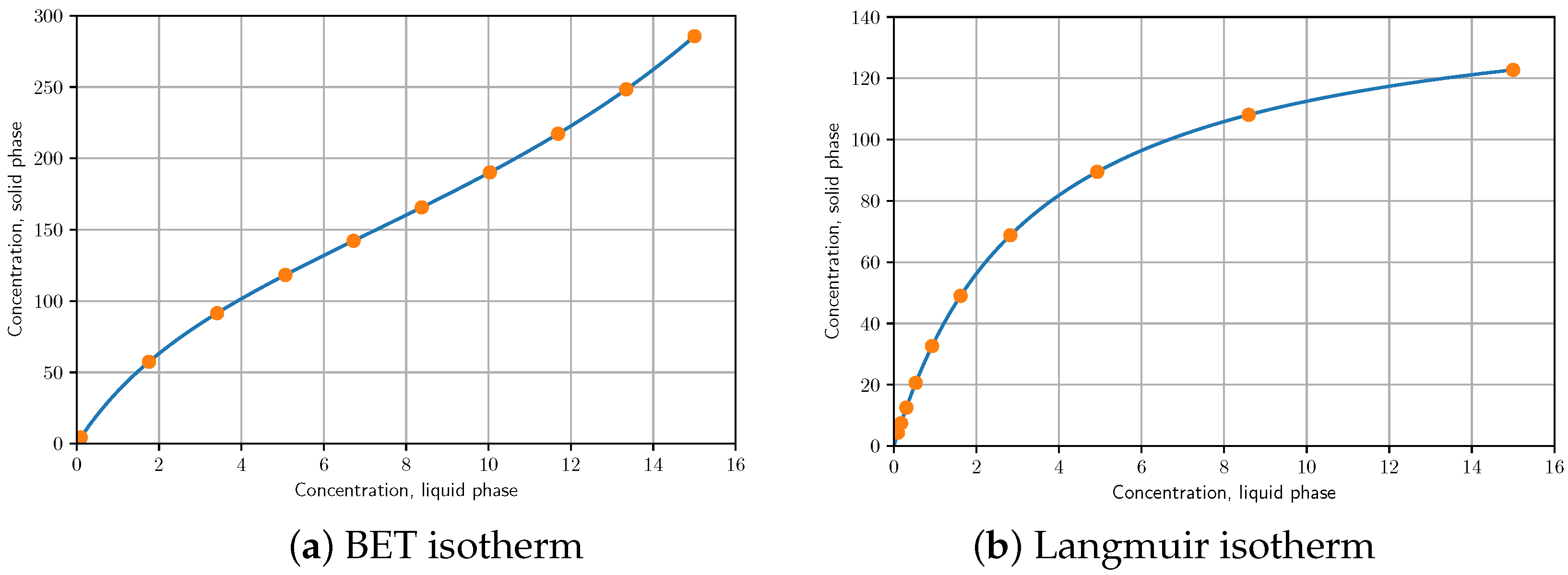
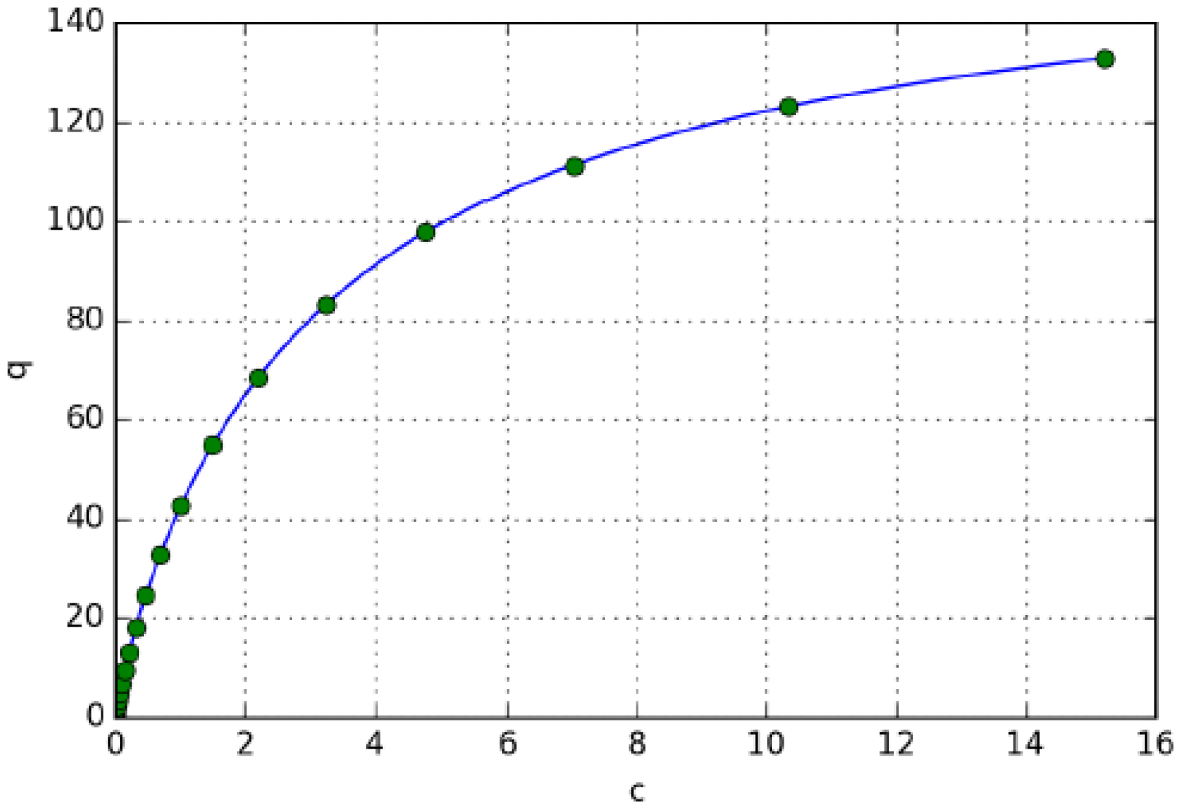
2.2. Models of Adsorption Isotherms
2.3. Determination of Isotherms by the Inverse Method
3. Results and Discussion
3.1. Distribution of Isotherm Points
- 1
- linear distribution in the abscissa,
- 2
- logarithmic distribution in the abscissa.
- 3
- linear distribution in the abscissa,
- 4
- logarithmic distribution in the abscissa,
- 5
- logarithmic distribution in the ordinate.
3.2. Method Verification by Benchmark Isotherm
- saturation capacity of the first and second type of adsorption centres,
- adsorption equilibrium constants of the two different adsorption centers,
- injection time, min
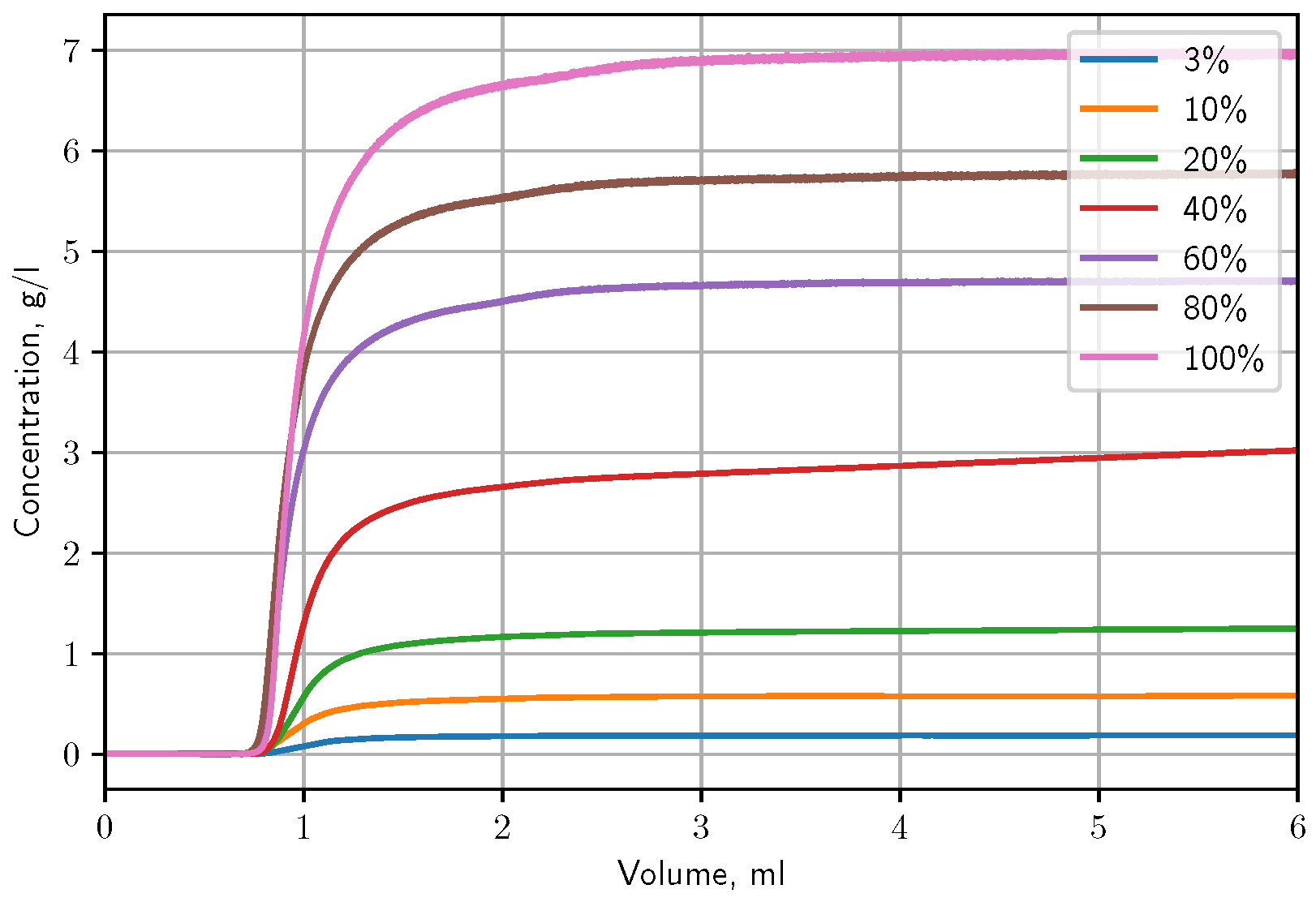
- injected concentration,
- columns length, cm
- linear velocity, cm/min
- phase ratio,
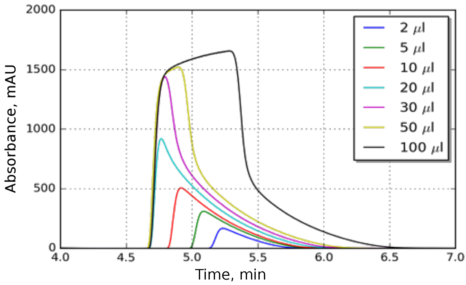
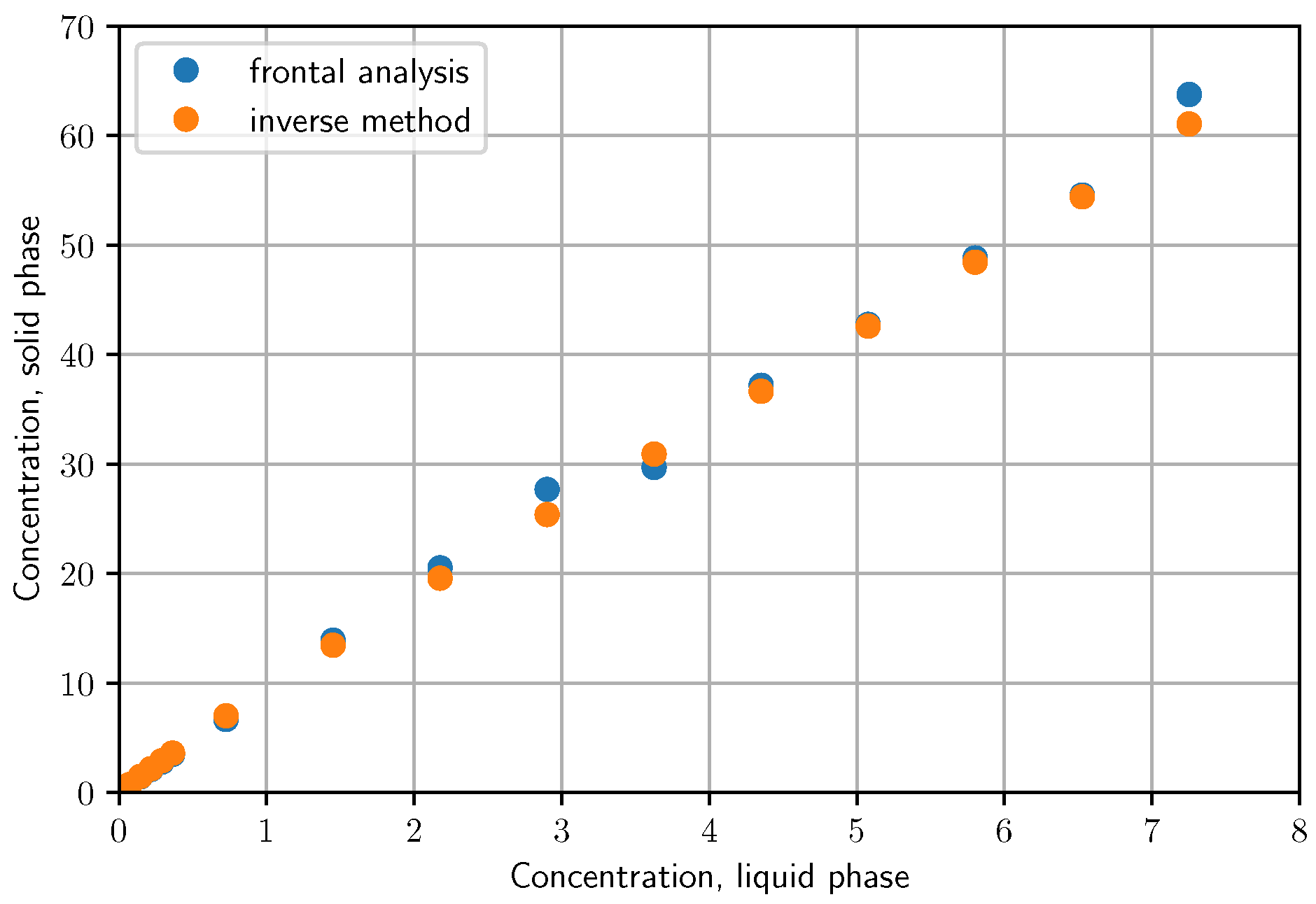
3.3. Determination of Butyl-Benzoate Isotherm
3.3.1. Isotherm Determination by Frontal Analysis
3.3.2. Determination of Butyl-Benzoate Isotherm by Unbiased Inverse Method
4. Materials and Methods
4.1. Instrumentation and Materials
4.2. Computation
5. Conclusions
Author Contributions
Funding
Institutional Review Board Statement
Informed Consent Statement
Data Availability Statement
Conflicts of Interest
Sample Availability
Abbreviations
| MDPI | Multidisciplinary Digital Publishing Institute |
| DOAJ | Directory of Open Access Journals |
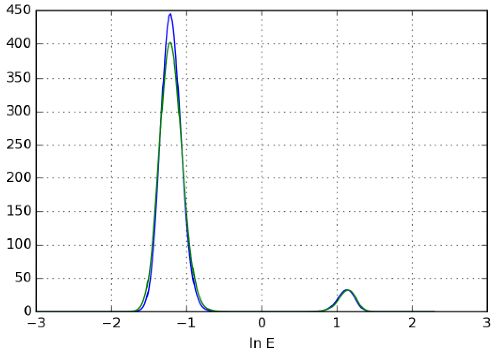
| AED | adsorption energy distributions |
| ECP | Elution by Characteristic Point |
| FA | Frontal Analysis |
| FACP | Frontal Analysis by Characteristic Point |
| HPLC | High Pressure Liquid Chromatography |
| IM | Inverse Method |
| RTM | Retention Time Method |
| SSR | Sum os Square Residuals |
References
- Guiochon, G.; Felinger, A.; Shirazi, D.G.; Katti, A.M. Fundamentals of Preparative and Nonlinear Chromatography; Academic Press: Amsterdam, The Netherlands, 2006. [Google Scholar]
- Carta, G. Scale-Up and Optimization in Preparative Chromatography: Principles and Biopharmaceutical Applications. J. Am. Chem. Soc. 2003, 11, 3398–3399. [Google Scholar] [CrossRef]
- Samuelsson, J.; Undin, T.; Fornstedt, T. Expanding the elution by characteristic point method for determination of various types of adsorption isotherms. J. Chromatogr. A 2011, 1218, 3737–3742. [Google Scholar] [CrossRef] [PubMed]
- Fornstedt, T. Characterization of adsorption processes in analytical liquid–solid chromatography. J. Chromatogr. A 2010, 1217, 792–812. [Google Scholar] [CrossRef] [PubMed]
- Sing, K.; Everett, D.; Haul, R.; Moscou, L.; Pierotti, R.; Rouquerol, J. Reporting physisorption data for gas/solid systems with special reference to the determination of surface area and porosity. Pure Appl. Chem. 1985, 57, 603–619. [Google Scholar] [CrossRef]
- Blahovec, J.; Yanniotis, S. Modified classification of sorption isotherms. J. Food Eng. 2009, 91, 72–77. [Google Scholar] [CrossRef]
- Samuelsson, J.; Arnell, R.; Fornstedt, T. Potential of adsorption isotherm measurements for closer elucidating of binding in chiral liquid chromatographic phase systems. J. Sep. Sci. 2009, 32, 1491–1506. [Google Scholar] [CrossRef]
- James, D.H.; Phillips, C.S.G. The chromatography of gases and vapours. Part III. The determination of adsorption isotherms. J. Chem. Soc. 1954, 1066–1070. [Google Scholar] [CrossRef]
- Glueckauf, E. Theory of chromatography. Part 10.—Formulæ for diffusion into spheres and their application to chromatography. J. Chem. Soc. Faraday Trans. 1951, 51, 1540–1551. [Google Scholar] [CrossRef]
- Cremer, E.; Huber, H. Messung von Adsorptionsisothermen an Katalysatoren bei hohen Temperaturen mit Hilfe der Gas-Festkörper-Eluierungschromatographie. Angew. Chem. 1961, 73, 461–465. [Google Scholar] [CrossRef]
- Helfferich, F. Travel of molecules and disturbances in chromatographic columns: A paradox and its resolution. J. Chem. Educ. 1964, 41, 410. [Google Scholar] [CrossRef]
- Golshan-Shirazi, S.; Guiochon, G. Experimental characterization of the elution profiles of high concentration chromatographic bands using the analytical solution of the ideal model. Anal. Chem. 1989, 61, 462–467. [Google Scholar] [CrossRef]
- Seidel-Morgenstern, A. Experimental determination of single solute and competitive adsorption isotherms. J. Chromatogr. A 2004, 1037, 255–272. [Google Scholar] [CrossRef]
- Dose, E.V.; Guiochon, G. Calibrating detector responses using chromatographic peak shapes. Anal. Chem. 1990, 62, 816–820. [Google Scholar] [CrossRef]
- Felinger, A.; Cavazzini, A.; Guiochon, G. Numerical determination of the competitive isotherm of enantiomers. J. Chromatogr. A 2003, 986, 207–225. [Google Scholar] [CrossRef] [PubMed]
- Felinger, A.; Zhou, D.; Guiochon, G. Determination of the single component and competitive adsorption isotherms of the 1-indanol enantiomers by the inverse method. J. Chromatogr. A 2003, 1005, 35–49. [Google Scholar] [CrossRef] [PubMed]
- Forssén, P.; Arnell, R.; Fornstedt, T. An improved algorithm for solving inverse problems in liquid chromatography. Comput. Chem. Eng. 2006, 30, 1381–1391. [Google Scholar] [CrossRef]
- Haghpanah, R.; Rajendran, A.; Farooq, S.; Karimi, I.; Amanullah, M. Discrete equilibrium data from dynamic column breakthrough experiments. Ind. Eng. Chem. Res. 2012, 51, 14834–14844. [Google Scholar] [CrossRef]
- Stineman, R. A consistently well-behaved method of interpolation. Int. J. Creat. Comput. 1980, 6, 54–57. [Google Scholar]
- Forssén, P.; Fornstedt, T. A model free method for estimation of complicated adsorption isotherms in liquid chromatography. J. Chromatogr. A 2015, 1409, 108–115. [Google Scholar] [CrossRef]
- Gao, W.; Engell, S. Estimation of general nonlinear adsorption isotherms from chromatograms. Comput. Chem. Eng. 2005, 29, 2242–2255. [Google Scholar] [CrossRef]
- Horváth, K.; Fairchild, J.N.; Kaczmarski, K.; Guiochon, G. Martin-Synge algorithm for the solution of equilibrium-dispersive model of liquid chromatography. J. Chromatogr. A 2010, 1217, 8127–8135. [Google Scholar] [CrossRef] [PubMed]
- van Deemter, J.; Zuiderweg, F.; Klinkenberg, A. Longitudinal diffusion and resistance to mass transfer as causes of nonideality in chromatography. Chem. Eng. Sci. 1956, 5, 271–289. [Google Scholar] [CrossRef]
- Giddings, J. Dynamics of Chromatography; CRC Press: Boca Raton, FL, USA, 1965. [Google Scholar]
- Haarhoff, P.C.; Van der Linde, H.J. Concentration Dependence of Elution Curves in Non-Ideal Gas Chromatography. Anal. Chem. 1966, 38, 573–582. [Google Scholar] [CrossRef]
- Horváth, K.; Vajda, P.; Felinger, A. Multilayer adsorption in liquid chromatography—The surface heterogeneity below an adsorbed multilayer. J. Chromatogr. A 2017, 1505, 50–55. [Google Scholar] [CrossRef] [PubMed]
- Nelder, J.A.; Mead, R. A Simplex Method for Function Minimization. Comput. J. 1965, 7, 308–313. [Google Scholar] [CrossRef]


| Number of Isotherm Points | |||||
|---|---|---|---|---|---|
| Scenario | 10 | 20 | 40 | 100 | 500 |
| 1 | 1.69 | 2.28 · 10−2 | |||
| 2 | 1.41 | ||||
| 3 | 0.46 | ||||
| 4 | 4270 | 156.6 | 31.05 | ||
| 5 | - | 1.54 | |||
Disclaimer/Publisher’s Note: The statements, opinions and data contained in all publications are solely those of the individual author(s) and contributor(s) and not of MDPI and/or the editor(s). MDPI and/or the editor(s) disclaim responsibility for any injury to people or property resulting from any ideas, methods, instructions or products referred to in the content. |
© 2023 by the authors. Licensee MDPI, Basel, Switzerland. This article is an open access article distributed under the terms and conditions of the Creative Commons Attribution (CC BY) license (https://creativecommons.org/licenses/by/4.0/).
Share and Cite
Horváth, S.; Lukács, D.; Farsang, E.; Horváth, K. Unbiased Determination of Adsorption Isotherms by Inverse Method in Liquid Chromatography. Molecules 2023, 28, 1031. https://doi.org/10.3390/molecules28031031
Horváth S, Lukács D, Farsang E, Horváth K. Unbiased Determination of Adsorption Isotherms by Inverse Method in Liquid Chromatography. Molecules. 2023; 28(3):1031. https://doi.org/10.3390/molecules28031031
Chicago/Turabian StyleHorváth, Szabolcs, Diána Lukács, Evelin Farsang, and Krisztián Horváth. 2023. "Unbiased Determination of Adsorption Isotherms by Inverse Method in Liquid Chromatography" Molecules 28, no. 3: 1031. https://doi.org/10.3390/molecules28031031