
Computation of Entropy Measures for Metal-Organic Frameworks
 ,
,  , , , and
Abstract
:1. Introduction
2. Entropy Measures
- The first -Banhatti entropy
- The second -Banhatti entropy
- The first K-hyper Banhatti entropy
- The second -hyper Banhatti entropy
- The first redefined Zagreb entropyLet . The first redefined Zagreb index (5) isThe first redefined Zagreb entropy is obtained using Equation (9)
- The second redefined Zagreb entropyLet . The second redefined Zagreb index (6) isThe second redefined Zagreb entropy is obtained using Equation (9)
- The third redefined Zagreb entropyLet . The third redefined Zagreb index (7) isThe third redefined Zagreb entropy is obtained by using Equation (9)
- Atom-bond sum connectivity EntropyLet . The atom-bond connectivity index (8) isThe atom-bond sum connectivity entropy is obtained using Equation (9)
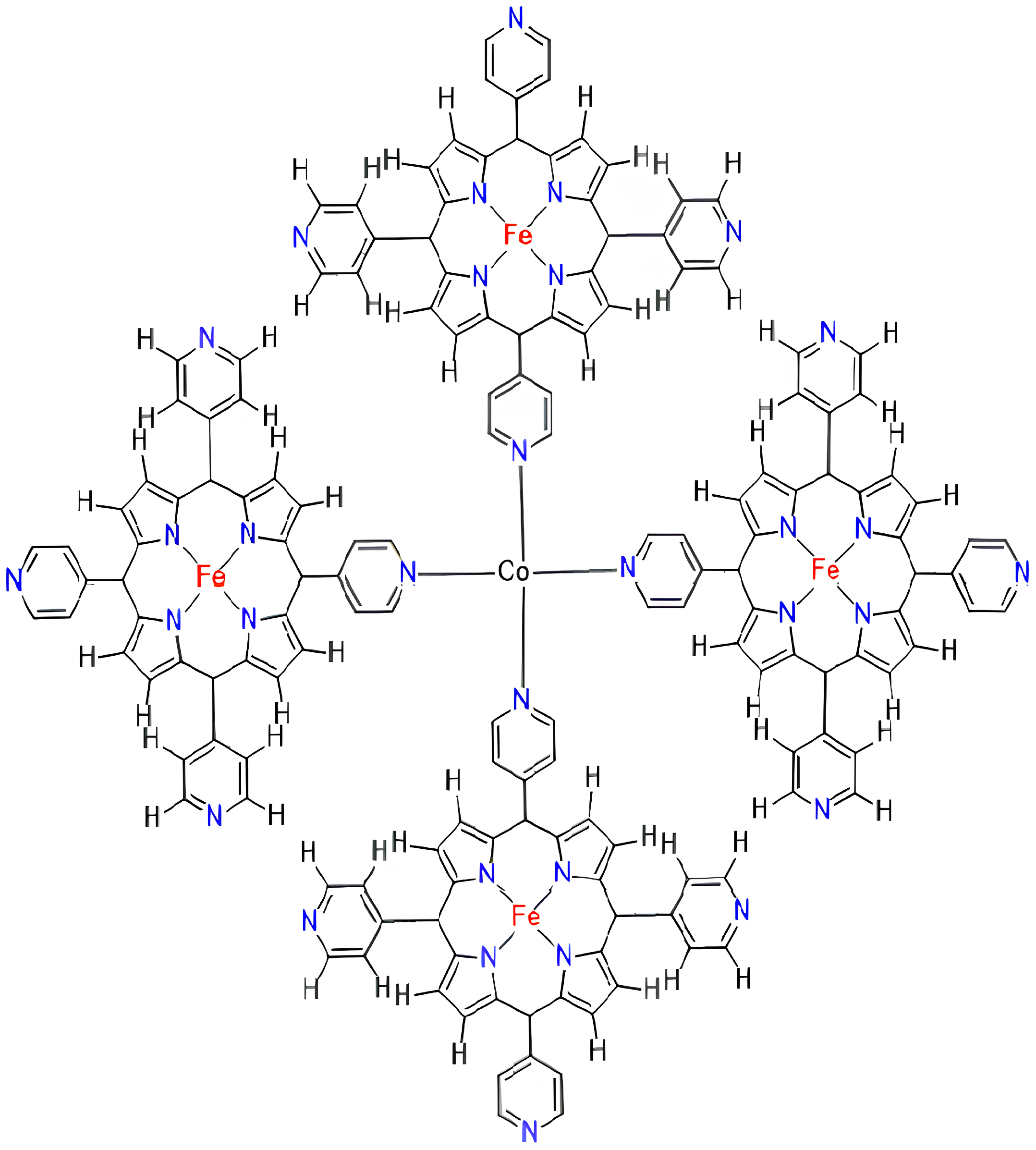
3. Entropy Measure of FeTPyP-Co
- The first -Banhatti entropy measure of
- The second K-Banhatti entropy measure of
- The first K-hyper Banhatti entropy measure of
- The second -hyper Banhatti entropy measure of
- The first redefined Zagreb entropy measure ofAfter differentiating Equation (26) at , we obtain
- The second redefined Zagreb entropy measure ofAfter differentiating Equation (28) at , we obtain
- The third redefined Zagreb entropy measure ofAfter differentiating Equation (30) at , we get
- Atom-bond sum connectivity entropy measure ofAfter differentiating Equation (32) at , we have
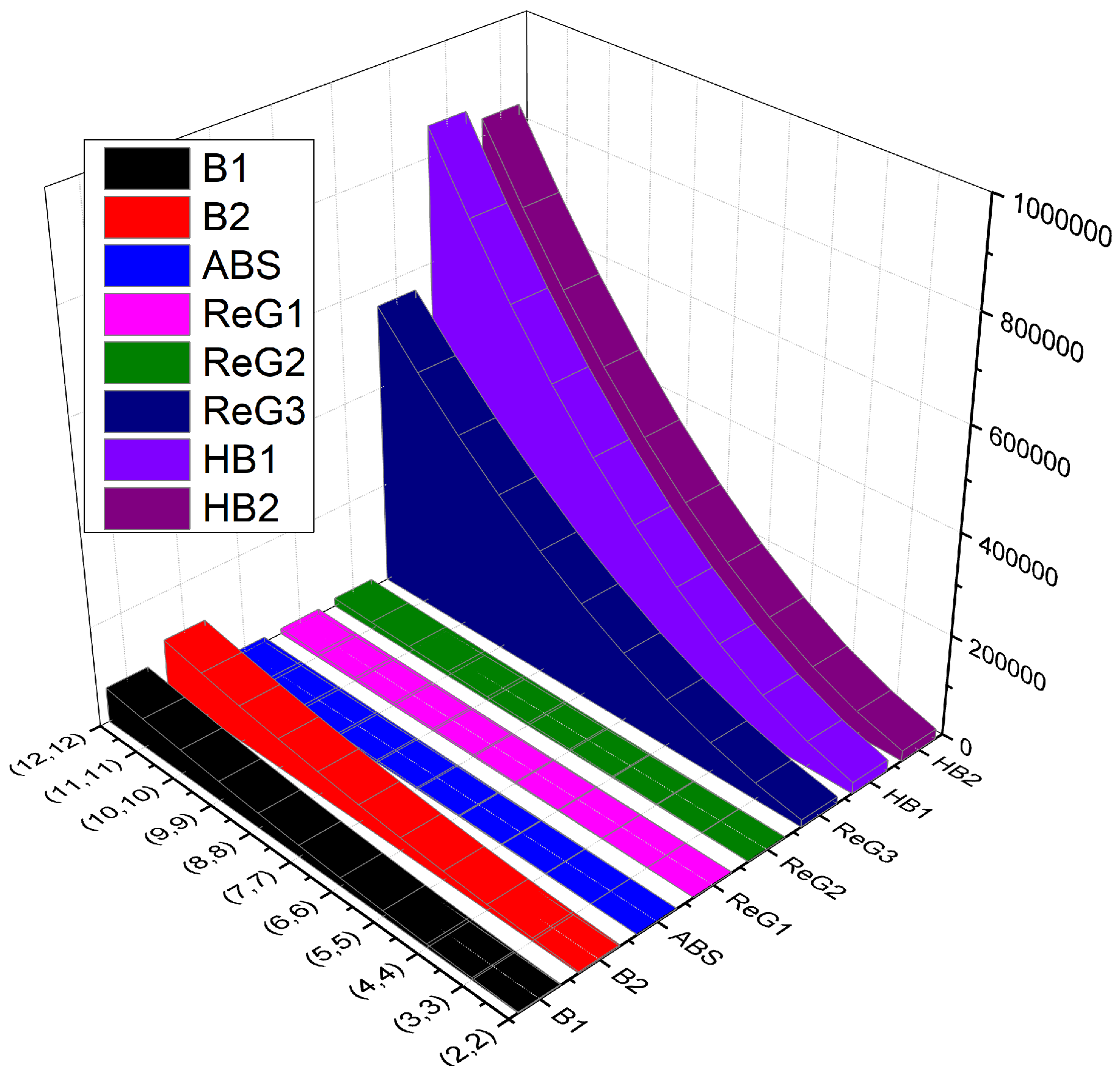
Comparison
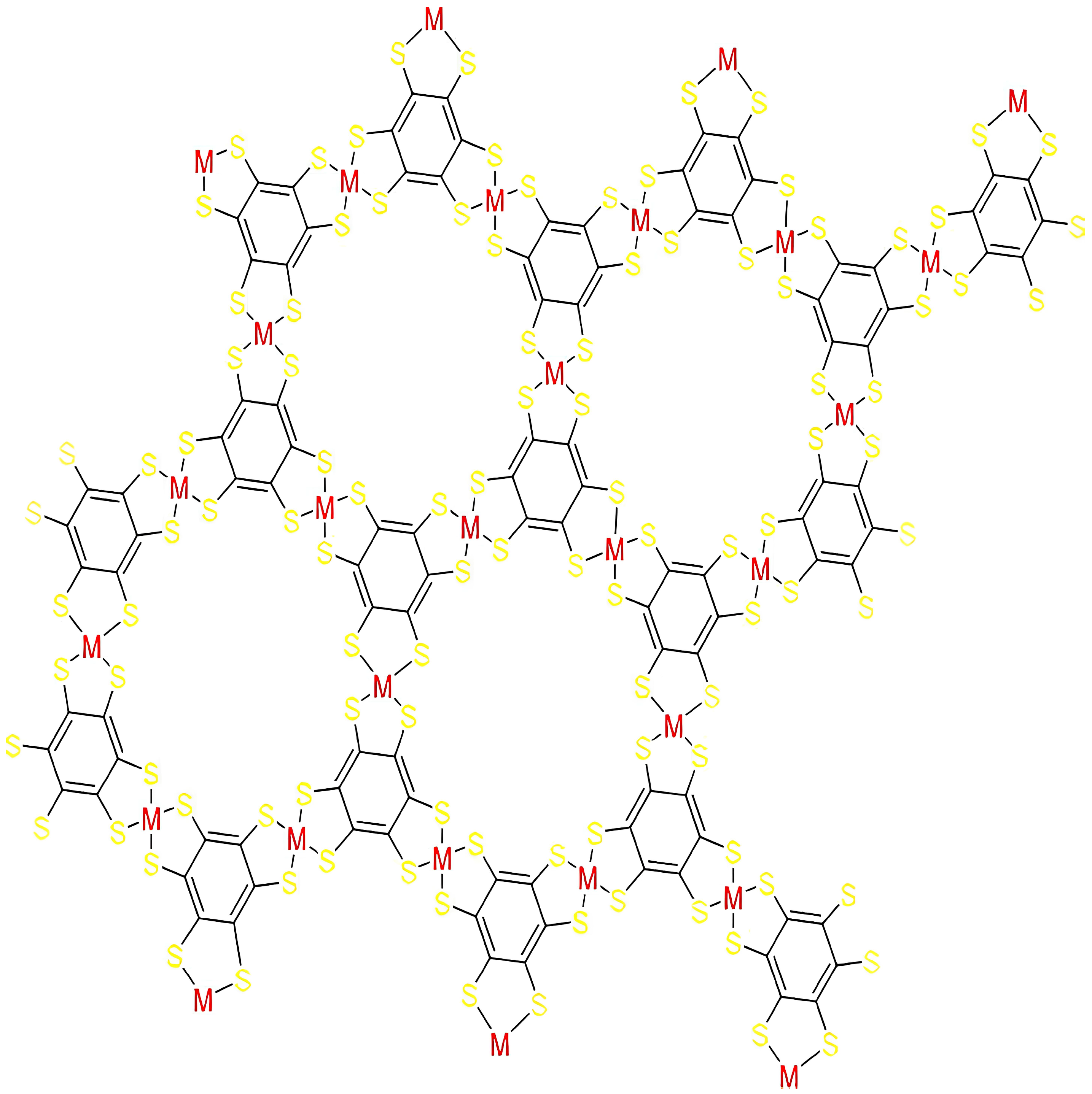
4. Entropy Measure of CoBHT (CO) Lattice
- The 1st -Banhatti entropy measure ofAfter differentiating Equation (34) at , we obtainTable 3. Atom-bonds partition of .
Types of Atom Bonds Cardinality of Atom bonds - The second -Banhatti entropy measure ofAfter differentiating Equation (36) at , we have
- The first -hyper Banhatti entropy measure ofAfter differentiating Equation (38) at , we get
- The second -hyper Banhatti entropy measure ofAfter differentiating Equation (40) at , we haveThe second K-hyper Banhatti entropy measure of is obtained in view of Equation (41) Table 3 and Equation (13):This gives
- The first redefined Zagreb entropy measure ofAfter differentiating Equation (43) at , we obtain the first redefined Zagreb index
- The second redefined Zagreb entropy measure ofAfter differentiating Equation (45) at , we obtain
- The third redefined Zagreb entropy measure ofAfter differentiating Equation (47) at , we obtain the third redefined Zagreb index
- Atom-bond sum connectivity entropy measure ofAfter differentiating Equation (49) at , we have

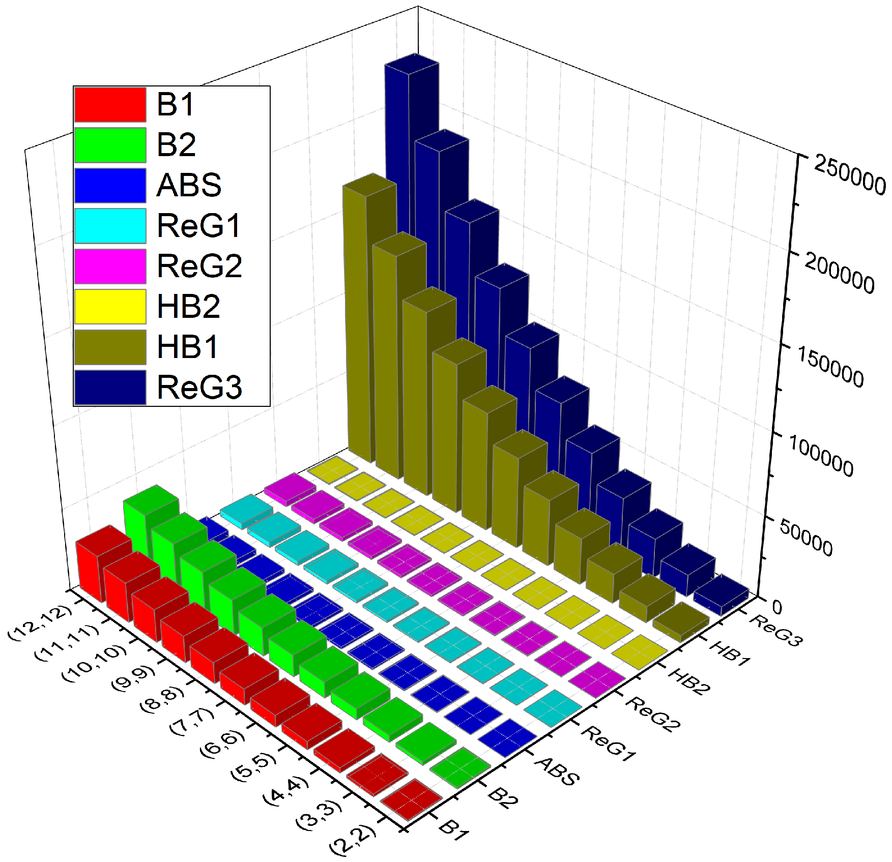
Comparison
5. Conclusions
Author Contributions
Funding
Institutional Review Board Statement
Informed Consent Statement
Data Availability Statement
Acknowledgments
Conflicts of Interest
Sample Availability
References
- Cook, T.R.; Zheng, Y.-R.; Stang, P.J. Metal–Organic Frameworks and Self-Assembled Supramolecular Coordination Complexes: Comparing and Contrasting the Design, Synthesis, and Functionality of Metal–Organic Materials. Chem. Rev. 2013, 113, 734–777. [Google Scholar] [CrossRef] [PubMed] [Green Version]
- Zhou, H.-C.; Long, J.R.; Yaghi, O.M. Introduction to Metal–Organic Frameworks; ACS Publications: Washington, DC, USA, 2012; Volume 112, pp. 673–674. [Google Scholar]
- Yasin, G.; Ibrahim, S.; Ajmal, S.; Ibraheem, S.; Ali, S.; Nadda, A.K.; Zhang, G.; Kaur, J.; Maiyalagan, T.; Gupta, R.K. Tailoring of electrocatalyst interactions at interfacial level to benchmark the oxygen reduction reaction. Coord. Chem. Rev. 2022, 469, 214669. [Google Scholar] [CrossRef]
- Yang, D.; Gates, B.C. Catalysis by Metal Organic Frameworks: Perspective and Suggestions for Future Research. ACS Catal. 2019, 9, 1779–1798. [Google Scholar] [CrossRef]
- Kumar, P.; Deep, A.; Kim, K.-H. Metal organic frameworks for sensing applications. Trac. Trends Anal. Chem. 2015, 73, 39–53. [Google Scholar] [CrossRef]
- Rani, P.; Husain, A.; Bhasin, K.K.; Kumar, G. Metal–Organic Framework-Based Selective Molecular Recognition of Organic Amines and Fixation of CO2 into Cyclic Carbonates. Inorg. Chem. 2022, 61, 6977–6994. [Google Scholar] [CrossRef] [PubMed]
- Mazaj, M.; Kaučič, V.; Zabukovec Logar, N. Chemistry of Metal-organic Frameworks Monitored by Advanced X-ray Diffraction and Scattering Techniques. Acta Chim. Slov. 2016, 63, 440–458. [Google Scholar] [CrossRef] [PubMed] [Green Version]
- Dolgopolova, E.A.; Brandt, A.J.; Ejegbavwo, O.A.; Duke, A.S.; Maddumapatabandi, T.D.; Galhenage, R.P.; Larson, B.W.; Reid, O.G.; Ammal, S.C.; Heyden, A.; et al. Electronic Properties of Bimetallic Metal–Organic Frameworks (MOFs): Tailoring the Density of Electronic States through MOF Modularity. J. Am. Chem. Soc. 2017, 139, 5201–5209. [Google Scholar] [CrossRef]
- Lee, K.; Park, J.; Song, I.; Yoon, S.M. The Magnetism of Metal–Organic Frameworks for Spintronics. Bull. Korean Chem. Soc. 2021, 42, 1170–1183. [Google Scholar] [CrossRef]
- Dhakshinamoorthy, A.; Navalon, S.; Asiri, A.M.; Garcia, H. Metal organic frameworks as solid catalysts for liquid-phase continuous flow reactions. Chem. Commun. 2020, 56, 26–45. [Google Scholar] [CrossRef]
- Sanford, M.S.; Love, J.A.; Grubbs, R.H. Mechanism and Activity of Ruthenium Olefin Metathesis Catalysts. J. Am. Chem. Soc. 2001, 123, 6543–6554. [Google Scholar] [CrossRef] [Green Version]
- Hu, M.-L.; Razavi, S.A.A.; Piroozzadeh, M.; Morsali, A. Sensing organic analytes by metal–organic frameworks: A new way of considering the topic. Inorg. Chem. Front. 2020, 7, 1598–1632. [Google Scholar] [CrossRef]
- Hosono, N.; Uemura, T. Metal-Organic Frameworks for Macromolecular Recognition and Separation. Matter 2020, 3, 652–663. [Google Scholar] [CrossRef]
- Zhang, Z.; Lou, Y.; Guo, C.; Jia, Q.; Song, Y.; Tian, J.-Y.; Zhang, S.; Wang, M.; He, L.; Du, M. Metal–organic frameworks (MOFs) based chemosensors/biosensors for analysis of food contaminants. Trends Food Sci. Technol. 2021, 118, 569–588. [Google Scholar] [CrossRef]
- Lawson, H.D.; Walton, S.P.; Chan, C. Metal–Organic Frameworks for Drug Delivery: A Design Perspective. ACS Appl. Mater. Interfaces 2021, 13, 7004–7020. [Google Scholar] [CrossRef]
- Tsai, H.; Shrestha, S.; Vilá, R.A.; Huang, W.; Liu, C.; Hou, C.-H.; Huang, H.-H.; Wen, X.; Li, M.; Wiederrecht, G.; et al. Bright and stable light-emitting diodes made with perovskite nanocrystals stabilized in metal–organic frameworks. Nat. Photonics 2021, 15, 843–849. [Google Scholar] [CrossRef]
- Wu, S.; Li, Z.; Li, M.-Q.; Diao, Y.; Lin, F.; Liu, T.; Zhang, J.; Tieu, P.; Gao, W.; Qi, F.; et al. 2D metal–organic framework for stable perovskite solar cells with minimized lead leakage. Nat. Nanotechnol. 2020, 15, 934–940. [Google Scholar] [CrossRef]
- Sakamaki, Y.; Tsuji, M.; Heidrick, Z.; Watson, O.; Durchman, J.; Salmon, C.; Burgin, S.R.; Beyzavi, H. Preparation and Applications of Metal–Organic Frameworks (MOFs): A Laboratory Activity and Demonstration for High School and/or Undergraduate Students. J. Chem. Educ. 2020, 97, 1109–1116. [Google Scholar] [CrossRef] [PubMed]
- Ghani, M.U.; Sultan, F.; Tag El Din, E.S.M.; Khan, A.R.; Liu, J.B.; Cancan, M. A Paradigmatic Approach to Find the Valency-Based K-Banhatti and Redefined Zagreb Entropy for Niobium Oxide and a Metal–Organic Framework. Molecules 2022, 27, 6975. [Google Scholar] [CrossRef] [PubMed]
- MacGillivray, L.R. (Ed.) Metal-Organic Frameworks: Design and Application; John Wiley & Sons: Hoboken, NJ, USA, 2010. [Google Scholar]
- James, S.L. Metal-organic frameworks. Chem. Soc. Rev. 2003, 32, 276–288. [Google Scholar] [CrossRef] [PubMed]
- Furukawa, H.; Cordova, K.E.; O’Keeffe, M.; Yaghi, O.M. The chemistry and applications of metal-organic frameworks. Science 2013, 341, 1230444. [Google Scholar] [CrossRef] [Green Version]
- Kitagawa, S. Metal–organic frameworks (MOFs). Chem. Soc. Rev. 2014, 43, 5415–5418. [Google Scholar]
- Liu, J.B.; Zhang, T.; Wang, Y.; Lin, W. The Kirchhoff index and spanning trees of Möbius/cylinder octagonal chain. Discret. Appl. Math. 2022, 307, 22–31. [Google Scholar] [CrossRef]
- Liu, J.B.; Bao, Y.; Zheng, W.T.; Hayat, S. Network coherence analysis on a family of nested weighted n-polygon networks. Fractals 2021, 29, 2150260. [Google Scholar] [CrossRef]
- Liu, J.B.; Zhao, J.; He, H.; Shao, Z. Valency-based topological descriptors and structural property of the generalized sierpiński networks. J. Stat. Phys. 2019, 177, 1131–1147. [Google Scholar] [CrossRef]
- Liu, J.-B.; Wang, C.; Wang, S.; Wei, B. Zagreb indices and multiplicative zagreb indices of eulerian graphs. Bull. Malays. Math. Sci. Soc. 2019, 42, 67–78. [Google Scholar] [CrossRef]
- Liu, J.B.; Zhao, J.; Min, J.; Cao, J. The Hosoya index of graphs formed by a fractal graph. Fractals 2019, 27, 1950135. [Google Scholar] [CrossRef]
- Liu, J.B.; Pan, X.F. Minimizing Kirchhoff index among graphs with a given vertex bipartiteness. Appl. Math. Comput. 2016, 291, 84–88. [Google Scholar] [CrossRef]
- Liu, J.B.; Pan, X.F.; Yu, L.; Li, D. Complete characterization of bicyclic graphs with minimal Kirchhoff index. Discret. Appl. Math. 2016, 200, 95–107. [Google Scholar] [CrossRef]
- Khan, A.R.; Ghani, M.U.; Ghaffar, A.; Asif, H.M.; Inc, M. Characterization of temperature indices of silicates. Silicon 2023, 1–7. [Google Scholar] [CrossRef]
- Chu, Y.M.; Khan, A.R.; Ghani, M.U.; Ghaffar, A.; Inc, M. Computation of Zagreb Polynomials and Zagreb Indices for Benzenoid Triangular & Hourglass System. Polycycl. Aromat. Compd. 2022; in press. [Google Scholar] [CrossRef]
- Wiener, H. Structural determination of paraffin boiling points. J. Am. Chem. Soc. 1947, 69, 17–20. [Google Scholar] [CrossRef]
- Vukičević, D.; Gašperov, M. Bond additive modeling 1. Adriatic indices. Croat. Chem. Acta 2010, 83, 243–260. [Google Scholar]
- Kulli, V.R. On K Banhatti indices of graphs. J. Comput. Math. Sci. 2016, 7, 213–218. [Google Scholar]
- Kulli, V.R.; On, K. On K hyper-Banhatti indices and coindices of graphs. Int. Res. J. Pure Algebra 2016, 6, 300–304. [Google Scholar]
- Kulli, V.R. On multiplicative K Banhatti and multiplicative K hyper-Banhatti indices of V-Phenylenic nanotubes and nanotorus. Ann. Pure Appl. Math. 2016, 11, 145–150. [Google Scholar]
- Ranjini, P.S.; Lokesha, V.; Usha, A. Relation between phenylene and hexagonal squeeze using harmonic index. Int. J. Graph Theory 2013, 1, 116–121. [Google Scholar]
- Saeed, N.; Long, K.; Mufti, Z.S.; Sajid, H.; Rehman, A. Degree-based topological indices of boron b12. J. Chem. 2021, 2021, 5563218. [Google Scholar] [CrossRef]
- Ali, A.; Furtula, B.; Redžepović, I.; Gutman, I. Atom-bond sum-connectivity index. J. Math. Chem. 2022, 60, 2081–2093. [Google Scholar] [CrossRef]
- Shannon, C.E. A mathematical theory of communication. Bell Syst. Tech. J. 1948, 27, 379–423. [Google Scholar] [CrossRef] [Green Version]
- Alam, A.; Ghani, M.U.; Kamran, M.; Shazib Hameed, M.; Hussain Khan, R.; Baig, A.Q. Degree-Based Entropy for a Non-Kekulean Benzenoid Graph. J. Math. 2022, 2022, 2288207. [Google Scholar]
- Rashid, T.; Faizi, S.; Zafar, S. Distance based entropy measure of interval-valued intuitionistic fuzzy sets and its application in multicriteria decision making. Adv. Fuzzy Syst. 2018, 2018, 3637897. [Google Scholar] [CrossRef]
- Hayat, S. Computing distance-based topological descriptors of complex chemical networks: New theoretical techniques. Chem. Phys. Lett. 2017, 688, 51–58. [Google Scholar] [CrossRef]
- Hu, M.; Ali, H.; Binyamin, M.A.; Ali, B.; Liu, J.B.; Fan, C. On distance-based topological descriptors of chemical interconnection networks. J. Math. 2021, 2021, 5520619. [Google Scholar] [CrossRef]
- Anjum, M.S.; Safdar, M.U. K Banhatti and K hyper-Banhatti indices of nanotubes. Eng. Appl. Sci. Lett. 2019, 2, 19–37. [Google Scholar] [CrossRef]
- Asghar, A.; Rafaqat, M.; Nazeer, W.; Gao, W. K Banhatti and K hyper Banhatti indices of circulant graphs. Int. J. Adv. Appl. Sci. 2018, 5, 107–109. [Google Scholar] [CrossRef]
- Kulli, V.R.; Chaluvaraju, B.; Boregowda, H.S. Connectivity Banhatti indices for certain families of benzenoid systems. J. Ultra Chem. 2017, 13, 81–87. [Google Scholar] [CrossRef]
- Liu, R.; Yang, N.; Ding, X.; Ma, L. An unsupervised feature selection algorithm: Laplacian score combined with distance-based entropy measure. In Proceedings of the 2009 Third International Symposium on Intelligent Information Technology Application, Nanchang, China, 21–22 November 2009; IEEE: Picataway, NJ, USA, 2009; Volume 3. [Google Scholar]
- Wang, D.; Ray, K.; Collins, M.J.; Farquhar, E.R.; Frisch, J.R.; Gómez, L.; Jackson, T.A.; Kerscher, M.; Waleska, A.; Comba, P.; et al. Nonheme oxoiron (IV) complexes of pentadentate N5 ligands: Spectroscopy, electrochemistry, and oxidative reactivity. Chem. Sci. 2013, 4, 282–291. [Google Scholar] [CrossRef] [Green Version]


| Types of Atom Bonds | ||||
|---|---|---|---|---|
| Cardinality |
| ABS | ||||||||
|---|---|---|---|---|---|---|---|---|
| (2,2) | 1754 | 2790 | 22,074 | 20,259 | 294.67 | 436.88 | 14,070 | 270.90 |
| (3,3) | 4090 | 6414 | 510,66 | 48,411 | 664.67 | 1004.14 | 32,922 | 614.18 |
| (4,4) | 7402 | 11,526 | 92,202 | 88,371 | 1182.67 | 1802.83 | 59,742 | 1096.37 |
| (5,5) | 11,690 | 18,126 | 145,482 | 140,139 | 1848.67 | 2832.94 | 94,530 | 1717.47 |
| (6,6) | 16,954 | 26,214 | 210,906 | 203,715 | 2662.67 | 4094.48 | 137,286 | 2477.48 |
| (7,7) | 23,194 | 35,790 | 288,474 | 279,099 | 3624.67 | 5587.46 | 188,010 | 3376.41 |
| (8,8) | 30,410 | 46,854 | 378,186 | 366,291 | 4734.67 | 7311.86 | 246,702 | 4414.25 |
| (9,9) | 38,602 | 59,406 | 480,042 | 465,291 | 5992.67 | 9267.68 | 313,362 | 5590.99 |
| (10,10) | 47,770 | 73,446 | 594,042 | 576,099 | 7398.67 | 11,454.94 | 387,990 | 6906.65 |
| (11,11) | 57,914 | 88,974 | 720,186 | 698,715 | 8952.67 | 13,873.63 | 470,586 | 8361.22 |
| (12,12) | 69,034 | 105,990 | 858,474 | 833,139 | 10,654.67 | 16,523.74 | 561,150 | 9954.70 |
| (2,2) | 776 | 1048 | 4424 | 136.28 | 118.28 | 155.33 | 5936 | 117.74 |
| (3,3) | 1776 | 2400 | 10,128 | 190.28 | 262.28 | 300.2 | 13,656 | 265.82 |
| (4,4) | 3184 | 4304 | 18,160 | 244.28 | 462.86 | 489.86 | 24,544 | 473.38 |
| (5,5) | 5000 | 6760 | 28,520 | 298.28 | 720 | 724.33 | 38,600 | 740.42 |
| (6,6) | 7224 | 9768 | 41,208 | 352.28 | 1033.71 | 1003.6 | 55,824 | 1066.93 |
| (7,7) | 9856 | 13,328 | 56,224 | 406.28 | 1404 | 1327.66 | 76,216 | 1452.91 |
| (8,8) | 12,896 | 17,440 | 73,568 | 460.28 | 1830.86 | 1696.53 | 99,776 | 1898.37 |
| (9,9) | 16,344 | 22,104 | 93,240 | 514.28 | 2314.28 | 2110.2 | 126,504 | 2403.31 |
| (10,10) | 20,200 | 27,320 | 115,240 | 568.28 | 2854.28 | 2568.66 | 156,400 | 2967.72 |
| (11,11) | 24,464 | 33,088 | 139,568 | 622.28 | 3450.86 | 3071.93 | 189,464 | 3591.61 |
| (12,12) | 29,136 | 39,408 | 166,224 | 676.28 | 4104 | 3620 | 225,696 | 4274.97 |
Disclaimer/Publisher’s Note: The statements, opinions and data contained in all publications are solely those of the individual author(s) and contributor(s) and not of MDPI and/or the editor(s). MDPI and/or the editor(s) disclaim responsibility for any injury to people or property resulting from any ideas, methods, instructions or products referred to in the content. |
© 2023 by the authors. Licensee MDPI, Basel, Switzerland. This article is an open access article distributed under the terms and conditions of the Creative Commons Attribution (CC BY) license (https://creativecommons.org/licenses/by/4.0/).
Share and Cite
Imran, M.; Khan, A.R.; Husin, M.N.; Tchier, F.; Ghani, M.U.; Hussain, S. Computation of Entropy Measures for Metal-Organic Frameworks. Molecules 2023, 28, 4726. https://doi.org/10.3390/molecules28124726
Imran M, Khan AR, Husin MN, Tchier F, Ghani MU, Hussain S. Computation of Entropy Measures for Metal-Organic Frameworks. Molecules. 2023; 28(12):4726. https://doi.org/10.3390/molecules28124726
Chicago/Turabian StyleImran, Muhammad, Abdul Rauf Khan, Mohamad Nazri Husin, Fairouz Tchier, Muhammad Usman Ghani, and Shahid Hussain. 2023. "Computation of Entropy Measures for Metal-Organic Frameworks" Molecules 28, no. 12: 4726. https://doi.org/10.3390/molecules28124726