Methods to Calculate Entropy Generation

Abstract

Entropy generation, formulated by combining the first and second laws of thermodynamics with an appropriate thermodynamic potential, emerges as the difference between a phenomenological entropy function and a reversible entropy function. The phenomenological entropy function is evaluated over an irreversible path through thermodynamic state space via real-time measurements of thermodynamic states. The reversible entropy function is calculated along an ideal reversible path through the same state space. Entropy generation models for various classes of systems—thermal, externally loaded, internally reactive, open and closed—are developed via selection of suitable thermodynamic potentials. Here we simplify thermodynamic principles to specify convenient and consistently accurate system governing equations and characterization models. The formulations introduce a new and universal Phenomenological Entropy Generation (PEG) theorem. The systems and methods presented—and demonstrated on frictional wear, grease degradation, battery charging and discharging, metal fatigue and pump flow—can be used for design, analysis, and support of diagnostic monitoring and optimization.

1. Introduction

System analyses based on energy conservation alone have been shown inadequate for consistent characterization of real, often nonlinear, system transformation. The introduction of the second law via the works of Carnot, Clapeyron [1], Clausius, Massieu [2] and others established thermodynamics as a field for consistent description of changes in a system undergoing any form of energy conversion. For centuries, classical thermodynamics has been restricted to equilibrium and near-equilibrium transformations. Defining a minimum condition for a system to exist or process to occur in nature, Rayleigh’s dissipation function [3], Onsager’s least energy dissipation [4] (an application of his reciprocal relations of microscopic reversibility) and Prigogine’s minimum entropy generation [5,6]—similar statements expressed as $\delta S^{\prime }=YdX/T$—set the stage for thermodynamic characterization of real system transformation, a field commonly known as irreversible thermodynamics. Here, $\delta S^{\prime }$ is entropy generation, Y is generalized force, dX is generalized displacement and T is temperature. The correlation between energy dissipation (or entropy generation) and system degradation—advanced and permanent disorganization of material structure—has been theorized and experimentally verified. Recently, several multi-disciplinary system characterizations have emerged, presenting experimental results consistent with entropy-based formulations. These works show high accuracies in analyzing active system transformations, with inconsistencies attributable to the often-used “steady state” assumption. While some long-running systems operate predominantly in pseudo-steady state, e.g., very high-cycle fatigue of steels, most loaded systems often transform unsteadily, limiting the applicability of energy conservation and steady-state entropy characterizations. Recent works by Osara and Bryant [7,8,9,10] using the Degradation-Entropy Generation (DEG) methodology [11] to assess battery degradation, grease degradation and metal fatigue, showed a near 100% accurate and consistent characterization of these systems undergoing severely abusive loads. DEG methods relate increments of degradation to increments of entropy generation. Instead of a “steady state” assumption, Osara and Bryant [7,8,9,10] augmented laws of thermodynamics with the thermodynamic potentials to formulate entropy generation. Methods to calculate entropy generation under general conditions for all systems are needed to enable real-time assessment of system transformation.

This article will develop entropy generation $\delta S^{\prime }$ for open and closed systems as the difference

$$\delta S^{\prime }={\delta \mathbb{S}}_{phen}-{d\mathbb{S}}_{rev}\ge 0$$

(1a)

between a phenomenological entropy generation function ${\delta \mathbb{S}}_{phen}$, evaluated via suitable measurements of variables over an irreversible path in a thermodynamic state space between initial and final (or current) thermodynamic states; and a reversible entropy function ${d\mathbb{S}}_{rev}$, evaluated over a reversible path in the same state space between the same initial and final states. The thermodynamic state space consists of any independent variables that characterize the thermodynamic state and all active irreversible dissipative processes. The reversible path for ${d\mathbb{S}}_{rev}$, which is the projection of the irreversible phenomenological path of ${\delta \mathbb{S}}_{phen}$ onto the reversible subspace, consists of the thermodynamic state variables of the phenomenological path sans the irreversible dissipative process variables. This approach will eliminate many tenuous “steady state” assumptions and loopholes in existing approaches. To obtain entropy generation $S^{\prime }$, Equation (1a) must be integrated between the initial and final/current states, with entropy functions ${\delta \mathbb{S}}_{phen}$ and ${d\mathbb{S}}_{rev}$ integrated over their respective paths. True reversibility excludes process rates and time effects, hence, the reversible path defined herein marks the theoretical limit of a real-time-based process via a linear function joining the initial and final states.

1.1. Local Equilibrium

Prigogine posited: given that true equilibrium is asymptotic for all real systems, every continuous macroscopic system is made up of elements for which observable state properties (such as temperature and pressure) can be instantaneously determined or measured, thereby rendering equilibrium formulations describing these properties valid for each element in the macrosystem. Each element is, therefore, in local equilibrium [5,6,12,13]. This theorem allows the extension of reversibility-based formulations to real systems, with entropy generation representation. While the system variables are spatial and temporal functions, many real systems operate with near-uniform internal properties, primarily changing with time.

1.2. States, Paths and Path (Line) Integrals

The following principles will be judicious to Section 2:

• Thermodynamics often involves changes in variables between two states. Variables include a set of the independent thermodynamic state variables Z chosen and measured for a particular system, and state dependent system properties which are functions of the states of Z. The Z characterize a system’s thermodynamic state and can include temperature T, pressure P, and number of moles N, among others. Changes in system properties such as energy E, entropy S, temperature T and ${\mathbb{S}}_{rev}$ use the exact differential d; are path independent, wherein changes in properties over an irreversible path (irr) are identical to changes in properties over a reversible path (rev), e.g., dE = dE_irr = dE_rev; and the line integral ${\int }_o^{f}dE=∆E=E_f-E_o$ depends only on the property values at the beginning and end states (o and f). This is the thermodynamic state principle.
• Path-dependent variables such as work W, heat transfer $Q,$ entropy generation $S^{\prime }$ and ${\mathbb{S}}_{phen}$ depend on what occurs along the path between states o and f, and use the inexact differential $\delta$ such that ${\int }_o^f\delta W=W$ must be accumulated over all instants of time t along the (assumed known) transformation path between times $t_o$ and $t_f$. The path-dependent parameters will depend on a set of variables $\mathcal{Z}$= {Z$,{\zeta }_k$} assumed to be time dependent, observable, and measurable. The Z characterize the thermodynamic state, whereas the ${\zeta }_k$ characterize any active irreversible dissipative processes. Via a suitable numerical integration such as the trapezoid rule, with the $\mathcal{Z}\left(t\right)$ = {Z(t), ${\zeta }_k\left(t\right)$} measured as points $\mathcal{Z}\left(t_j\right)$= {Z$(t_j)$, ${\zeta }_k(t_j)\}$ suitably spaced at time instants $t_o<$ $t_j$ < $t_f$ in accord with the sampling theorem [14], the increments $\delta W$ can be accumulated into the line integral ${\int }_o^f\delta W=W$.
• Exact differentials $dE$, state functions of the independent state variables Z(t), if intractable, can be numerically integrated over the (ideal) reversible path per methods of the prior paragraph. The reversible path must transit states o to f in quasi-equilibrium and be continuous and maximally smooth over time, which can be approximated by linear functions with slope determined by the end states, for example, if $dE\left(t\right)=dE(\mathit{Z}(t))$, components of Z(t) with slope $\frac{{Z(t}_f)-{Z(t}_o)}{t_f-t_o}$ where ${Z(t}_f)$ and ${Z(t}_o)$ must be measured or known at the beginning and final times $t_o$ and $t_f$. With this, the line integral ${\int }_o^{f}dE={\int }_{t_o}^{t_f}\frac{dE}{dt}dt={\int }_{t_o}^{t_f}\sum _Z\frac{dE}{dZ}\frac{dZ}{dt}dt=\sum _Z\frac{{Z(t}_f)-{Z(t}_o)}{t_f-t_o}{\int }_{t_o}^{t_f}\frac{dE}{dZ}dt$, where sum index Z denotes a sum over all the components of Z, and dE/dZ must be evaluated at each time instant $t_o<$ $t_j$ < $t_f$ along the reversible path.
• For reversible processes ${d\mathbb{S}}_{rev}$ with initial and final states ${{d\mathbb{S}}_{rev}}_o$ and ${{d\mathbb{S}}_{rev}}_f$, ${d\mathbb{S}}_{rev}(t)=\frac{{{d\mathbb{S}}_{rev}}_f-{{d\mathbb{S}}_{rev}}_o}{t_f-t_o}(t-t_o)+{{d\mathbb{S}}_{rev}}_o$ satisfies the reversible path approximations of item 3.
• A phenomenological path (phen) through the thermodynamic state space enclosing $\mathcal{Z}$= {Z$,{\zeta }_k$} defined in item 2 includes nonzero ${\zeta }_k\left(t\right)$. A reversible path (rev) in the reversible subspace {Z} of $\mathcal{Z}$ [15] involves only the thermodynamic states Z_rev, not the ${\zeta }_k$. The projection of the set of points $\mathcal{Z}\left(t_j\right)$= {Z$\left(t_j\right)$, ${\zeta }_k(t_j)\}$ that comprise an irreversible phenomenological path onto the reversible subspace is the set of points {${\mathit{Z}}_{\mathit{r}\mathit{e}\mathit{v}}\left(t_j\right)\}$ [15]. The system inputs, active mechanisms and dynamics are determined by the phenomenological path.

These principles are based on classical approaches [2,16,17]. While classical theories are limited to equilibrium and near-equilibrium states, we here introduce concurrent physically observable states to characterize real, often highly dissipative, far-from-equilibrium systems.

2. Irreversible Thermodynamics and Entropy Generation

2.1. Combining Internal Energy and Entropy Balances

For a stationary thermodynamic system (open and closed), excluding gravitational effects, the first law of thermodynamics

$$dU=\sum \delta Q-\sum \delta W+\sum {\left(u+Pv\right)dN}_e+\sum {\mu }_{k}d{N}_k,$$

(2)

balances $dU$, the change in overall system “internal” energy. Here $\sum \delta Q$ is the sum of all heat exchanges across the system boundary, $\sum \delta W$ is the sum of all work transfers across the system boundary, $\sum {\left(u+Pv\right)dN}_e$ is the sum of energy transfers by matter flows ${dN}_e$ across the system boundary (for open systems only), and $\sum {\mu }_{k}d{N}_k$ is the sum of all compositional energy changes within the system boundary. Embedded in the compositional change term $\sum {\mu }_{k}d{N}_k$ are, in terms of mole number $N_k$ of species k, changes in the quantity of matter due to chemical reactions ${{dN}^r}_k$ and ionic mass diffusions within the system boundary ${{dN}^d}_k$, i.e., $d{N}_k={{dN}^r}_k+{{dN}^d}_k$, where ${N^r}_k$ and ${N^d}_k$ are reactive and internally diffusive species, respectively. Also, u is molar internal energy, P is pressure, v is molar volume and $\mu$ is chemical potential. The product Pv is termed the flow work in open systems. Via the molar mass, Equation (2) can be re-written in terms of mass m. Inexact differential $\delta$ indicates path-dependent variables.

A statement of the second law—the Clausius inequality—gives the change in entropy of a closed system as $dS\ge \frac{\delta Q}{T}$ where δQ/T is entropy flow by heat transfer, which can be positive or negative depending on the transfer direction, and T is the temperature of the boundary where the energy/entropy transfer takes place. Via the thermodynamic state principle—item 1 of Section 1.2—and the entropy balance [5,6,12], entropy change accompanying an open system process can be evaluated along a real and often nonlinear irreversible path (irr) as

$$dS=d{S}_{irr}=\frac{\delta Q}{T}+\frac{\left(u+Pv\right){dN}_e}{T}+\delta S^{\prime }={\delta S}_Q+{dS}_{N_e}+\delta S^{\prime },$$

(3)

where ${\delta S}_Q=\frac{\delta Q}{T}$ is entropy transfer via heat, ${dS}_{N_e}=\frac{\left(u+Pv\right){dN}_e}{T}$ is entropy transfer via mass, and $\delta S^{\prime }$ is internal entropy generation which always accompanies permanent change and structural disorganization of the evolving system. While dS, ${\delta S}_Q$ and ${dS}_{N_e}$ can be positive or negative, the second law asserts $\delta S^{\prime }\ge 0$. Without a priori knowledge of the entropy generation, change along the irreversible path, Equation (3), cannot be determined. Along a reversible rev (ideal and linear) path with $\delta S^{\prime }=0$,

$$dS=d{S}_{rev}=\frac{\delta Q_{rev}}{T}+\frac{{\left(u+Pv\right)}_{rev}{dN}_e}{T}={\delta S}_{Q,rev}+{dS}_{N_e,rev}.$$

(4)

Substituting $\delta W=\sum Y_{l}d{X}_l$ [18] for external/boundary works including compression $PdV$, strain work $V\sigma d\epsilon$, electrical work $\nu dq$ and others into Equation (2) and combining with entropy Equation (3) gives the combined first and second laws as

$$T\delta S^{\prime }+dU=TdS-\sum Y_{l}d{X}_l +\sum {\mu }_{k}d{N}_k=T{\delta \mathbb{S}}_{U,phen}(S,X_l,N_k),$$

(5)

where Y_l are intensive variables such as pressure P, strength/stress $\sigma$, voltage $\nu$, etc.; $X_l$ are the system’s extensive variables such as volume V, strain $\epsilon$, charge $q$; and $T{\delta \mathbb{S}}_U\left(S,X_l,N_k\right)$, a path-dependent inexact differential, is defined by and equal to the middle expression of Equation (5). The script notation distinguishes ${\mathbb{S}}_{\mathit{U}}$ as an entropy related function of the independent variables in parenthesis. Subscript $phen$ indicates evaluation along the phenomenological path, the observable path where the independent states and dissipative process variables are available and measured at each instant. Since the product of temperature and entropy change ($TdS$) in Equation (5) subsumes the heat and flow transfer terms in Equations (2) and (3), Equation (5) is valid for all systems, open and closed [7,8,9,10,12]. Equation (5), which governs the system along an irreversible path, has a pair of unknowns $\delta S^{\prime }>0$ and $dU$; all other terms are observable and can be measured, as shown later.

To solve, a second independent equation will arise via $\delta S^{\prime }=0$ [7,8,9,10] applied to Equation (5). Recalling the thermodynamic state principle, all process paths between the same initial and end states must have the same difference between states: $dU={dU}_{irr}$=${ dU}_{rev}$, $dS={dS}_{irr}={dS}_{rev}$, etc., whether the path be reversible or irreversible. Substituting difference values into Equation (5) with $\delta S^{\prime }=0$, and solving yields

$$dU={dU}_{rev}=Td{S}_{rev}-\sum Y_{l,rev}d{X}_l +\sum {\mu }_{k,rev}d{N}_k=T{d\mathbb{S}}_{U,rev}(S,X_l,N_k),$$

(6)

where subscript rev indicates a quantity evaluated under reversible conditions. (Classical thermodynamics calculates entropy change along a reversible path, Equations (4) and (6), with reversible energy changes conveniently calculated via ideal response to loads, e.g., elastic deformation or non-saturating magnetics). Substituting $dU$=${ dU}_{rev}$ from Equation (6) into Equation (5) and rearranging yields entropy generation

$$\delta S^{\prime }=dS-\frac{\sum Y_{l}d{X}_l }{T}+\frac{\sum {\mu }_{k}d{N}_k}{T}-\frac{d{U}_{rev}}{T}={\delta \mathbb{S}}_{U,phen}(S,X_l,N_k)-{d\mathbb{S}}_{U,rev}(S,X_l,N_k)$$

(7)

for all systems. The middle equalities of Equations (5) and (6) serve to evaluate the right-side terms of Equation (7).

In Equations (3) and (4) and forthcoming entropy formulations, summation signs ∑ indicating multiple heat and mass flow terms are omitted for convenience.

2.2. Entropy Generation of Various System Classes via Thermodynamic Potentials

To evaluate entropy generation, Equation (7) requires the system’s changes of entropy $dS$ and internal energy $d{U}_{rev}$. These are difficult to determine, especially for non-thermal and multi-component systems [16], necessitating the widely used “steady state” assumption ($dS=d{U}_{rev}=0$) that led to Prigogine’s stationary nonequilibrium transformation or minimum entropy generation $\delta {S^{\prime }}_{min}=\frac{PdV}{T}+\frac{\sum {\mu }_{k}d{N}_k}{T}$ for a reacting compressible system [5,6,12]. Via Legendre transforms, equivalent forms of Equations (5) and (7) are derived in terms of observable, measurable and more easily controllable system properties such as temperature and pressure [16] for all systems, open or closed, steady or unsteady. The thermodynamic potentials (with PV work replaced by generalized YX work)––enthalpy $H=U+YX$, Helmholtz free energy $A=U–TS$ and Gibbs free energy $G=U+YX–TS$––are differentiated and solved for $dU$, the result of which is then inserted into Equation (5) to get:

$$T\delta S^{\prime }+dH=TdS+\sum ^l{X}_{l}d{Y}_l+\sum ^k{\mu }_{k}d{N}_k=T{\delta \mathbb{S}}_{H,phen}\left(S,Y_l,N_k\right)$$

(8a)

$$T\delta S^{\prime }+dA=-S_{A}dT-\sum ^l{Y}_{l}d{X}_l+\sum ^k{\mu }_{k}d{N}_k=T{\delta \mathbb{S}}_{A,phen}(T,X_l,N_k)$$

(8b)

$$T\delta S^{\prime }+dG=-S_{G}dT+\sum ^l{X}_{l}d{Y}_l+\sum ^k{\mu }_{k}d{N}_k=T{\delta \mathbb{S}}_{G,phen}(T,Y_l,N_k)$$

(8c)

Analogous to the operations performed on Equation (5) that led to Equation (7), similar operations performed on Equations (8) and solved for $\delta S^{\prime }$ render

$$\delta S^{\prime }=dS+\frac{\sum X_{l}d{Y}_l }{T}+\frac{\sum {\mu }_{k}d{N}_k}{T}-\frac{d{H}_{rev}}{T}={\delta \mathbb{S}}_{H,phen}(S,Y_l,N_k)-{d\mathbb{S}}_{H,rev}(S,Y_l,N_k)$$

(9a)

$$\delta S^{\prime }=\frac{-S_{A}dT}{T}-\frac{\sum Y_{l}d{X}_l }{T}+\frac{\sum {\mu }_{k}d{N}_k}{T}-\frac{{dA}_{rev}}{T}={\delta \mathbb{S}}_{A,phen}(T,X_l,N_k)-{d\mathbb{S}}_{A,rev}(T,X_l,N_k)$$

(9b)

$$\delta S^{\prime }=\frac{-S_{G}dT}{T}+\frac{\sum X_{l}d{Y}_l }{T}+\frac{\sum {\mu }_{k}d{N}_k}{T}-\frac{d{G}_{rev}}{T}={\delta \mathbb{S}}_{G,phen}(T,Y_l,N_k)-{d\mathbb{S}}_{G,rev}(T,Y_l,N_k).$$

(9c)

Equations (7) and (9), of the form of Equation (1a), require:

• ${\delta \mathbb{S}}_{phen}$: evaluated via the expressions of the middle equalities of Equations (5) and (8) at points over the irreversible phenomenological path defined in items 2 and 5 of Section 1.2, where salient quantities can be measured.
• ${d\mathbb{S}}_{rev}$: evaluated as an exact differential over a reversible path between the beginning and final values of the irreversible path for ${\delta \mathbb{S}}_{phen}$, as discussed in list items 3, 4 and 5 of Section 1.2. Here, the independent states in the parentheses of Equations (5) and (8) are linear in time, as per items 3 and 4 of Section 1.2.

2.3. Phenomenological Entropy Generation Theorem

The results of Equations (7) and (9) can be summarized as the

Phenomenological Entropy Generation (PEG) Theorem: 

Spontaneous entropy (and energy) changes along the (observable) phenomenological path is the sum of the ideal (linear, reversible transformation) entropy and the internally generated entropy, respectively:

$${\delta \mathbb{S}}_{phen}={d\mathbb{S}}_{rev}+\delta S^{\prime },$$

(1b)

which can be solved for entropy generation, as in Equation (1a), repeated here as

$$\delta S^{\prime }={\delta \mathbb{S}}_{phen}-{d\mathbb{S}}_{rev}\ge 0,$$

where, for energy extraction/decomposition or system loading, $\left({d\mathbb{S}}_{rev}\le {\delta \mathbb{S}}_{phen}\right)<0$, and for energy addition/formation, $0<\left({d\mathbb{S}}_{rev}\le {\delta \mathbb{S}}_{phen}\right)$. Only end state measurements of system variables (before and after process interaction) are required for evaluation of ${d\mathbb{S}}_{rev}$ (see items 3 and 4 of Section 1.2), unlike ${\delta \mathbb{S}}_{phen}$ which requires an instantaneous account of all active processes. Note that a system’s energy change and entropy change during a process can be negative or positive, depending on the direction of energy or entropy flow across system boundaries.

2.4. Phenomenological Entropy Generation Functions for Various System Classes

2.4.1. Thermal Systems: Internal Energy and Enthalpy

Thermal systems include heat engines (thermal energy to mechanical work), heat pumps (mechanical work to thermal energy) and hydrocarbon fuels (chemical energy to thermal energy). Convenient for fuels and open systems is enthalpy H [16], which replaces volume with pressure as independent variable and measures the amount of thermal energy in a system. In a chemical reaction, change in enthalpy sums the heat absorbed or released by the reaction, by non-boundary deforming interactions, and by change in internal compositional energies. A fuel source’s heating value is its enthalpy of combustion. For heat energy, the external work terms $\frac{\sum Y_{l}d{X}_l }{T}$ in Equations (8a) and (7) are neglected and ${dH}_{rev}$ and ${dU}_{rev}$, the maximum/minimum theoretical thermal energies available are often specified in tables, e.g., standard enthalpy of formation of pure substances [19], standard enthalpy of reaction, or standard enthalpy of combustion or heating value of fuels [20]. The heat entropy change $dS$ in Equations (7) and (9a) is evaluated via Equation (4) using the thermal energy balance $\delta Q=CdT$—for heat flow to or from a thermal system at uniform temperature with no heat generation—rendering ${dS}_{rev}=\frac{C_{rev}dT}{T}+\frac{{\left(u+Pv\right)}_{rev}{dN}_e}{T}$. For a given transformation and flow, ${dH}_{rev}$ and ${dU}_{rev}$ are constants, hence the middle set of terms of Equations (7) and (9a) are extracted to obtain the phenomenological entropy generation functions:

$${\delta \mathbb{S}}_{U,phen}=\frac{C_{rev}dT}{T}+\frac{{\left(u+Pv\right)}_{rev}{dN}_e}{T}-\frac{\sum Y_{l}d{X}_l }{T}+\frac{\sum {\mu }_{k}d{N}_k}{T}$$

(10a)

and

$${\delta \mathbb{S}}_{H,phen}=\frac{C_{rev}dT}{T}+\frac{{\left(u+Pv\right)}_{rev}{dN}_e}{T}+\frac{\sum X_{l}d{Y}_l }{T}+\frac{\sum {\mu }_{k}d{N}_k}{T}.$$

(10b)

$C_{rev}$ is the heat capacity (which can be obtained at standard room temperature and pressure) and ${\left(u+Pv\right)}_{rev}$ is the open-system flow enthalpy which, in the case of evaporation, is the latent heat of vaporization. Equation (10a) applies to a thermal system doing external work or receiving non-thermal energy across its boundary; Equation (10b) to a thermal system undergoing non-boundary-deforming internal transformation. Here, $\sum {\mu }_{k}d{N}_k=\sum {\mu }_k\left({{dN}^r}_k+{{dN}^d}_k\right)$, the sum of the energy change due to combustion, nuclear or other exothermic/endothermic chemical reaction r, and diffusion d (as in a flame).

2.4.2. Boundary-Loaded (Work-Capable) Systems: Helmholtz Potential

Most electrical, structural and mechanical systems do not use or produce useful thermal energy but output work and/or use an external power supply. With Equations (10a) and (10b) inadequate for these systems, the Helmholtz free energy A [16] replaces entropy S with temperature T as independent variable, offers an adequate, consistent and convenient characterization, and measures maximum/minimum boundary work from/to a thermodynamic system. Referring to Equation (9b), dA_rev is the maximum/minimum (theoretical) work possible. During work output, energy extraction or system loading, $dT\ge 0,d{X}_l\ge 0,d{N}_k\le 0$ and ${dA}_{rev}\le 0$, rendering $\delta S^{\prime }\ge 0$. For work input, energy addition or product formation, $dT\le 0,d{X}_l\le 0,d{N}_k\ge 0$ and ${dA}_{rev}\ge 0$, reversing the respective signs of terms in Equation (9b) to accord with the second law $\delta S^{\prime }\ge 0$ [5,8,9,19]. A comparison of Equations (6) and (9b) shows that the Helmholtz relation conveniently absorbs $d{U}_{rev}$ and $dS$ into $d{A}_{rev}$ and $-S_{A}dT$, removing the need to measure heat or mass transfer across the system boundary and the need to determine $d{U}_{rev}$, which is ambiguous for non-thermal systems. Most work-capable systems have a standardized maximum work $d{A}_{rev}$ obtainable, e.g., the elastic energy function for deformable solids. With a specified $d{A}_{rev}$, $\delta S^{\prime }$ in Equation (9b) measures the irreversible entropy generation pertaining to dissipation of useful energy via work across the thermodynamic boundary, which requires the instantaneous evaluation of the Helmholtz phenomenological entropy generation [8,9] terms in Equation (8b),

$${\delta \mathbb{S}}_{A,phen}\left(T,X_l,N_k\right)=\frac{\delta A_{phen}}{T}=\frac{-S_{A}dT}{T}-\frac{\sum Y_{l}d{X}_l }{T}+\frac{\sum {\mu }_{k}d{N}_k}{T},$$

(10c)

where $\delta A_{phen}=-S_{A}dT-\sum Y_{l}d{X}_l +\sum {\mu }_{k}d{N}_k$. Both ${\delta \mathbb{S}}_{H,phen}$ and ${\delta A}_{phen}$ have consistent interpretations in all boundary-loaded systems, with terms composed of conjugate pairs involving physically observable and readily measurable changes in intensive and extensive system variables dT, dX_l and dN_k. For a non-reactive non-diffusive (${{dN}^r}_k={{dN}^d}_k=0$) system, such as a lubricated mechanical interface, a fatigue-loaded component, and others, the last term of Equation (10c) can be neglected. Note that the very slow and/or (typically laboratory-controlled) isothermal case gives minimum entropy generation ${\delta S}_{min}=\frac{-\sum Y_{l}d{X}_l }{T}$. Various forms of work $\sum Y_{l}d{X}_l$ include frictional $F_{f}dx$, electrical $vdq$, shear $V\tau d\gamma$, compression $PdV$, and magnetic BdM, among others.

2.4.3. Internally Reactive Systems and Energy Storage Systems: Gibbs Potential

Reactive systems (chemical, nuclear, among others) undergo energy transformations via changes in composition. Energy storage and power sources such as batteries, nuclear power plants, and super capacitors involve changes in active species. The Gibbs free energy G in Equation (8c) replaces entropy S with temperature T and generalized position $X$ with generalized force Y as independent variables [16], and measures maximum internal work or compositional (reactive) energy obtainable from a thermodynamic system. Equations (8c) and (9c) apply to all reactions, such as chemical formation/decomposition of substances, phase transitions, radioactive decay, etc. During active species consumption or system decomposition, $dT\ge 0,d{Y}_l\le 0,d{N}_k\le 0$ and $d{G}_{rev}\le 0$, rendering $\delta S^{\prime }\ge 0$. For active species production or system formation, $dT\le 0,d{Y}_l\ge 0,d{N}_k\ge 0$ and $d{G}_{rev}\ge 0$, reversing the signs of the respective terms in Equation (9c) to preserve $\delta S^{\prime }\ge 0$. With a specified $d{G}_{rev}$ (most energy systems have rated capacities and specific energies), Equation (9c) measures the actual irreversible entropy generation pertaining to the dissipation of useful energy via compositional changes. From Equation (8c), the Gibbs phenomenological entropy generation [7,10]

$${\delta \mathbb{S}}_{G,phen}\left(T,Y_l,N_k\right)=\frac{\delta G_{phen}}{T}=\frac{-S_{G}dT}{T}+\frac{\sum X_{l}d{Y}_l }{T}+\frac{\sum {\mu }_{k}d{N}_k}{T},$$

(10d)

where $\delta G_{phen}=-S_{G}dT+\sum X_{l}d{Y}_l +\sum {\mu }_{k}d{N}_k$. Both ${\delta \mathbb{S}}_{G,phen}$ and ${\delta G}_{phen}$ have consistent interpretations in all systems undergoing active compositional reactions (charge, discharge or combinations) and are composed of conjugate pairs involving physically observable and readily measurable system variables dT, dY and dN_k. For constant-pressure reactive system-process interactions such as cycling of electrochemical energy systems [7,10], the term XdY/T can be neglected. For non-reactive (${dN}_k=0$) energy systems such as hydraulic/pressure accumulators, the last term in Equation (10d) can be dropped.

2.5. Generalized Material Properties, Entropy Content S, Internal Free Energy Dissipation “–SdT”

The irreversible Helmholtz and Gibbs fundamental relations, Equation (8b,c), introduced “–SdT”, the portion of the free energy dissipated and accumulated internally by a loaded system, typically observed as the rise in temperature of the system under non-thermal loading. This can include effects of plastic work, friction, resistive Ohmic or Joule heat, chemical reaction heat generation, and sometimes heat from an external source. Temperature change dT is driven by the system’s entropy content S. Without an entropy measurement device, S is often neglected or dT = 0, which requires experiments to be isothermal and/or significant temperature corrections for real-world applications. With $\delta W=YdX$, the energy-based Helmholtz and Gibbs equations suggest $A=A\left(T,X,N\right)$ and $G=G\left(T,Y,N\right)$. The entropy-based Massieu functions suggest $S_A=S_A\left(T,X,N\right)$ and $S_G=S_G\left(T,Y,N\right)$ wherein the entropy of a system depends on temperature T, generalized position $X$ (for Helmholtz potential), generalized force Y (for Gibbs) and number of moles $N$, all of which are experimentally and instantaneously measurable. Via partial derivatives, total Helmholtz and Gibbs entropy changes

$${dS}_A={\left(\frac{\partial S_A}{\partial T}\right)}_{X,N}dT+{\left(\frac{\partial S_A}{\partial X}\right)}_{T,N}dX+{\left(\frac{\partial S_A}{\partial N}\right)}_{T,X}dN,$$

(11a)

$${dS}_G={\left(\frac{\partial S_G}{\partial T}\right)}_{Y,N}dT+{\left(\frac{\partial S_G}{\partial Y}\right)}_{T,N}dY+{\left(\frac{\partial S_G}{\partial N}\right)}_{T,Y}dN.$$

(11b)

Here, $dN={dN}_e+{dN}_k$ includes effects of mass flow and internal compositional changes/chemical reactions, respectively. From Maxwell relations and Callen’s derivatives reduction [16], Equations (11) can be re-stated using derived measurable system parameters [16,21,22], in terms of generalized work variables X, Y, as

$$\begin{gathered} {\left(\frac{\partial S_A}{\partial T}\right)}_{X,N}=\frac{C_X}{T}; \\ {\left(\frac{\partial S_G}{\partial T}\right)}_{Y,N}=\frac{C_Y}{T}; \\ {\left(\frac{\partial S_A}{\partial X}\right)}_{T,N}={\left(\frac{\partial Y}{\partial T}\right)}_{X,N}=\frac{\alpha }{{\kappa }_T}=\alpha E^{\prime }=\beta ; \\ {\left(\frac{\partial S_G}{\partial Y}\right)}_{T,N}=-{\left(\frac{\partial X}{\partial T}\right)}_{Y,N}=-X\alpha ; \\ {\left(\frac{\partial S_A}{\partial N}\right)}_{T,X}=-{\left(\frac{\partial \mu }{\partial T}\right)}_{X,N}=-{\lambda }_X; \\ {\left(\frac{\partial S_G}{\partial N}\right)}_{T,Y}=-{\left(\frac{\partial \mu }{\partial T}\right)}_{Y,N}=-{\lambda }_Y, \end{gathered}$$

(12)

where $C_X>0$ and $C_Y>0$ are heat capacities (for solids, $C_X\approx C_Y=C$), $\alpha =\frac{1}{X}{\left(\frac{\partial X}{\partial T}\right)}_{Y,N}>0$ is the thermal coefficient of generalized displacement, ${\kappa }_T=\frac{1}{E^{\prime }}-\frac{1}{X}{\left(\frac{\partial X}{\partial Y}\right)}_{T,N}>0$ is generalized “isothermal loadability” [9], obtained via a reduction of the isothermal Gibbs derivative [16] ${\left(\frac{\partial G}{\partial Y}\right)}_{T,N}=X$ to give ${\left(\frac{{\partial }^{2}G}{\partial Y^2}\right)}_{T,N}=-X{\kappa }_T$, a system/material property whose inverse defines the load modulus E’ also derived from the second partial isothermal Helmholtz derivative (Appendix A). The equation $\frac{\alpha }{{\kappa }_T}=\alpha E^{\prime }=\beta >0$ is the thermal coefficient of generalized force (pressure, stress, voltage, etc.); ${\lambda }_X>0$ and ${\lambda }_Y>0$ are the coefficients of thermal chemico-transport decay (for solids ${\lambda }_X\approx {\lambda }_Y=\lambda$) including the combined effects of internal reaction and mass flow on entropy content.

Heat capacity C measures the system’s thermal response to heat transfer, retaining consistent meanings in all systems, and $\alpha$ measures non-thermal and non-chemical response (e.g., mechanical, electrical, etc.) to heat and temperature changes, obtained by defining YX for the specific system-process interaction. Generalized ${\kappa }_T$—the inverse of the load-specific modulus E’—represents isothermal loadability, a measure of a material/system’s “cold” response to boundary loading: loadability is compressibility (inverse of bulk modulus) for a compressible system [16], bendability for a beam under bending [9], shearability (inverse of shear modulus) for shearing or torsional loading [8], and conductance (inverse of resistance) for electrical work. Derivations and detailed discussions of the properties in Equations (12) are presented in Appendix A and in reference [22] specifically for a shear-loaded system. These formulations can be used to define new system- and process-specific material properties for assessing system/material performance and behavior.

By substituting Equations (12) into Equations (11), we have

$$d{S}_A=\frac{C_X}{T}dT+\beta dX-{\lambda }_{X}dN, d{S}_G=\frac{C_Y}{T}dT-X\alpha dY-{\lambda }_{Y}dN.$$

(13)

Integrating with an initial condition $S_0=0$ on entropy (valid in degradation analysis) gives Helmholtz and Gibbs entropy contents

$$S_A=C_{X}lnT+\beta X-{\lambda }_{X}N, S_G=C_{Y}lnT-X\alpha Y-{\lambda }_{Y}N$$

(14)

as functions of observable and measurable system-process phenomenological variables T, X, Y, N and material properties $C$, $\alpha$, ${\kappa }_T$, $\mu$. Internal free energy dissipation via Helmholtz and Gibbs potentials are then

$$-S_{A}dT=-\left(C_{X}lnT+\beta X-{\lambda }_{X}N\right)dT,-S_{G}dT=-\left(C_{Y}lnT-X\alpha Y-{\lambda }_{Y}N\right)dT.$$

(15)

While the system’s state response and process variables (T,X,Y,N) are directly dependent on prevalent interaction rates (e.g., strain rates, electric currents, loads, etc.) and conditions (e.g., external source heating or cooling), the material properties (C, α, ${\kappa }_T$, λ) can be assumed steady over a wide range of values of the state variables. Although the material properties may vary with changing state variables, the effects of such changes are minimal in a stable system with no discontinuities such as phase changes, severe chemical reactions, etc.

For compositionally changing systems via chemical, nuclear or other reactions (conveniently characterized by the Gibbs potential), an alternate formulation is the Gibbs–Duhem equation [7,10,12,16]:

$$-SdT+VdP=\sum N_{k}d{\mu }_k.$$

(16)

Similar expressions can be established for other compositionally changing systems. For energy systems, the choice of Equation (16) or the second of Equations (15) depends on convenience and desired analysis output. “-SdT” is termed MicroStructuroThermal (MST) energy dissipation [8,9] to suggest the dissipated energies as the source of heat. For electrochemical energy systems such as batteries and capacitors—where the last terms in Equation (16) and the second of Equations (15) are expressed via Faraday’s electrolysis law in terms of cell charge capacity $q$ and potential v—these equations are more specifically named ElectroChemicoThermal (ECT) energy dissipation [7,10]. An application is presented in Section 4.3.

For reactive boundary-loaded (YdX) systems, substitute the first of Equations (15) into Equation (10c) to give

$${\delta \mathbb{S}}_{A,phen}\left(T,X_l,N_k\right)=\frac{\delta A_{phen}}{T}=-\left(C_{X}lnT+\beta X-{\lambda }_{X}N\right)\frac{dT}{T}-\frac{YdX}{T}+\frac{\sum {\mu }_k{dN}_k}{T},$$

(17a)

and for internally reactive systems under displacement-controlled or non-boundary-deforming loading XdY, substitute the second of Equations (15) into Equation (10d) to give

$${\delta \mathbb{S}}_{G,phen}(T,Y_l,N_k)=\frac{\delta G_{phen}}{T}=-\left(C_{Y}lnT-X\alpha Y-{\lambda }_{Y}N\right)\frac{dT}{T}+\frac{XdY}{T}+\frac{\sum {\mu }_k{dN}_k}{T}.$$

(17b)

Equations (17) are posed in terms of the system’s phenomenological variables, which are instantaneously measurable intensive and extensive system properties and process parameters that characterize the active phenomena along irreversible and reversible paths.

2.6. Stress vs. Strength Sign Conventions

For material property definitions, generalized force is interpreted as generalized useful force, strength or potential in line with the definitions of the free energies as maximum useful work obtainable from a system (Gibbs: internal work or compositional change; Helmholtz: external or boundary work). All the energy and entropy balances here accord with the IUPAC convention of representing energy leaving the system via work (and heat) as negative. In such a loaded system, dY is the decrease in strength, and hence is negative and dX is the increase in displacement. This accords with an expanding gas, for which pressure drops with increasing volume. However, in mechanics and other science/engineering fields that deal with solid materials, it is common to observe and use increase in stress as the system is loaded. In such cases, dY is positive. The derivations in this article and appendix consider dY < 0 the decrease in strength in a loaded system.

2.7. Helmholtz-Gibbs Coupling

Energy storage systems that provide boundary (external) work via direct interaction, e.g., batteries, capacitors, and pressure tanks, undergo internal changes driven by active external interaction. As such, internal phenomenological transformations can be monitored via boundary work measurements at the work transfer interface/terminal. The pressure stored in a hydraulic accumulator reduces as the accumulator provides external work, e.g., moves a weight over a distance. The phenomenological free energy change of an operational hydraulic accumulator can be expressed via the Gibbs potential as $\delta G_{phen}=-S_{G}dT+VdP$ or via the Helmholtz potential as ${\delta A}_{phen}=-S_{A}dT-PdV$. For electrochemical energy systems, Osara and Bryant [7,10] presented a coupling of the internal chemical/diffusion kinetics with externally measured discharge/charge energy, $\mu dN=-Vdq$, to replace the phenomenological Gibbs relation $\delta G_{phen}=-S_{G}dT+\mu dN$ with the more convenient phenomenological Helmholtz relation $\delta A_{phen}=-S_{A}dT-Vdq$. The Helmholtz and Gibbs relations for systems with interdependent internal and external interactions provides convenient characterization methods.

2.8. Rates

For application to time-based measurements, the phenomenological entropy generation functions of Equations (10) will be expressed in rate forms. With transport of active species into and out of an open system, flow rate ${\dot{N}}_e$ replacing ${dN}_e$, Equations (10) in rate forms become:

$${\dot{\mathbb{S}}}_{U,phen}=\frac{C_X\dot{T}}{T}+\frac{\left(u+Pv\right){\dot{N}}_e}{T}-\frac{Y\dot{X}}{T}+\frac{\sum {\mu }_k{\dot{N}}_k}{T},$$

(18a)

$${\dot{\mathbb{S}}}_{H,phen}=\frac{C_Y\dot{T}}{T}+\frac{\left(u+Pv\right){\dot{N}}_e}{T}+\frac{X\dot{Y}}{T}+\frac{\sum {\mu }_k\dot{N_k}}{T},$$

(18b)

$${\dot{\mathbb{S}}}_{A,phen}=\frac{-S_A\dot{T}}{T}-\frac{Y\dot{X}}{T}+\frac{\sum {\mu }_k{\dot{N}}_k}{T},$$

(18c)

$${\dot{\mathbb{S}}}_{G,phen}=\frac{-S_G\dot{T}}{T}+\frac{X\dot{Y}}{T}+\frac{\sum {\mu }_k{\dot{N}}_k}{T}.$$

(18d)

The dot notation represents time rate of change d( )/dt.

2.9. Open Systems: Pumps, Compressors, Fuel Cells, etc.

For one-dimensional flow in open systems such as pumps, compressors, turbines and heat exchangers, among others, the second right-side term in Equation (18a,b) can be approximated as ${\left({\dot{N}}_{e}h\right)}_{exit}-{\left({\dot{N}}_{e}h\right)}_{inlet}$ (the change ($u+Pv){\dot{N}}_e=h{\dot{N}}_e$ in the control volume must equal the amounts in and out). Here, $h=u+Pv$ is the specific standard enthalpy of the flowing fluid, and the subscripts inlet and exit denote pertinent quantities at those ports. The molar flow rate ${\dot{N}}_e$ can be converted to mass flow rate by multiplying by molar mass. Then, the internal energy-based phenomenological entropy rate, Equation (18a), in the absence of chemical or other reactions, becomes

$${\dot{\mathbb{S}}}_{U,phen}=\frac{C_X\dot{T}}{T}+\frac{\sum \left[{\left({\dot{N}}_{e}h\right)}_{exit}-{\left({\dot{N}}_{e}h\right)}_{inlet}\right]}{T}-\frac{Y\dot{X}}{T},$$

(19)

where the last term can be output turbine power or input compressor/pump power.

Equation (19) can be used to monitor all boundary-loaded open systems in operation, including chemically reactive systems such as fuel cells—which have coupled boundary work, as discussed previously—simply by measuring inlet and exit flow rates, temperatures, generalized forces and velocities. Similar formulations for enthalpy can be derived, based on Equation (18b).

3. Evaluating Total Entropy Generation and Path (Line) Integrals

To estimate total entropy generation S’, $\delta S^{\prime }$ in Equation (1a) must be integrated from the initial state o to the final state f in thermodynamic state space:

$$S^{\prime }={\int }_o^f\left[{\delta \mathbb{S}}_{phen}(\mathit{Z},{\zeta }_k)-{d\mathbb{S}}_{rev}({\mathit{Z}}_{\mathit{r}\mathit{e}\mathit{v}})\right]={\int }_{t_o}^{t_f}\left[{\dot{\mathbb{S}}}_{phen}(\mathit{Z},{\zeta }_k)-{\dot{\mathbb{S}}}_{rev}({\mathit{Z}}_{\mathit{r}\mathit{e}\mathit{v}})\right]dt,$$

(20)

where ${\mathit{t}}_{\mathit{o}}$ and ${\mathit{t}}_{\mathit{f}}$ are the times of the initial and final states, and the entropy generation functions ${\mathit{\delta }\mathbb{S}}_{\mathit{p}\mathit{h}\mathit{e}\mathit{n}}$ and ${\mathit{d}\mathbb{S}}_{\mathit{r}\mathit{e}\mathit{v}}$ and their time rates ${\dot{\mathbb{S}}}_{\mathit{p}\mathit{h}\mathit{e}\mathit{n}}$ and ${\dot{\mathbb{S}}}_{\mathit{r}\mathit{e}\mathit{v}}$ are defined by the middle equality functions in Equations (5) and (8). The phenomenological entropy generation function ${\mathit{\delta }\mathbb{S}}_{\mathit{p}\mathit{h}\mathit{e}\mathit{n}}$ (or ${\dot{\mathbb{S}}}_{\mathit{p}\mathit{h}\mathit{e}\mathit{n}}$) is evaluated along the irreversible phenomenological path where states {$\mathit{Z},{\mathit{\zeta }}_{\mathit{k}}\}$ are measured. The reversible entropy change function ${\mathit{d}\mathbb{S}}_{\mathit{r}\mathit{e}\mathit{v}}$ (or ${\dot{\mathbb{S}}}_{\mathit{r}\mathit{e}\mathit{v}}$) is evaluated along the reversible path with states {${\mathit{Z}}_{\mathit{r}\mathit{e}\mathit{v}}\}$. Proper selection of ${\mathit{\delta }\mathbb{S}}_{\mathit{p}\mathit{h}\mathit{e}\mathit{n}}$—the focus of Section 2—depends on system internal conditions and boundary loads.

To estimate $S^{\prime }=S^{\prime }(t)$ at time t, $t_o<$ $t$ < $t_f,$ replace $t_f$ in Equation (20) with t and let {${\mathit{Z}}_{\mathit{r}\mathit{e}\mathit{v}}(\mathit{t})\}$ be the projection of {$\mathit{Z}(\mathit{t}),{\zeta }_k(t)\}$, i.e., the thermodynamic states {${\mathit{Z}}_{\mathit{r}\mathit{e}\mathit{v}}(\mathit{t})\}$ of the reversible path are related to their counterparts {$\mathit{Z}(\mathit{t}),{\zeta }_k(t)\}$ from the phenomenological path. With this, the integrals can be estimated via the methods of item 2 of Section 1.2.

4. Sample (Phenomenological) Entropy Generation Calculations

Sliding of copper against steel, shearing of grease, discharge and recharge of a lithium-ion battery, fatigue of a steel rod, and flow through a pump will illustrate application of the entropy generation theory.

4.1. Friction Sliding of Copper against Steel at Steady Speed—(Steady State)

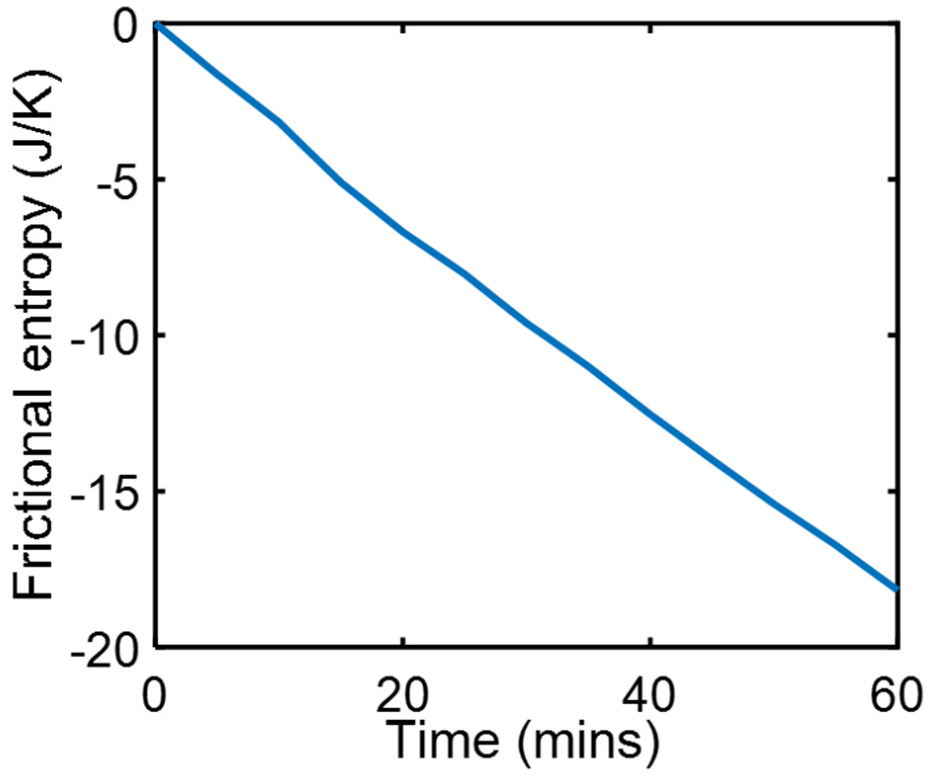
During a series of friction and wear tests, a copper rider pressed by 9.7 kg dead weight against a steel countersurface slid at steady speed $\dot{x}$ = 3.3 ms⁻¹ under carefully maintained thermal and lubricated boundary conditions [23]. Measured were friction force $F$ and temperatures at three locations in the copper, to estimate friction heat generation $F\dot{x}$, heat flow and surface temperature $T$, all of which were steady during sliding to render $\dot{T}=0$, which when substituted into Equation (18c) yields $S_{phen}^{\prime }=-{\int }_{t_o}^{t_f}\frac{F\dot{x}}{T}dt$. Using measured values, the integral was evaluated over the test time interval to obtain the entropy generation plot in Figure 1.

4.2. Mechanical Shearing of Grease—Shear Stress and Shear Strain (Helmholtz Potential)

0.25 kg of Aeroshell 14 aircraft NLGI 4 lithium grease in a cup was sheared by a rotating impeller. The grease-in-cup system was treated as closed and non-reacting. Tests and procedures [8] at impeller speed 3 Hz measured impeller power M_Tω (the product of torque M_T and rotational speed ω) and temperatures (via thermocouples) of grease T and ambient, which are plotted versus time in Figure 2a. In terms of native grease internal variables, $M_T\omega =V\tau \dot{\gamma }$ gives the shear power as the product of volume $V$, shear stress $\tau$ and shear strain rate $\dot{\gamma }$. Helmholtz entropy content density S_A—the first of Equations (14) divided by V—was substituted into Equation (18c) with ${\dot{N}}_k=0, Y=\tau$, $\dot{X}=V\dot{\gamma }$, to yield phenomenological entropy density

$$S_{phen}^{\prime }=-{\int }_{t_o}^{t_f}\frac{S_A\dot{T}}{T}dt-{\int }_{t_o}^{t_f}\frac{\tau \dot{\gamma }}{T}dt.$$

(21)

With the data of Figure 2a, the integrals in Equation (21) were estimated numerically via the methods of Section 1.2 to yield the entropy generation versus time plots in Figure 2b, where the MST entropy density and shear entropy density are the first and second integrals of Equation (21), respectively.

4.3. Discharge of Lithium-Ion Battery—Voltage and Charge (Helmholtz-Gibbs Coupling)

Four 3.7 V, 11.5 Ah single-cell lithium-ion batteries were discharged at a variable discharge current of 5 A and recharged at a constant current of 3 A [7]. Figure 3a plots voltage $v$, current I, temperatures of battery T and ambient, measured during the battery cycle. For a battery, the Helmholtz-Gibbs coupling, Section 2.7, yields $\sum {\mu }_k{\dot{N}}_k=vI$, the Ohmic power. Substituting into Equation (19c) yielded

$${{\dot{S}}^{\prime }}_{phen}=\frac{-S\dot{T}}{T}+\frac{vI}{T}.$$

(22)

Via the Gibbs-Duhem formulation, Equation (16), at constant pressure, $-S\dot{T}=q\dot{v}$ (applying Faraday’s electrolysis law, see paragraph after Equation (16)), substituted into Equation (22) and integrated over time rendered, for discharge and charge,

$$S_{phen}^{\prime }=\underset{t_o}{\overset{t_f}{\int }}\frac{q\dot{v}}{T}dt+\underset{t_o}{\overset{t_f}{\int }}\frac{vI}{T}dt.$$

(23)

Here, $q={\int }_{t_0}^{t_f}Idt$ is the charge content. With the data of Figure 3a, the integrals in Equation (23) were estimated via the methods of Section 1.2 to yield the entropy generation versus time plots in Figure 3b, where the ElectroChemicoThermal ECT entropy and Ohmic entropy are the first and second integrals of Equation (23), respectively.

4.4. Fatigue of Metals—Stress and Strain (Helmholtz Potential)

A high-resolution infra-red camera monitored the temperature profile of an SS 304 stainless steel rod subjected to a 10 Hz displacement-controlled cyclic bending load until fatigue failure [24]. See Figure 4a. Here, boundary work $Y\dot{X}=V\sigma :\dot{\epsilon }$, where $\sigma$ is the stress tensor and $\epsilon$ is the elemental strain rate tensor, both having elastic and plastic components, viz $\sigma ={\sigma }_e+{\sigma }_p$, $\epsilon ={\epsilon }_e+{\epsilon }_p$. Existing models [25] estimated the stress and strain. As in the case of grease shearing, Helmholtz entropy content density S_A—the first of Equations (14) divided by volume V—was substituted into (18c) with ${\dot{N}}_k=0$ to obtain

$$S_{phen}^{\prime }=-{\int }_{t_o}^{t_f}\frac{S_A\dot{T}}{T}dt-{\int }_{t_o}^{t_f}\frac{\sigma :\dot{\epsilon }}{T}dt.$$

(24)

Substituting stress, strain, temperature and material property values, the integrals in Equation (24) were estimated via the methods of Section 1.2 to render the entropy generation plots in Figure 4b, where the MST entropy density ${S^{\prime }}_{\mu T}$ (red plot) and load entropy density S’_W (blue plot) are the first and second integrals of Equation (24), respectively. For low-cycle fatigue, with significant plastic deformation, the modulus defined in Equations (12) and (13), substituted into entropy content density S_A in Equation (24), is the hardness modulus.

4.5. Pump Flow—Pressure and Flow Rate (Internal Energy)

Water flowed through a three-phase 15-hp 260-gpm centrifugal motor-pump, instrumented to measure inlet and exit pump pressures and flow rate [26], which are plotted versus time in Figure 5a. A valve adjusted the flow rate. Measured volumetric flow rate was converted to mass flow rate using the density of water ($\dot{m}=\rho \dot{V}$), and pump power $Y\dot{X}=M_T\omega$, the product of torque $M_T$ and rotational speed $\omega$. Substituting into Equation (19), with positive input power, yielded

$${{\dot{S}}^{\prime }}_{phen}=\frac{C_V\dot{T}}{T}+\frac{\sum \left[{\left(\dot{m}h\right)}_{exit}-{\left(\dot{m}h\right)}_{inlet}\right]}{T}+\frac{M_T\omega }{T}.$$

(25)

With no external heat source and assuming negligible rise in flow temperature which was not measured during this test—hence T is constant ambient temperature—the first right-side term in Equation (25) vanished. Integrating with respect to time,

$$S_{phen}^{\prime }=\underset{t_o}{\overset{t_f}{\int }}\frac{\sum \left[{\left(\dot{m}h\right)}_{exit}-{\left(\dot{m}h\right)}_{inlet}\right]}{T}dt+\underset{t_o}{\overset{t_f}{\int }}\frac{M_T\omega }{T}dt.$$

(26)

Substituting the data of Figure 5a, the integrals in Equation (26) yielded Figure 5b plots, where the flow entropy (measuring the change in the flow between inlet and exit, green plot) and load entropy (measuring the effect of power input into the pump, blue plot) are the first and second integrals of Equation (26), respectively.

5. Discussion

Here, reversible implies thermodynamic reversibility: any real system undergoing a spontaneous process cannot “revert” back to its original state without work from an external source, hence is thermodynamically irreversible. The reversible forms of Equations (9) (wherein $\delta S^{\prime }=0$) derived directly from Legendre transforms of entropy by Francois Massieu are called the Massieu functions [16,27]. Here, by using the irreversible form of internal energy change (Equation (5)), Equations (9) are termed the irreversible Massieu functions.

5.1. Phenomenology

In open thermal systems, $dS$ in the internal energy and enthalpy Equations (7) and (9a), including the heat and mass transfer entropies, is analogous to $SdT/T$ in the Helmholtz and Gibbs energy Equation (9a,b).

Comparing the entropy Equations (3) and (4) and the corresponding energy counterparts in Equations (5), (6) (8) and (9), via the state principle, showed that changes in entropy and energy between two states are path-independent, whether the process path is reversible or irreversible, i.e., $dS={dS}_{rev}={dS}_{irr}={\delta S}_{phen}-\delta S^{\prime }$; $dE={dE}_{rev}={dE}_{irr}={\delta E}_{phen}-T\delta S^{\prime }$, where E is any of internal energy U, enthalpy H, Helmholtz potential A or Gibbs potential G.

With a transformation representable along the linear and nonlinear paths, most thermodynamic characterizations employ energy change $dE={dE}_{rev}$ and entropy change $dS={dS}_{rev}$: only end state measurements of system variables (before and after process interaction) are required for evaluation; unlike $dE={dE}_{irr}={\delta E}_{phen}-T\delta S^{\prime }$ and $dS={dS}_{irr}={\delta S}_{phen}-\delta S^{\prime }$ which require instantaneous account of all active processes. Note that a system’s energy change dE and entropy change dS during a process can be negative or positive, depending on the direction of energy or entropy flow across system boundaries, hence neither dE nor dS measures the permanent changes in the system. On the other hand, entropy generation, Equations (1a), (7) and (9), evolves monotonically as stipulated by the second law. Figure 6 depicts the Phenomenological Entropy Generation theorem for a loaded or spontaneously transforming system. Equation (1b), which measures the entropy generated by the system’s internal irreversibilities alone, is in accordance with experience, appearing similar to the Gouy-Stodola theorem of availability (exergy) analysis [21,28,29,30]. Rearranging Equation (1b) renders another statement of the second law or entropy balance as

$$d{S}_{irr}={d\mathbb{S}}_{rev}={\delta \mathbb{S}}_{phen}-\delta S^{\prime },$$

(27)

which replaces entropy transfer in Prigogine’s entropy balance, Equation (3), with phenomenological entropy, from which entropy generation is subtracted.

As discussed previously, the quasi-reversible terms in the foregoing formulations proceed at constant, often standardized or predetermined rates for a given transformation, making them negligible in instantaneous energy dissipation/degradation monitoring for which the phenomenological terms are used.

Table 1. Summary of entropy generation formulations for various system categories, with examples. Here, subscript e, and superscripts r, p and d represent flow, reactants, products and diffusion, respectively. For thermal systems, $\mu$ is the molar enthalpy $\frac{\partial H}{\partial N}$. For other (chemical, etc.) reactive/energy systems, $\mu$ is the molar Gibbs energy or chemical potential $\frac{\partial G}{\partial N}$. More information on $c$, $\beta$ and $\lambda$ is in Section 2.5 and Appendix A.

Category	Phenomenological Entropy Generation ${\mathit{\delta }\mathbb{S}}_{\mathit{p}\mathit{h}\mathit{e}\mathit{n}}$	Example
Open Internal Energy	${\delta \mathbb{S}}_{U,phen}=$ $\frac{C_{X}dT}{T}+\frac{\left(u+Pv\right) {dN}_e}{T}-\frac{\sum Y_{l}d{X}_l }{T}$ Equation (10a) (for a non-reacting system)	Compressor (with temperature rise and boundary work):
		${\dot{\mathbb{S}}}_{U,phen}=\frac{C_V\dot{T}}{T}+\frac{\sum \left[{\left({\dot{N}}_{e}h\right)}_{exit}-{\left({\dot{N}}_{e}h\right)}_{inlet}\right]}{T}-\frac{Y\dot{X}}{T}$ (Rate form in Equation (19))
Thermal Enthalpy	${\delta \mathbb{S}}_{H,phen}=$ $\frac{C_{Y}dT}{T}+\frac{\sum X_{l}d{Y}_l }{T}+\frac{\sum {\mu }_{k}d{N}_k}{T}$ Equation (10b) (for a closed system)	Combustion systems without boundary work:
		${\delta \mathbb{S}}_{H,phen}=\frac{C_{p}dT}{T}+\frac{\sum {\mu }_k{{dN}^r}_k}{T}-\frac{\sum {\mu }_k{{dN}^p}_k}{T}$
Boundary-Loaded Helmholtz potential	${\delta \mathbb{S}}_{A,phen}=$ $\frac{-S_{A}dT}{T}-\frac{\sum Y_{l}d{X}_l }{T}+\frac{\sum {\mu }_{k}d{N}_k}{T}$ Equation (10c)	Mechanical loading, e.g., shearing without oxidation:
		${\delta \mathbb{S}}_{A,phen}=-\left(\rho c_{\gamma }lnT+\beta \gamma \right)\frac{dT}{T}-\frac{\tau d\gamma }{T}$
Reactive/Energy Gibbs potential	${\delta \mathbb{S}}_{G,phen}=$ $\frac{-S_{G}dT}{T}+\frac{\sum X_{l}d{Y}_l }{T}+\frac{\sum {\mu }_k{\dot{N}}_k}{T}$ Equation (10d)	Electrochemical energy systems, e.g., batteries:
		${\delta \mathbb{S}}_{G,phen}=-\left(ClnT-{\lambda }_{Y}q\right)\frac{dT}{T}+\frac{\sum {\mu }_k{{dN}^r}_k}{T}-\frac{\sum {\mu }_k{{dN}^p}_k}{T}+\frac{\sum {\mu }_k{{dN}^d}_k}{T}$
		Via Gibbs-Helmholtz coupling:
		${\delta \mathbb{S}}_{phen}=-\left(ClnT-{\lambda }_{X}q\right)\frac{dT}{T}+\frac{vdq}{T}$
		Via Gibbs-Duhem formulation:
		${\delta \mathbb{S}}_{phen}=\frac{-qdv}{T}+\frac{vdq}{T}$

summarizes phenomenological entropy generations derived in this article for various classes of open and closed systems.

5.2. Steady vs. Unsteady Systems: Minimum Entropy Generation (MEG) vs. MicroStructuroThermal (MST) Entropy

According to Onsager and Prigogine, the minimum entropy generation rate for a system to exist (minimally active) is the quotient of its primary work interaction (or energy transfer) and boundary temperature, i.e., ${{\dot{S}}^{\prime }}_{min}=\frac{Y\dot{X}}{T}$ [5,6,12,13]. The minimum entropy generation rates for internally reactive non-thermal open systems, including terms that characterize every significant interaction, can be derived from Equations (18a) and (19). For systems with boundary-deforming external loads, minimum entropy generation rate

$${{\dot{S}}^{\prime }}_{min}=\frac{\sum \left[{\left({\dot{N}}_{e}h\right)}_{exit}-{\left({\dot{N}}_{e}h\right)}_{inlet}\right]}{T}-\frac{Y\dot{X}}{T}+\frac{\sum {\mu }_k{\dot{N}}_k}{T},$$

(28a)

and from (18b), for open systems without boundary-deforming work,

$${{\dot{S}}^{\prime }}_{min}=\frac{\sum \left[{\left({\dot{N}}_{e}h\right)}_{exit}-{\left({\dot{N}}_{e}h\right)}_{inlet}\right]}{T}+\frac{X\dot{Y}}{T}+\frac{\sum {\mu }_k{\dot{N}}_k}{T}.$$

(28b)

Equations (28) only apply to steady interactions where temperature is controlled or assumed to be constant (dT ≈ 0). Equations (28) present the minimum conditions for simultaneous real interactions to occur (i.e., minimum perturbation from equilibrium). The steady-state frictional wear in Section 4.1 demonstrates minimum entropy generation.

For unsteady anisothermal interactions, often encountered in uncontrolled non-thermal systems (electronic, structural, mechanical, chemical, etc.), the free energies introduced the afore-named MicroStructuroThermal (MST) entropy

$${{\dot{S}}^{\prime }}_{\mu T}=\frac{-S\dot{T}}{T}.$$

(29)

The MST entropy of Equation (29) accompanies the primary interactions defined by Minimum Entropy Generation (MEG) in Equations (28). This accords with the thermodynamic state postulate [12,16,31] which requires r + 1 independent, intensive properties to fully specify the state of a simple system undergoing r primary work interactions. In non-thermal systems, the MST entropy measures the effects of energy dissipated as heat in the system, which is therefore unavailable for work. As such, the MST entropy must be minimized to decelerate degradation of non-thermal systems, the limit of which is the MEG (where ${{\dot{S}}^{\prime }}_{\mu T}=0$). Figure 7 depicts minimum entropy generation, a slight/minimal deviation from reversibility.

In the sample demonstrations in Figure 3b and Figure 4b, the ECT/MST entropy (red plots) is significantly lower than the primary interaction entropy or MEG (blue plots), which may have justified prior approaches neglecting the former via an order of magnitude analysis. However, recent works [7,8,9,10] have shown that the ECT/MST entropy, measuring the free energy dissipation, contributes significantly to degradation.

5.3. Dissipation Factor and Entropic Efficiency

To measure a non-thermal system’s dissipation tendencies relative to useful work output, define the dissipation factor

$$J=\frac{{S^{\prime }}_{\mu T}}{{S^{\prime }}_W+{S^{\prime }}_N},$$

(30)

the ratio of the MicroStructuroThermal MST entropy ${S^{\prime }}_{\mu T}$ to the sum of boundary work ${S^{\prime }}_W$ and compositional change ${S^{\prime }}_N$ entropies, which can consistently characterize system response to dissipative mechanisms as well as multiple systems undergoing the same output/input work. A low J (minimal dissipation relative to available work) is desired for optimum performance and durability.

An examination of entropy Equations (7) and (9) indicates that low entropy generation ($\delta S^{\prime }\to 0$) would make more useful system energy available, the limit of which is the reversible system ($\delta S^{\prime }=0$). Define entropic efficiency

$${\eta }_{S^{\prime }}=\frac{{S^{\prime }}_W+{S^{\prime }}_N}{S_{rev}},$$

(31)

the ratio of the sum of boundary work and compositional change entropies to reversible entropy $S_{rev}$. With an ideal (reversible or perfect) system—for which ${S^{\prime }}_W+{S^{\prime }}_N=S_{rev}$—establishing 100% efficiency, a high ${\eta }_{S^{\prime }}$ is preferred for slow degradation and optimum performance. Equation (31) appears similar to the exergy-based second-law efficiency which uses reversible work and boundary work at end states (i.e., not instantaneously determined during process interaction) [31,32].

5.4. Thermal vs. Non-Thermal Systems—Internal Energy and Enthalpy vs. the Free Energies

Internal energy- and enthalpy-based entropy generations, Equations (7) and (9a), have an entropy change term $dS$, which includes heat transfer entropy, accentuating the already known suitability and convenience of internal energy and enthalpy (heat content) in characterizing primarily heat-based (or thermal) systems. The Helmholtz- and Gibbs-based entropies of Equation (9b,c) encapsulate the effects of entropy transfers in the observable evolution of the system’s internal variables (material properties and temperature). This makes the free energies and the consequent “free entropies” particularly convenient for non-thermal systems and interactions where heat transfer is not readily measurable and for which thermal mechanisms primarily emanate from energy dissipation. The free entropies are more consistent for assessing system transformations from observable and measurable system variables, irrespective of surrounding conditions.

Significant increase in temperature reduces available free energy via the MicroStructuroThermal MST term, see Equation (8b,c). For non-thermal (mechanical, structural, chemical, electronic, magnetic, electrical, etc.) systems, this accords with experience, further making the free entropy formulations derived from the free energies suitable for non-thermal system characterizations. Thermal systems are utilized for heat content and typically have high temperature increase rate. This indicates that a high MST component—which accompanies high thermal energy—is favorable for thermal systems. Hence, the free energies are subject to misinterpretation and not recommended for characterizing thermal systems.

6. Summary and Conclusions

Building on the first-principles foundations of modern irreversible thermodynamics laid by Clausius, Rayleigh, Onsager and Prigogine, this article formulated universally consistent, instantaneous entropy generations for diverse macroscopic system categories (see summary in Table 1). Presented was thermodynamic resolution of the active processes and unsteady system responses during loading using readily evaluated entropy generation. A Phenomenological Entropy Generation (PEG) theorem was derived and proposed, expounding the significances of the newly introduced MicroStructuroThermal MST entropy (or ElectroChemicoThermal ECT entropy for electrochemical power systems) and previously neglected reversible entropy to characteristic entropy generation. Extending and generalizing Gibbs theory of thermodynamic stability, the Clausius inequality, Rayleigh’s energy dissipation principle, Onsager’s reciprocity, and Prigogine’s entropy balance—the hallmarks of classical and modern irreversible thermodynamics [4,5,6,12,13,33]—this article, using results from recently published experimental works [7,8,9,10], demonstrated that:

• a combination of the thermodynamic potentials and the irreversible form of the TdS equation yields the irreversible Massieu functions;
• steady-state systems generate entropy at a minimum rate which, for a boundary-loaded, internally reactive open system, is the sum of boundary work/load entropy ${S^{\prime }}_W$ and compositional change entropy ${S^{\prime }}_N$ rates;
• for unsteady non-thermal systems, a microstructurothermal MST entropy is included to characterize the accompanying instantaneous transients during system transformation;
• phenomenological entropy generation ${S^{\prime }}_{phen}$ is the sum of boundary work/load entropy ${S^{\prime }}_W$, compositional change entropy ${S^{\prime }}_N$ and microstructurothermal MST entropy ${S^{\prime }}_{\mu T}$ (ElectroChemicoThermal ECT entropy ${S^{\prime }}_{VT}$ for electrochemical systems);
• entropy generation is the difference between phenomenological ${S^{\prime }}_{phen}$ and reversible $S_{rev}$ entropies at every instant, named the Phenomenological Entropy Generation (PEG) Theorem;
• along the phenomenological path, thermodynamic and other states germane to evaluating ${S^{\prime }}_{phen}$ and $S_{rev}$ are observable (measurable), permitting evaluation of entropy generation $\delta S^{\prime }$;
• entropy generation is always non-negative in accordance with the second law, while its constituent terms ${S^{\prime }}_{phen}$ and $S_{rev}$ are directional, negative for a loaded system and positive for an energized system. This implies $\left|{S^{\prime }}_{phen}\right|\le \left|S_{rev}\right|$ during load application/work output or active species decomposition, and $\left|{S^{\prime }}_{phen}\right|\ge \left|S_{rev}\right|$ during energization/work input or active species formation, in accordance with experience and thermodynamic laws. In plain words, measurable energy obtained from a real system is always less than the theoretical maximum/reversible energy, and measurable energy added to a real system is always more than the minimum/reversible energy. (Modulus signs indicate magnitudes only).

References

- Clapeyron, B.E. Memoir sur la puissance motrice de la chaleur. J. De L’école R. Polytech. 1834, 23, 153–190. [Google Scholar]
- Massieu, F. Sur les Fonctions caractéristiques des divers fluides. CR Acad. Sci. Paris 1869, 69, 858–862. [Google Scholar]
- Rayleigh, J.W.S.B. The Theory of Sound; Macmillan: New York, NY, USA, 1896; Volume 2. [Google Scholar]
- Onsager, L. Reciprocal Relations in Irreversible Processes. Phys. Rev. 1931, 37, 183–196. [Google Scholar] [CrossRef]
- Prigogine, I. Introduction to Thermodynamics of Irreversible Processes; Thomas, C.C., Ed.; Cambridge University Press: Cambridge, UK, 1955. [Google Scholar]
- de Groot, S.R.; Mazur, P. Non-Equilibrium Thermodynamics; Dover Publications Inc.: New York, NY, USA, 2011. [Google Scholar]
- Osara, J.; Bryant, M. A Thermodynamic Model for Lithium-Ion Battery Degradation: Application of the Degradation-Entropy Generation Theorem. Inventions 2019, 4, 23. [Google Scholar] [CrossRef]
- Osara, J.A.; Bryant, M.D. Thermodynamics of grease degradation. Tribol. Int. 2019, 137, 433–445. [Google Scholar] [CrossRef]
- Osara, J.A.; Bryant, M.D. Thermodynamics of fatigue: Degradation-entropy generation methodology for system and process characterization and failure analysis. Entropy 2019, 21, 685. [Google Scholar] [CrossRef]
- Osara, J.A.; Bryant, M.D. Thermodynamics of Lead-Acid Battery Degradation: Application of the Degradation-Entropy Generation Methodology. J. Electrochem. Soc. 2019, 166, A4188–A4210. [Google Scholar] [CrossRef]
- Bryant, M.D.; Khonsari, M.M.; Ling, F.F. On the thermodynamics of degradation. Proc. R. Soc. A Math. Phys. Eng. Sci. 2008, 464, 2001–2014. [Google Scholar] [CrossRef]
- Kondepudi, D.; Prigogine, I. Modern Thermodynamics: From Heat Engines to Dissipative Structures; John Wiley & Sons Ltd.: Hoboken, NJ, USA, 1998. [Google Scholar]
- de Groot, S.R. Thermodynamics of Irreversible Processes; North-Holland Publishing Company: Amsterdam, The Netherlands, 1951. [Google Scholar] [CrossRef]
- Taub, H.; Schilling, D.L. Principles of Communication Systems; McGraw-Hill: New York, NY, USA, 1971. [Google Scholar]
- Muschik, W. Fundamentals of Non-Equilibrium Thermodynamics. In Non-Equilibrium Thermodynamics with Applications to Solids; Muschik, W., Ed.; Springer: Berlin/Heidelberg, Germany, 1993; pp. 1–67. [Google Scholar]
- Callen, H.B. Thermodynamics and An Introduction to Thermostatistics; John Wiley & Sons, Ltd.: Hoboken, NJ, USA, 1985. [Google Scholar]
- Gibbs, J.W. The Collected Works of J. Willard Gibbs...: Thermodynamics; Longmans, Green and Company: London, UK, 1928; Volume 1. [Google Scholar]
- Pauli, W. Thermodynamics and The Kinetic Theory of Gases; Pauli Lectures on Physics Vol 3 Dover Books; Courier Corporation: Honolulu, HI, USA, 1973. [Google Scholar]
- Osara, J.A. Thermodynamics of manufacturing processes—The workpiece and the machinery. Inventions 2019, 4, 28. [Google Scholar] [CrossRef]
- Bove, R.; Ubertini, S. (Eds.) Modeling Solid Oxide Fuel Cells Methods, Procedures and Techniques; Spinger: Berlin/Heidelberg, Germany, 2008. [Google Scholar]
- Bejan, A. Advanced Engineering Thermodynamics, 3rd ed.; John Wiley & Sons, Inc.: Hoboken, NJ, USA, 2006. [Google Scholar] [CrossRef]
- Osara, J.A.; Chatra, S.; Lugt, P.M. Grease Material Properties from First Principles Thermodynamics. Lubr. Sci. 2023, 36, 36–50. [Google Scholar] [CrossRef]
- Doelling, K.L.; Ling, F.F.; Bryant, M.D.; Heilman, B.P. An Experimental Study on the Correlation between Wear and Entropy Flow in Machinery Components. J. Appl. Phys. 2000, 88, 2999–3003. [Google Scholar] [CrossRef]
- Naderi, M.; Khonsari, M.M. An experimental approach to low-cycle fatigue damage based on thermodynamic entropy. Int. J. Solids Struct. 2010, 47, 875–880. [Google Scholar] [CrossRef]
- Morrow, J.D. Cyclic Plastic Strain Energy and Fatigue of Metals. In Internal Friction, Damping, and Cyclic Plasticity; ASTM International: West Conshohocken, PA, USA, 1965. [Google Scholar]
- Rincon, J.; Osara, J.A.; Bryant, M.D.; Fernandez, B. Shannon’s Machine Capacity & Degradation-Entropy Generation Methodologies for Failure Detection: Practical Applications to Motor-Pump Systems; Turbomachinery & Pump Symposia: Houston, TX, USA, 2021. [Google Scholar]
- Balian, R. François Massieu and the thermodynamic potentials. Comptes Rendus Phys. 2017, 18, 526–530. [Google Scholar] [CrossRef]
- Burghardt, M.D.; Harbach, J.A. Engineering Thermodynamics, 4th ed.; HarperCollinsCollege Publishers: New York, NY, USA, 1993. [Google Scholar]
- Bejan, A. The Method of Entropy Generation Minimization. In Energy and the Environment; Sage Publications: Thousand Oaks, CA, USA, 1990; pp. 11–22. [Google Scholar]
- Pal, R. Demystification of the Gouy-Stodola theorem of thermodynamics for closed systems. Int. J. Mech. Eng. Educ. 2017, 45, 142–153. [Google Scholar] [CrossRef]
- Moran, M.J.; Shapiro, H.N. Fundamentals of Engineering Thermodynamics, 5th ed.; Wiley: Hoboken, NJ, USA, 2004. [Google Scholar]
- Çengel, Y.A.; Boles, M.A. Thermodynamics—An Engineering Approach; McGraw-Hill Education: New York, NY, USA, 2015. [Google Scholar]
- Nicolis, G.; Prigogine, I. Self-Organization in Nonequilibrium Systems; John Wiley & Sons Inc.: New York, NY, USA, 1977. [Google Scholar]
Figure 1.
Phenomenological frictional entropy over time during boundary-lubricated frictional wear.
Figure 2.
(a) Monitored parameters during grease shearing and (b) phenomenological entropy density terms: shear entropy density and MST entropy density over time [8].
Figure 3.
(a) Monitored parameters during Li-ion battery cycling showing 1.5 h discharge starting at ~5 A, followed by 1.5 h charge at 3 A. (b) phenomenological entropy terms: Ohmic entropy and ECT entropy over time [7].
Figure 4.
(a) Monitored parameters during steel rod fatigue loading and (b) phenomenological entropy terms: load entropy density and MST entropy density over time [9].
Figure 5.
(a) Monitored inlet/exit pressures and flow rate during a centrifugal motor pump operation, and (b) phenomenological entropy terms: flow entropy and load entropy over time.
Figure 6.
Illustrations of the Phenomenological Entropy Generation theorem, showing reversible (green) and phenomenological (purple) paths; the vertical difference between the paths (see black arrows) defines entropy generation or energy dissipation (orange). (a) Rates and (b) Accumulations .
Figure 7.
Illustrations of the Minimum Entropy Generation theorem, showing reversible (green) and minimum (purple) paths; the difference between the paths defines minimum entropy generation (orange). (a) Rates and (b) Accumulations .