
Mechanisms for Robust Local Differential Privacy

Faculty of Electrical Engineering, Mathematics and Computer Science, University of Twente, 7522 NB Enschede, The Netherlands
*
Authors to whom correspondence should be addressed.
Entropy 2024, 26(3), 233; https://doi.org/10.3390/e26030233
Submission received: 11 January 2024
/
Revised: 29 February 2024
/
Accepted: 3 March 2024
/
Published: 6 March 2024
(This article belongs to the Special Issue Information Theory for Distributed Systems)
Abstract
:We consider privacy mechanisms for releasing data , where S is sensitive and U is non-sensitive. We introduce the robust local differential privacy (RLDP) framework, which provides strong privacy guarantees, while preserving utility. This is achieved by providing robust privacy: our mechanisms do not only provide privacy with respect to a publicly available estimate of the unknown true distribution, but also with respect to similar distributions. Such robustness mitigates the potential privacy leaks that might arise from the difference between the true distribution and the estimated one. At the same time, we mitigate the utility penalties that come with ordinary differential privacy, which involves making worst-case assumptions and dealing with extreme cases. We achieve robustness in privacy by constructing an uncertainty set based on a Rényi divergence. By analyzing the structure of this set and approximating it with a polytope, we can use robust optimization to find mechanisms with high utility. However, this relies on vertex enumeration and becomes computationally inaccessible for large input spaces. Therefore, we also introduce two low-complexity algorithms that build on existing LDP mechanisms. We evaluate the utility and robustness of the mechanisms using numerical experiments and demonstrate that our mechanisms provide robust privacy, while achieving a utility that is close to optimal.
1. Introduction
We consider the setting in which an aggregator collects data from many users with the purpose of, for instance, computing statistics or training a machine learning model. In particular, the data contain sensitive information and users do not trust the aggregator. Therefore, they employ a privacy mechanism that transforms the data before sending it to the aggregator. Users have data from a finite alphabet , where is sensitive information and is non-sensitive. Data are distributed i.i.d. across users according to the distribution . In order to preserve their privacy, users disclose a sanitized version Y of X by using a privacy mechanism . The aim is that Y contains as much information about X as possible without leaking too much information about S. The challenge that is addressed in this paper is to develop good privacy mechanisms. This scenario and closely related ones were studied in, for instance [1,2,3,4,5,6,7,8,9,10,11]. In this paper, we use the following version of local differential privacy (LDP), as introduced in [3]:
for all and privacy parameter . In addition, we measure the utility of Y through the mutual information . We discuss differences with related work in Section 2.
Note that if all information is sensitive, i.e., if , (1) reduces to
which is the traditional LDP constraint [1,2,5]. An important property of (2) is that it does not depend on , but only on . The independence of is a key factor in the success of differential privacy, since it leverages the need to make assumptions about the distribution of the data or on the background/side-knowledge available to the aggregator. As is clear from (1), however, independence from no longer holds if not all data are sensitive.
Assuming that is known, one can develop good privacy mechanisms for various settings with partially sensitive information [3,6,12]. In practice, however, has to be modeled using domain knowledge or estimated from data, leading to errors. The prevalent approach in the literature has been to develop privacy mechanisms based on a (point) estimate and analyze sensitivity with respect to. errors in this estimate. In this work, we follow the approach that was proposed in [13,14], which is to construct a set of probability distributions that we are confident contains . Subsequently, we construct privacy mechanisms that aim to maximize utility, while satisfying (1) for all probability distributions in . We call the resulting privacy framework robust local differential privacy (RLDP).
In a sense, RLDP is a relaxed form of privacy. Indeed, it may seem appealing, but it is—as we illustrate next—often infeasible to enforce (1) for all possible distributions. To this end, we consider two extreme cases. First, consider a joint distribution of S and U under which . Intuitively, we cannot disclose much information about U, since this is directly leaking information about S. As such, the utility of Y is low. Next, consider a joint distribution under which S and U are independent. Intuitively, we can disclose U without additional precautions, providing a high utility on Y. The point is that we need to design a single privacy mechanism that satisfies (1) for all distributions, including the ‘worst case’ in which , leading to low utility Y. In this work, we take the mid-ground between, on the one hand, only using a point estimate and, on the other hand, using all possible distributions. We do so by defining a set of ‘reasonable’ distributions . In particular, we construct based on public side-information. This public side information consists of n pairs of data , which like the data of users are i.i.d. according to unknown distribution . Our set is constructed as a closed ball under a Rényi divergence around the maximum likelihood point estimate of . By doing so, we are (statistically) confident that contains , with the radius of the ball controlling the confidence level.
The RLDP framework is an instance of the more general Pufferfish framework [15]. In Section 2, we make this connection explicit and use it to describe the semantic privacy guarantees that are offered by RLDP.
The main contributions of this paper are as follows:
- We use a Rényi divergence to construct and analyze the resulting structure and statistics of . In particular, we demonstrate that projections of are again balls under the same divergence. Moreover, we bound the projected sets in terms of an norm.
- A drawback of this method is that it relies on vertex enumeration and is, therefore, computationally unfeasible for large alphabets. Therefore, we introduce two low-complexity privacy mechanisms. The first is independent reporting (IR), in which S and U are reported through separate LDP mechanisms.
- We characterize the conditions that underlying LDP mechanisms have to satisfy in order for IR to ensure RLDP. Furthermore, while IR can incorporate any LDP mechanism, we show that it is optimal to use randomized response [19]. This drastically reduces the search space and allows us to find the optimal IR mechanism using low-dimensional optimization.
- The second low-complexity mechanism that we develop is called secret-randomized response (SRR) and is based on randomized response.
- We show that SRR maximizes mutual information in the low-privacy regime for the case that is the entire probability simplex.
- We demonstrate the improved utility of RLDP over LDP with numerical experiments. In particular, we compare the performance of our mechanisms with generalized random response [5]. We provide results for both synthetic data sets and real-world census data.
The structure of this paper is as follows: After discussing related work in Section 2, we describe the model in detail in Section 3. In Section 4, we present results on the structure and statistics of projections of . These results are used in Section 5 to develop the PolyOpt privacy mechanism. Low-complexity privacy mechanisms are presented in Section 6 and Section 7. In Section 8, we evaluate the discussed methods experimentally. Finally, in Section 9, we provide a discussion of our results and provide an outlook on future work. Most proofs are deferred to Appendix A.
2. Related Work
2.1. The Pufferfish Framework
Our RLDP framework is an instance of the more general Pufferfish framework [15]. In this subsection, we make this connection explicit and elaborate on the semantic guarantees offered by RLDP.
A privacy definition following the Pufferfish framework specifies (i) a set of potential secrets, (ii) a set of discriminative pairs of secrets, and (iii) a set of assumptions about how data are generated. In RLDP the potential secrets are the possible values of S, i.e., . We want to prevent the aggregator from learning anything about S. This means that it should not be able to distinguish the case from for all , so all non-identical pairs are discriminative. Note that this relies on being finite, with extensions to continuous discussed in detail in [15].
The set of assumptions on how data are generated consist, in our setting, of probability distributions over . A key idea in Pufferfish is that this set explicitly models the information that is available to an attacker, i.e., an entity that is trying to infer information about S by observing Y. In our setting, the aggregator is the only attacker and a probability distribution P over captures the beliefs that the attacker has about S prior to seeing Y. We can rewrite (1) as
and see that our local differential privacy constraint (1) can be interpreted as the condition that the posterior distribution of S after seeing Y must be very close to the prior distribution. The relevance of P is that it captures a specific set of beliefs of the attacker. As such, we want (3) to hold for various values of P, where each P captures specific background/side-knowledge available to the attacker/aggregator. Note that by doing so we are not making any claims about the actual knowledge available to the aggregator, but instead describing the possible scenarios for which we want to protect the privacy of users. In Pufferfish, these possible scenarios are called the set of assumptions on how data are generated, and in RLDP this is .
Often, side-information in the form of domain knowledge or existing data is publicly available; i.e., to both the users and the aggregator. This public side-information may suggest, for instance, that there is, at most, limited dependence between S and U. In that case, protecting against attackers who have the belief that incurs an enormous penalty in achieved utility. It is true that those attackers gain a lot of information on S by observing Y. However, they could have also obtained this information from the public side-information directly. Therefore, the approach taken in the Pufferfish framework and in this paper is that we only protect against attackers that have beliefs, i.e., distributions P, that are in line with publicly available side information.
A challenge in working with the Pufferfish framework is that it is often challenging to find good mechanisms. A general mechanism is proposed in [20], but it relies on enumerating over all distributions in , which is an uncountable set in our setting and cannot be used here. A constrained version of Pufferfish that facilitates analysis and a methodology for finding good mechanisms is proposed in [21]. Another interesting line of work is to model correlations between users in the non-local differential privacy setting [22]. Finally, ref. [23] proposed a modeling framework for capturing domain knowledge about the data. In contrast, in the current work, we impose constraints that are learned from data. Our setting does not fit any of the frameworks for which good mechanisms are known in the literature. One of the main contributions of this paper is to develop such mechanisms.
2.2. Other Privacy Frameworks
Disclosing X through a privacy mechanism that protects sensitive information S has been studied extensively. One line of work starts from differential privacy [24] and imposes the additional challenge that the aggregator cannot be trusted, leading to the concept of local differential privacy [1,2,5]. For this setting, several privacy mechanisms exist, including randomized response [19] and unary encoding [25]. Optimal LDP mechanisms under a variety of utility metrics, including mutual information, are found in [5]. In [1,2,5], all data are sensitive, i.e., . The variation of LDP for the case of disclosing , where only S is sensitive, was proposed in [3] and is the setting that we study in this paper. Another line of work connects this setting to the information bottleneck [26], leading to a privacy constraint in terms of mutual information [6,8,9,10]. In these works, it is shown that approaches to optimizing the information bottleneck also work for finding good privacy mechanisms.
Next to differential privacy and mutual information as privacy measures, a multitude of other privacy frameworks and leakage measures exist [27]. Some of these have been studied in the context of privacy mechanisms. In [7,11], privacy leakage is measured through the improved potential of statistical inference by an attacker after seeing the disclosed information. This measure is formulated through a general cost function, with mutual information resulting as a special case. Perfect privacy, which demands the output to be independent of the sensitive data, was studied in [28], and methods were given to find optimal mechanisms in this setting. An estimation-theoretic framework was studied in [29,30]. Our use of a Rényi divergence in the construction of may suggest considering a generalization of our privacy definition. This could be achieved by considering, for instance, a Rényi divergence in the privacy constraint, as done in [31]. Along a different line, in [32], the maximal leakage measure with a clear operational interpretation is defined. In [33], this measure is generalized to a parametrized measure, enabling interpolating between maximal leakage and mutual information. A stronger, pointwise, version of the maximal leakage measure is proposed in [34]. These are interesting research directions but not pursued in this paper.
Our setting is a special case of a Markov chain , where only X is observed. This Markov chain is typically studied in the information bottleneck and privacy funnel settings [6,26]. We do not generalize to this setting, because we need observations of S for the estimate of . Without direct observations of s, we can only make worst-case assumptions on , leading to very poor utility. A different type of model, in which only part of the information in X is sensitive, is proposed in [12]. This is a block-structured model in which X is partitioned and information about the partition of an element is sensitive but its index in the partition is not. Our setting of does not fit this model. One can partition according to , but our privacy constraints are different from [12]. We will elaborate on this in Section 6.
2.3. Robustness
The distribution is not available in practice. The approach taken in most works is to estimate from data and analyze sensitivity with respect to this estimate . One of the contributions in [7] is to quantify the impact of mismatched priors, i.e., the impact of not knowing exactly. A bound on the resulting level of privacy is derived in terms of the total variational distance between the actual and the estimated . The setting in [35] is similar to ours: A ball of probability distributions, centered around a point estimate, was defined that contains with high probability. It was then shown that a privacy mechanism that was designed based on the empirical distribution was valid for the entire set for a looser privacy constraint. The privacy slack was quantified and shown to approach zero as the size of the data set increased. An important difference with the current work was that we explicitly optimize the privacy mechanism over the uncertainty set. Another difference is that we base our ball on a Rényi divergence, whereas [35] used an norm. The main technical tool used in [35] was large deviations theory, whereas we rely on convex analysis and robust optimization. We also mention [36,37]. In [36] it is assumed that nothing is known about and . It is shown that good privacy mechanisms can be found through a connection to maximal correlation, see also [38]. In [37], sets of probability distributions are not derived from data but carefully modeled such that optimal mechanisms can be derived analytically.
Using robust optimization [16] to find a good mechanism that satisfies privacy constraints for all in uncertainty set was proposed in [13,14]. In this work, we generalize and extend results from [14]. The idea of robust optimization is that constraints in an optimization problem contain uncertain parameters that are known to come from a (a priori defined) uncertainty set. The constraints must hold for possible values of the uncertain parameters. A key result is that, using Fenchel duality, the problem can be expressed in terms of the support function of the uncertainty set and the convex conjugate of the constraint [16,17]. The case where the uncertain parameters are probabilities is known as distributionally robust optimization. Using results from [39], it was shown in [40] how an uncertainty set can be constructed from data using an f-divergence, providing an approximate confidence set. Confidence sets for parameters that are not necessarily probabilities were constructed in [18] under a -divergence. Convergence of robust optimization based on f-divergences was studied in [41] and for the case of a KL-divergence in [42]. In [43], it is shown how distributionally robust optimization problems over Wasserstein balls can be reformulated as convex problems. For the regular differential privacy setting, distributionally robust optimization was used in [44] to find optimal additive privacy mechanisms for a general perturbation cost function. In this paper, we show how robust optimization can be applied to the setting of partially sensitive information with local differential privacy.
2.4. Miscellaneous
Another line of work on privacy mechanisms builds on recent advances in generative adversarial networks [45]. In [46,47], a generative adversarial framework is used to provide privacy mechanisms that do not use explicit expressions for . Even though this is not explicitly addressed in [46,47], it is expected that the generalization properties of networks will provide a form of robustness. Closely related approaches are used in the field of face recognition [48,49], with the aim of preventing biometric profiling [50]. The leakage measures that are used in [48,49], however, do not seem to have an operational interpretation.
Disclosing information in a privacy-preserving way is one of the main challenges in official statistics [51,52]. The setting considered in the current paper is closely connected to disclosing a table with microdata, where each record in the table is released independently of the other records. This approach to disclosing microdata was studied in [4] by considering expected error as the utility measure and mutual information as the privacy measure. The resulting optimization problem corresponds to the traditional rate-distortion problem.
3. Model and Preliminaries
In this section, we give an overview of the setting and objectives of this paper. The notation used in this section, as well as the rest of the paper, is summarized in Table 1.
The data space is , where and are finite sets. We write , , and . Data items are drawn from a probability distribution in , the space of probability distributions on ; here, S represents sensitive data, while U represents non-sensitive data. The aggregator’s aim is to create a privacy mechanism such that contains as much information about X as possible, while not leaking too much information about S.
The mechanism is a probabilistic map, which we represent by a left stochastic matrix , and we write . Often, we identify , and likewise for other sets.
The distribution is not known exactly. Instead, there is a set of possible distributions , where denotes the probability simplex over . We choose in such a way that it is likely that . The uncertainty set captures our uncertainty about , we guarantee privacy for all . We denote this as robust local differential privacy (RLDP).
Definition 1
(Robust Local Differential Privacy). Let and . We say that satisfies -RLDP if for all , all , and all we have
Note that we use the notation to emphasize that X is distributed according to P. If no confusion can arise, we often leave out the subscript , to improve readability. Note that we can also write
so Definition 1 depends on the conditional probabilities of U given and . It does not, however, depend on the realization of U.
For clarity and use in future sections, we give the definition of regular LDP [1], which is used when the goal is to obfuscate all of X, rather than just S.
Definition 2
(Local Differential Privacy). Let . We say that satisfies ε-LDP if for all and all we have
Now, for aggregator uncertainty about , as captured by , we suppose there is a data base accessible to the user, where each is drawn independently from . Based on this, the user produces an estimate of . In the experiments, we consider a maximum likelihood estimator, i.e., . We construct the uncertainty set as a closed ball around . In particular, let be the Rényi divergence of order on , i.e., for
The case follows, in fact, as a limit from the case. Similarly, the definition can be extended to by taking the corresponding limits, but in this paper we restrict our attention to to keep the presentation clear. Note that , the Kullback–Leibler divergence, and , where the -divergence is . In general, a Rényi divergence is a continuous increasing function of a power divergence (a.k.a. Hellinger divergence) [39,53,54], an example of an f-divergence. We omit from the notation when it is clear from the context.
We define by fixing a bound and letting
Since a Rényi divergence is a continuous increasing function of an f-divergence, it follows from [39,40] that is a confidence set for . In particular, for the case of , which will be used in our numerical experiments in Section 8, for suitable B, we have
with , where is the cumulative density function of the -distribution with degrees of freedom, resulting in a set with significance level . This means that the probability of is at least .
Hence, by designing based on , we are confident in satisfying (1) for all attackers that have beliefs that are based on the public side-information, as well as for attackers that have beliefs that are closer to .
As a special case of the above, we will study the case that nothing is known about . In this case, and . Regarding privacy, this is the ‘safest’ choice, as we do not make assumptions about . Another special case is where is a singleton, which reflects a situation where and is assumed to be known. This setting was studied in [3].
Given and , the goal is now to create a to be used on new/future data; our setting is depicted in Figure 1. The aim of this paper is to find a satisfactory answer to the following problem:
Problem 1.
Given and ε, find a satisfying -RLDP, while maximizing a given utility function.
Throughout this paper, we follow the original privacy funnel [6] and its LDP counterpart [3] in taking mutual information as a utility measure. As is argued in [6], mutual information arises naturally when minimizing log loss distortion in the privacy funnel scenario. As a utility measure of , we take (abbreviated to ), since the aim is to create Y that reflects X as faithfully as possible. This utility measure depends on the distribution P of X that we choose to evaluate. Ideally, one would like to use , but in practice this is not possible, as is unknown. In the theoretical part of this paper, we circumvent this issue by proving our results for general P. In the experiments of Section 8, we take as the best available alternative to . We investigate the effect of this choice by comparing to .
Another option is to use the robust utility measure to ensure good utility for every ‘reasonable’ P, see [13]. We do not explicitly study this measure in this paper, but since our results hold for general P, they can also be applied to robust utility.
Example 1.
We set up an example to illustrate the concepts of this paper. Take and , and suppose
Moreover, suppose we have a publicly known database of entries, from which we estimate
To obtain a -confidence set for according to a -distribution, we take and . In this way, we obtain
which is the desired confidence set (note that the -distribution has degrees of freedom). In this case, we have , so .
4. Conditional Projection of
In Section 5 and Section 7 below, we will introduce privacy mechanisms that provide -RLDP. These mechanisms depend on the conditional projections of on given , denoted as . In this section, we analyze the structure and statistics of these sets. To do so, we introduce, for , and .
We are interested in the following statistics:
In (19), is the u-coefficient of . It turns out that these statistics give us the information required to construct -protocols efficiently: In Section 5, we use to approximate by a polytope, to make computation easier, while in Section 7, we use as a measure for the size of . While these statistics (or bounds for them) are relatively easy to find for itself, the hard part lies in the fact that we have to give bounds for the projection . The extent to which these bounds can be found explicitly heavily depends on the divergence measure that is used to construct . In this section, we show how these bounds can be obtained for our case where we construct using a Rényi divergence. The reason for this, as we will see below, is that we can give an explicit description of .
4.1. Structure of
Recall that, for a given , the Rényi divergence is defined by
The following theorem states that the conditional projections of balls defined by Rényi divergence are themselves Rényi divergence balls:
Theorem 1.
Let be such that . Let be defined by Rényi divergence, i.e.,
for a given and . Define the constant by
Then,
This theorem gives us a direct description of the , which is useful because the of (19) and of (20) are defined in terms of these projection sets. A similar bound could also be found for the limit cases , but this is not pursued in this paper, because it does not provide additional insights.
A key property of the Rényi divergence that allows us to prove Theorem 1 is that we can write
This allows us to express the divergence in terms of . For other divergences, which may depend on and P in a more complicated way, this is typically not possible. Therefore, we cannot generalize our results to uncertainty sets constructed from, for instance, arbitrary f-divergences.
In light of this theorem and the fact that in the following sections we care more about the statistics of than about those of itself, one might be inclined to think that it is more straightforward to estimate the from the data and defining uncertainty sets around them directly, without going through the intermediate stage . However, projecting these sets back to results in a larger set. In other words, there are distributions P such that each is an element of , while . That is, we have . The reason for this is that, in the proof of Theorem 1, it becomes clear that the that project to the boundary points of satisfy for . In other words, elements of can be extremal in, at most, one . By contrast, also includes P that are extremal in multiple . We conclude that constructing the directly results in a larger , which results in a lower utility. We will give an example of this phenomenon in Example 2.
4.2. Statistics of
In this section, we analyze statistics of . More concretely, to find and , fix s, and B and define for and such that ,
Note that the case can be obtained via taking the limit. The expressions for and are a bit complicated, but note that, given , the function is convex in . Thus, has at most two solutions. Furthermore, and as approaches 0 or , so for the values and are the two solutions to .
The following proposition expresses our desired statistics in terms of and .
Proposition 1.
Let . Then,
As discussed above, can be found quickly numerically; however, the calculation of still involves taking the maximum over an exponentially large set.
4.3. Special Case
In this section, we show that when , we can find explicit expressions for and consequently and . As discussed in (9), for this , the set is a confidence set for a -test. To find , we need to solve . For , we can write this as a quadratic equation in , and solving it leads to the following expression:
Lemma 1.
Suppose . Then,
Now, we can determine and using Lemma 1 and Proposition 1. For , we immediately obtain an expression; for , a careful analysis of shows that the optimal of (30) can be found. For large enough , the optimum is at , where is the u that minimizes . Thus, we obtain a concrete expression for without the need for optimization. For smaller , we do not find an exact expression, but we can still derive a lower bound. The results are summarized in the following proposition.
Proposition 2.
Let . Then, the following hold:
- 1.
- One has
- 2.
- Let . If , then
- 3.
- If , one has .
We note that is not the only value of for which one can bound and . For instance, for , one can use Pinsker’s inequality [55,56] and its generalizations [57] to bound in terms of , which in turn can be used to bound . However, unlike , these do not result in exact bounds.
Example 2.
We continue Example 1. We have
Inserting our values of B and into Theorem 2, we find , . In other words,
To determine the lower bounds on each , we use Proposition 2 to obtain
In principle, we can also use Proposition 2 to determine the . However, in this case, there is a more straightforward approach. Since , every element of is a vector of length two whose coefficients sum to 1; thus is determined by . Since , it follows that
Under this identification, is only twice the maximal distance from to the endpoint of this interval (the factor two comes from the fact that ). Hence,
We can also construct the set of Section 4.1. We can write this as
The inequality can be written as , or ; in other words, this becomes a linear constraint. We can do the same for the other constraints and these, together with inequality constraints of the form and the equality constraint , define the polytope . One can calculate that this polytope is a simplex, spanned by the vertices
The resulting is considerably larger than : one way to see this is that, for any of these vertices P, one has . This example shows the importance of working with the set , rather than with just its projections .
5. Polyhedral Approximation: PolyOpt
In this section, we introduce PolyOpt, a family of mechanisms with good utility obtained by enclosing by a polyhedron, and then using robust optimization for polyhedra [16] to describe the space of possible as a polyhedron; we then maximize the mutual information over this polyhedron. This approach is related to the polyhedral approach of [3], which finds the optimum for this problem in a non-robust setting.
For a mechanism and , we define to be the y-th row of the stochastic matrix Q corresponding to , but transposed (i.e., viewed as a column vector). Likewise, we define the column vector . In this notation, the condition for -RLDP can be formulated as
Equation (39) boils down to a set of linear constraints in . What makes these difficult to satisfy is that every value provides a linear constraint, and each has to satisfy all infinitely many of these. In this section, we address this difficulty by making the set slightly larger, so that robust optimization [16] becomes a convenient tool for optimizing over the allowed . More precisely, for every , let be such that . Then, certainly
Thus, we can conclude that is -RLDP whenever
The trick is now to choose the in such a way that the set of satisfying (41) has a closed-form description. To this end, we let each be a polyhedron; that way, we can use robust optimization for polyhedra [16] to give such a description.
There are multiple ways to create a polyhedron that envelops . Writing for convenience, we take
Since is described by linear equations, it is a polyhedron, and certainly for all s. Robust optimization for polytopes [16] then allows us to describe the set of mechanisms satisfying (41). To formulate this, we first need the following definition:
Definition 3.
Let . Then, define to be the convex cone consisting of all that satisfy, for all and all :
Note that, for every choice of , (3) is a linear inequality in T and thus defines a half-space in . The intersection of these half-spaces, intersected with , defines the convex cone . This definition allows us to formulate the following result:
Theorem 2.
Let be a privacy mechanism, and for , let be the y-th row of the associated matrix . Suppose that for all y we have . Then, satisfies -RLDP.
The upshot of this theorem is that we have translated the infinitely many constraints of (39) and (41) into the finitely many linear constraints of (3). This makes optimizing utility considerably easier. We perform this optimization by translating it into a linear programming problem. The key inspiration for this optimization is Theorem 4 of [5], where optimal LDP mechanisms are found by translating the problem of optimizing mutual information into linear programming; we use an analogous approach adapted to RLDP. This approach can be sketched as follows: Let , i.e., the intersection of with the hyperplane corresponding to . This is a polyhedron, and every satisfying the conditions of Theorem 2 has , for some and . The authors of [5] made a number of key observations that also apply to our situation. The first is that, in this case, we can write
where
The second observation is that, in order to maximize (44), one can prove from the convexity of that it is optimal to have each be a vertex of . Thus, once we know the set of vertices of , we find the optimal by assigning a weight to each , in such a way that the resulting form a probabilistic matrix and such that (44) is maximized. Since (44) is linear in , this is a linear programming problem. This discussion is summarized in the following theorem:
Theorem 3.
Let be a polyhedron given by . Let be the set of vertices of . Define μ as in (45). Let be the constant vector of ones. Let be the solution to the optimization problem
Let the privacy mechanism be given by and . Then, the mechanism maximizes among all mechanisms satisfying the condition of Theorem 2. One has .
Together, Theorems 2 and 3 show that if we can solve a vertex enumeration problem, we can find a mechanism that maximizes among a subset of all -RLDP mechanisms; furthermore, we ensure that the output space is, at most, the size of the input space . The proof of Theorem 3 is analogous to the proof of Theorem 4 of [5] and is given in Appendix A.5. Note that the results of [5] do not run into the vertex enumeration problem, because the relevant polyhedron there is , for which the vertices are known.
We remark that a simplex is not the only possible choice for . In general, we can make closer to by adding more defining hyperplanes. Doing this allows more to satisfy Theorem 2 and in turn increases the utility of the we find via Theorem 3. However, since is related to the via duality, adding extra constraints to the will increase the dimension of through the addition of auxiliary variables. This makes the vertex enumeration problem of Theorem 3 more computationally involved. Thus, we have a trade-off between utility and computational complexity. Even with the given, ‘simple’ choice of , the computational complexity is quite high: recall that we defined . The polytope is -dimensional and is defined by inequalities, thus it has vertices [58]. Since this is the dimension of the linear programming problem, we find that the total complexity of finding is , where is the exponent of matrix multiplication and the relative accuracy [58]. Clearly, this becomes infeasible rather quickly for large a.
It should be noted that, in general, the increasing utility obtained by decreasing in size does not approach the optimal utility over all -RLDP mechanisms. This is because, as we take increasingly finer , we approach the set of that satisfy (4) for all P in . As discussed in Section 4.1, one has . As a result, the set of -RLDP mechanisms is strictly smaller than the set of -RLDP mechanisms.
Example 3.
We continue Example 2 by taking . To obtain in Theorem 3, we need to combine the defining inequalities of in Definition 3, along with the defining equality . Regarding the inequalities, we have inequalities of the form (3), as well as 4 inequalities of the form . Together with the equality constraint, we obtain a 3-dimensional polytope in . Using a vertex enumeration algorithm, one finds that consists of the rows of the matrix V below, where the order of the columns is the order of the rows of Example 1. For each row v, we can calculate , resulting in the vector μ below. Solving (46), we obtain the vector below:
We now obtain the privacy mechanism as follows: each row of corresponds to a non-zero coefficient of , multiplied by its corresponding row of V. Thus, we obtain
Note that indeed we have . As for the utility, we have . However, the true utility is significantly lower, namely .
6. An Optimal Policy for
As PolyOpt mechanisms are obtained via vertex enumeration in a-dimensional space, this can be computationally infeasible for larger a. Thus, there is a need for methods that, given and , can find -RLDP mechanisms with reasonable computational complexity.
In this section, we consider the case where is maximal, i.e., . By itself, this represents a situation where we want privacy for every possible probability distribution on . This scenario may not be very relevant in practice, but any protocol that we in find this way is also -RLDP for any . As we will see below, this allows us to find -RLDP protocols in a computationally efficient manner.
We show that -RLDP is almost equivalent to LDP. We exploit this to create SRR, the RLDP analogue to GRR [5], the LDP mechanism that is optimal for . SRR only depends on and and not on , and as such does not require an optimization procedure to be found; this makes it a good choice when vertex enumeration is computationally infeasible. The downside is that SRR has a stricter privacy requirement than PolyOpt, as it takes to be maximal; in Section 8, we investigate numerically to what extent this results in a lower utility.
We start by giving a characterization of -RLDP. Like LDP, this can be defined by an inequality constraint on the matrix Q.
Proposition 3.
satisfies -RLDP if and only if for all and with one has
Proof.
Suppose that satisfies -RLDP with respect to . Let with . Let P be given by
Then, and for all ; an analogous statements holds for . It follows that
This proves “⇒”. On the other hand, suppose that for all and . Then, for all and P, we have
Hence, satisfies -RLDP with respect to. . □
The proposition demonstrates that RLDP is very similar to LDP. The difference is that the condition “for all ” from Definition 2 is relaxed to only those x and for which .
Before moving on and introducing a new mechanism, note that Proposition 3 clearly illustrates the reason that the setting in this paper cannot be modeled using the block-structured approach from [12]. We see that if , we still have a privacy constraint, whereas in [12] this is not the case.
Next, we will introduce a mechanism that exploits the difference between LDP and RLDP. Recall that ; then generalized randomized response [19] is the privacy mechanism given by
This mechanism has been designed such that for , the maximal fractional difference that -LDP allows. We will see that for RLDP we can go up to a difference of if and , as we typically only need to satisfy
We capture the intuition from the necessary condition (57) in a new mechanism called secret randomized response (SRR). Recall that , .
Definition 4.
(Secret randomized response (SRR)). Let . Then, the privacy mechanism is given by
It is clear that , and the two extreme cases are only possible when . Thus, we can conclude
Lemma 2.
SRR satisfies -RLDP.
Example 4.
We continue Example 3. Although SRR is closely related to GRR, adopting it can still have a significant impact on utility. For instance, in the setting of Example 3, we obtain
Then,
We see that adopting SRR more than doubles the utility. Compared to Example 3, we see that the utility is still significantly lower than that of PolyOpt, but the advantage is that we obtain SRR directly from ε, without having to take or into account; this ensures a significantly faster computation.
The power of SRR, beyond slightly improving on GRR, is that we can prove it maximizes for sufficiently large ; the cutoff point depends on P. This is proven analogously to the result of [5], where GRR is the optimal LDP mechanism for sufficiently large .
Theorem 4.
For every P, there is an such that for all , SRR is the -RLDP mechanism maximizing .
The proof of this theorem follows the same lines as the proof of Theorem 14 of [5], in which it is proven that GRR is the optimal LDP mechanism for sufficiently large . The proof is presented in Appendix A.6. This solves the problem of finding the optimal -mechanism, for sufficiently large . This strategy is similar to the proof of Theorem 3: one can show that the rows of the optimal -RLDP mechanism correspond to vertices of a polyhedron, and the optimal weights assigned to these vertices are found using a linear programming problem. Unlike in the case of Theorem 3, however, we can give an explicit description of the set of vertices, and we can solve the linear programming problem analytically.
Our result shows that if one wishes to satisfy -RLDP, then SRR is a solid choice, especially for larger , since it maximizes for sufficiently . Thus, we can optimize without having to know , with the caveat that the cutoff point for ‘large enough’ depends on .
In [5], the optimal LDP mechanism in the high-privacy regime (i.e., ) was also found. In principle, we could also do this for -RLDP, but this would not be of much use, as the optimal mechanism would depend on , which we assume to be unknown.
7. Independent Reporting
Section 5 demonstrated the need to find efficiently computable -RLDP mechanisms with decent utility. In Section 6, we approach this problem by considering -RLDP instead, allowing us to analytically obtain the optimal mechanism. However, when is small, this overapproximation might result in a large loss of utility. In this section, we describe independent reporting (IR), a different heuristic that takes the size of into account, while still being significantly less computationally complex than PolyOpt.
The basis of IR is to apply two separate LDP mechanisms and to S and U, respectively, reporting both outputs.
Definition 5.
Let be sets, and let . Let and be probabilistic maps. Then, theindependent reporting of and is the probabilistic map given by .
Suppose that satisfies -LDP. The composition theorem for differential privacy [59] tells us that satisfies -LDP. However, in the RLDP setting, U only indirectly leaks information about S; therefore, we can get away with a higher compared to the LDP setting. How much higher depends on the degree of relatedness of S and U, which is captured by the possible values of P in . The precise statement is given in the following result:
Theorem 5.
Let . For each s, let be such that . Furthermore, define
Let . Suppose that is -LDP and that is -LDP. Then, IR is -RLDP.
If , then for , so and . In this case, Theorem 5 is the RLDP analogue to the well-known composition theorem for local differential privacy [59]. In general, ; this represents the fact the privacy requirement on is less strict when S and U are only partially related. At the other extreme, if S and U are independent in our observation, we have for all . Still, we cannot fully disclose U, since S and U might be non-independent under . The term is present in the definition of d to account for this possibility.
In order to prove Theorem 5, we need the following lemma:
Lemma 3.
Let be an ε-LDP mechanism. Then, for all and all we have
Proof.
Fix y, and let and . By the -LDP property, it holds that . We hence find
from which the lemma directly follows. □
Proof
(Proof of Theorem 5). We start by showing that d is an upper bound for . If , this is certainly the case. Suppose . Then, for all and we have
Combining Lemma 3 with the fact that , it follows that for every , we have
Given S, the random variables and are independent. It follows that for every and every , we have
where the last equality holds because of (74) and because is -LDP. This shows that is -RLDP. □
Theorem 5 establishes the privacy of independent reporting. To maximize the utility, we need to determine how to divide the privacy budget between and , and which LDP mechanisms to use for and . To answer both these questions, we first need an expression for the utility of IR, which is given by the following theorem:
Theorem 6.
For any , one has
Proof.
Since and U are independent given S, and and S are independent given U and , we have
□
We use Theorems 5 and 6 to find high-utility IR protocols that satisfy -RLDP, given and . To do so, we need to choose and , and split the privacy budget between them. Since the expression for the utility of IR in Theorem 6 contains a term , the that maximizes this is GRR when is large enough; thus, we choose . The second term in the utility expression is
This is the expected value of an expression that is maximized for , with the caveat that the maximization only holds when is large enough, and what ‘large enough’ is depends on the distribution of U. Since this gives us a choice of independent of the distribution, we ignore this caveat and take as well.
Having chosen and , we are only left with the division of the privacy budget. If we choose , then by Theorem 5 the privacy parameters of and are and , respectively. It follows that to find a high-utility IR protocol, we have to solve the following optimization problem:
This optimization problem is only 1-dimensional. While it is not straightforward to express the complexity of solving this in -notation, our experiments in Section 8 show this can be quickly performed numerically, and significantly faster than PolyOpt.
Example 5.
We continue Example 4. Having found and in Example 2, we conclude that, in Theorem 5, we have
It follows that . For a given value of , the matrix corresponding to is the Kronecker product
where . We now wish to optimize its utility, i.e., find the that maximizes . The optimum occurs at the boundary , for which . Notice that now , so is completely random: its output does not depend on the input. In other words, the optimal IR protocol in this case does not transmit any direct information about S at all, only indirectly through . In this case, we have
Regarding the ‘true’ utility, we have . Interestingly, yields less utility than SRR. As we will see in Section 8, this is typical for small and .
8. Experiments
In order to gain insight into the behavior of the different mechanisms, we performed several experiments, both on synthetic and real data. We compared the three mechanisms introduced in this paper (PolyOpt, SRR, and IR). Throughout, we let be a confidence set for a -test, i.e., for a Rényi divergence with . We used the results of Section 4 to find explicit expressions for and (an upper bound for) . Recall from Section 3 that
where is the cumulative density function of the -distribution with degrees of freedom, and is a chosen significance level. Throughout the experiments, we took , unless otherwise specified.
We used as a utility metric, divided by to obtain the normalized mutual information (NMI). We used this rather than , as the aggregator only has access to the former. In fact, while is known for the synthetic data, this is not the case for real data, so we cannot even use as a utility metric.
We compared our methods to two existing approaches, each with a slightly different privacy model. First, we compared to an LDP mechanism, to see to what extent the RLDP framework offered a utility improvement over regular LDP. As the LDP mechanism, we chose GRR, because it optimizes , our privacy metric, in the low-privacy regime [5]. Second, we compared to the non-robust optimal mechanism of [3]. This mechanism is obtained in a manner similar to PolyOpt, and is the optimal mechanism that satisfies (in our notation) -RLDP. In other words, it is optimal in the scenario where one knows precisely. We shall refer to this mechanism as NR (non-robust). Typically, we would expect NR to have a higher utility than our RLDP mechanisms, (because it only needs to satisfy privacy with respect to. one distribution) and GRR to have worse a utility (because LDP is stricter than RLDP).
8.1. Adult Data Set
We performed numerical experiments on the adult data set (n = 32,561) [60], which contains demographic data from the 1994 US census. Some examples, where we used different categorical attributes from the data set as S and U, are depicted in Figure 2. We omitted PolyOpt from the larger two experiments, as the space complexity became unfeasible: for occupation vs. education, the polyhedron was 240-dimensional and was defined by 57,840 inequality constraints; to find its set of vertices Matlab needed to operate on a 57,840 × 57,840 matrix, whose size (24.7 GB) exceeded Matlab’s maximum array size.
We can see that PolyOpt clearly outperformed IR and SRR in the first two experiments, especially in the high-privacy regime (low ). Similarly, IR outperformed SRR in the high-privacy regime, but was slightly overtaken for high . This is interesting, since SRR satisfies a stronger privacy guarantee, as it provides privacy for all adversary assumptions, so we expected it to offer less utility than IR. An explanation for this is that IR is forced to transmit S and U separately, and so it can be less efficient than SRR, which does not have this restriction. At any rate, the difference between IR and SRR in the low-privacy regime was only marginal compared to the advantage of PolyOpt over both. In the second two experiments, where PolyOpt was infeasible, we can see that IR clearly outperformed SRR. Overall, we see that, especially in the low-privacy regime, PolyOpt was the preferable RLDP mechanism, followed by IR and SRR. Furthermore, we can see that, in all experiments, GRR performed the worst, and the best RLDP mechanism significantly outperformed GRR. This shows that adopting RLDP as a privacy metric results in significantly better utility over LDP. Conversely, NR outperfored the RLDP methods, although the difference between NR and PolyOpt was marginal for higher . As for PolyOpt, NR was computationally out of reach for larger .
8.2. Synthetic Data
To study the robustness of our method with respect to utility (Section 8.4) and privacy (Section 8.3), we also needed experiments in which was known. For this, we considered experiments on synthetic data. For this, we first randomly created a probability distribution on , where was the same as in the experiments on the adult data set. The distribution was drawn from the Jeffreys prior on , i.e., the symmetric Dirichlet distribution with parameter . From , we then drew elements of , which we used to obtain the estimate ; this estimate was then used to create the privacy mechanisms. We carried this out 100 times, and we averaged the NMI of these 100 distributions. The results are shown in Figure 3. The results were similar to those of the experiments of the adult data set: PolyOpt outperformed IR, which outperformed SRR, for small SRR could overtake IR in the low-privacy regime. Furthermore, GRR was the worst overall, while NR was the best overall, but only by a small margin.
8.3. Realized Privacy Parameter
In the previous subsections, we saw that NR had a (marginally) better utility than PolyOpt. However, this is not a completely fair comparison, since NR was only designed to give privacy for and might result in a larger privacy leakage for . For the synthetic data, was known, and we could measure the true privacy leakage. For a protocol , we defined the realized privacy parameter as
Note that this becomes ∞ when there exist such that . We compared for NR and PolyOpt: the results are shown in Figure 4, where we give the 25% and 75% quantiles for both protocols, out of 100 considered distributions. As one can see, NR’s was consistently greater than , while PolyOpt’s was consistently lesser. This is what we expected, as NR does not give privacy guarantees for , but PolyOpt does when , which happens with 95% probability. Note that the privacy leakage was especially bad for low : at , the lowest value of we tested, the 75%-quantile of of NR was , which is more than 5 times the desired privacy parameter. Overall, we can conclude that NR gave marginally better utility, but this came at quite a privacy cost.
8.4. Utility Robustness
For the synthetic data sets (where we knew ), we also investigated the normalized difference in mutual information , to see to what extent we could use as a utility metric in lieu of the true utility . This is shown for the three methods in Figure 5, at . Overall, we can see that the difference was quite minor: for all three methods, the difference in NMI, even at its most extreme, was less than 3% of the NMI value. Furthermore, the differences were very symmetric, with the difference being positive and negative approximately equally often. We can conclude that we were justified in using as a utility metric in the other experiments.
8.5. Impact of
We also considered the impact of on utility for synthetic data (fixing ). The results are shown in Table 2, which are averages over 100 runs. Note that SRR does not depend on , since it assumes . Interestingly, we can see that the impact of was quite limited; changing by a factor 100 had at most about impact on NMI. This impact was less for PolyOpt than for IR, and less for larger . Overall, we can conclude that by choosing closer to 0, we can significantly increase the robustness of privacy without making a considerable impact on utility.
9. Conclusions and Future Work
In this paper, we presented a number of algorithms that, given a desired privacy level , an estimated distribution , and a bound on the Rényi divergence , return privacy mechanisms that satisfy a differential privacy-like privacy constraint for the part of the data that is considered sensitive, for all distributions P within the divergence bound. The first class of privacy mechanisms, PolyOpt, offers high utility, but is computationally complex, as it relies on vertex enumeration. The second class, SRR, satisfies a stronger privacy requirement and is optimal in the low-privacy regime with reference to this requirement, but as a result has less utility than mechanisms that do not satisfy this stronger privacy requirement. The third class, IR, is a general framework for releasing the sensitive and non-sensitive part of the data independently, and the optimal division of the privacy budget between these can be found via 1-dimensional optimization; thus, the optimal IR mechanism can be found quickly, while still offering decent utility. Furthermore, taking RLDP rather than LDP as a privacy constraint, i.e., protecting only the part of the data that is sensitive, significantly improves utility. In particular, we showed that the utility of PolyOpt is close to the utility of the optimal non-robust privacy mechanism. In other words, asking for robustness in privacy comes at only a small performance penalty in utility. At the same time, we showed that not asking for robustness comes at a substantial privacy cost.
There are various interesting directions for future research to build upon the results in this paper. One direction is to find analytical bounds on the performance gap between PolyOpt and optimal mechanisms, in particular on the gap with reference to either the non-robust optimal mechanism from [3] or with reference to an optimal robust mechanism. Note, however, that for the moment we do not have any results on optimal robust mechanisms. Another direction is to improve the performance of the low-complexity algorithms that have been proposed. For instance, in independent reporting, one could change the underlying LDP mechanism from GRR to an optimal mechanism. Since GRR is only optimal in the high-privacy regime, we expect that there would be room for improvement in the low-privacy regime. A significant challenge is incorporating optimal mechanisms along the lines of [5]; however, these mechanisms depend on which is inaccessible in the RLDP framework. Yet another interesting direction would be to incorporate robustness in utility in addition to robustness in privacy. This would require finding a mechanism that maximizes . The challenge in this is that is concave in P, which makes minimizing it over difficult. Finally, it would be interesting to apply the RLDP framework to other models. In this work, we studied the model where X splits into a sensitive part S and a non-sensitive part U. It would be interesting to also study the more general case where X is correlated with the sensitive data S, or to apply RLDP to the models that are studied in [12].
Author Contributions
Conceptualization, M.L.-Z. and J.G.; Formal analysis, M.L.-Z. and J.G.; Investigation, M.L.-Z. and J.G.; Methodology, M.L.-Z. and J.G.; Software, M.L.-Z.; Writing, M.L.-Z. and J.G. All authors have read and agreed to the published version of the manuscript.
Funding
This research was partially funded by the Netherlands Organisation for Scientific Research (NWO) grant 628.001.026, ERC Consolidator grant 864075 CAESAR and the European Union’s Horizon 2020 research and innovation programme under the Marie Skłodowska-Curie grant agreement No. 101008233.
Institutional Review Board Statement
Not applicable.
Data Availability Statement
Data are contained within the article.
Conflicts of Interest
The authors declare no conflicts of interest.
Appendix A. Proofs
Appendix A.1. Proof of Theorem 1
This follows from the following four lemmas, where the RHS of (24) is denoted :
Lemma A1.
If , then .
Proof.
Assume ; the case is handled analogously. Then, we rewrite as
Let . Then,
For and , define and . Then, (A3) can be written as
Furthermore, and form probability distributions on . As such, we have
Applying this to (A4), we obtain
or
To find the bound on , we have to minimize the RHS of this inequality. The only unknown on the right is . We find the minimum value of the right-hand side by differentiating with respect to , for which we obtain
Setting this equal to 0, we find . Substituting this into (A7), we obtain
which can be written as
showing that . Since P was chosen arbitrarily, we can conclude . □
Lemma A2.
If , then .
Proof.
Again we assume . Suppose that satisfies . Let C be as in (A1) and define ; then,
which we can express as
Define by
Then, , and
As in the proof of Lemma A1, the condition is equivalent to . Thus, we can conclude that and so . Since R was chosen arbitrary, this shows . □
Lemma A3.
If , then .
Proof.
Let , and define as in the proof of Lemma A1. Then,
where for , the random variable is defined to follow a Bernoulli distribution with . Since is non-negative and , we find
Thus, ; since was chosen arbitrary, we can conclude . □
Lemma A4.
If , then .
Proof.
Let be such that . Define by
Then . Furthermore, in (A23) one has , and so . This shows that , and so . Since R was chosen arbitrarily, we can conclude that . □
Appendix A.2. Proof of Proposition 1
We first prove the following two auxiliary lemmas. We only prove these for ; the other cases are handled analogously.
Lemma A5.
Let , and define
where is as in Proposition 1. Then, and .
Proof.
As in the proof of Lemma A1, define ; thus
Furthermore, define a function F by
with the limit as . Then, , so . Thus, and the analogous statement holds for . The P that yield the extremal lie on the boundary of ; hence, they either satisfy , or the equality
In the latter case, the extremal values of have to be stationary points of the Lagrangian expression
Taking derivatives with respect to all , we find
It follows that and for all , where and do not depend on x or . We can find by solving the joint set of equations
Define . Then, (A40) implies , and the condition is equivalent to . Substituting this into (A38) shows that we find by solving for . Since and F is strictly convex in , there exists, at most, one solution in and, at most, one in . It follows that (A33) has, at most, two stationary points, which must correspond to the minimal and maximal value of . If the solution in exists, it is equal to , and this stationary point of (A33) corresponds to the minimal value of , which is then equal to . If the solution in does not exist, then the minimal value of is not attained on the boundary and is equal to 0, which then is also equal to . Either way, we find
The proof for the maximal value of is analogous. □
Lemma A6.
For define . Then,
Proof.
For a given P, define and . To find the maximal value of , we first maximize it for a given partition of , and then we maximize over all partitions. Note that is impossible, and for , we have , which is certainly not optimal. Given , one has
As before, the P maximizing this lies either on the boundary of the probability simplex or it satisfies (A32). For the latter case, we have the Lagrangian expression
Taking derivatives, we find, analogously to (A34)–(A35), that there exist such that for all and for all . By definition of and , we have and . Analogously to (A36)–(A40), these have to satisfy
From this point onward, this proof is analogous to that of Lemma A5. Let . Expressing in terms of and substituting this means that to find we have to solve for , where F is as in the proof of Lemma A5. As before, at most, one such solution exists, and when it does, it corresponds to the maximal value of (given ). If it does not exist, then the maximal value of is obtained at the boundary where . Either way the maximum is obtained when , which means that
This is the maximal value of given ; we now find the overall maximum by maximizing over all non-empty . □
Proof of Proposition 1.
In Lemmas A5 and A6, take instead of , instead of , and instead of B. Then, by Theorem 1, the role of is taken by . Thus, applying Lemmas A5 and A6 gives us Proposition 1 directly. □
Appendix A.3. Proof of Lemma 1 and Proposition 2
As in the proof of Proposition 1, since by Theorem 1 the projected set is defined by a Rényi divergence as is , it suffices to prove the analogous statements about rather than . Concretely, we prove the following:
Lemma A7.
Suppose and define ; let be as in Lemma A5. Then,
Furthermore, the following hold:
- 1.
- Let . If , then the maximum in (A6) is attained at .
- 2.
- If one has .
The formulas here look slightly different from those in Lemma 1 and Proposition 2. We use this form because it makes the proof more convenient: replacing with throughout yields exactly the results of Lemma 1 and Proposition 2 for instead of .
Proof.
Consider the function from (A31) for and , i.e.,
Then, can be rewritten to a quadratic equation in . Its two roots are , and with some rewriting they can be expressed as in (31). For points 1 and 2, we note that
We can find its extremal values with respect to by taking the derivative and setting it to 0, i.e., by solving
which has a single solution . Since (A53) is concave in , this means that this unique extremal value is a maximum. If , then , and is decreasing in on . Since all possible values of lie in this interval, it is optimal to take such that is minimized, i.e., ; this proves point 1. For point 2 we have (and also for general B)
□
Appendix A.4. Proof of Theorem 2
Let . Thus, an element is of the form , and for any s, we have . For , let be the matrix given by
Then, we can rewrite (41) as
Recall that for each s, we have . Since , we can write
where , , and are given, for and , by
Combining this with (A60), we find that satisfies -RLDP whenever
Now fix , and consider the linear programming problem that forms the LHS of (A67). From the duality of linear programming, we know
We focus on the linear programming problem of the RHS. The terms of this problem are given by
The equation can now be rewritten as
Thus, the restriction translates to
Furthermore, the objective function becomes
Combining this with (A67) and (A68), we see that a sufficient condition for to be -RLDP is if there exists a such that
Since for all s, it follows that the left-hand side of (A76) is minimal if each attains its maximal value, subject to the constraints (A77)–(A79). Substituting this, we find that the minimum of the left-hand side is equal to
This has to be nonpositive for all choices of ; but this is true precisely if for all y.
Appendix A.5. Proof of Theorem 3
This is essentially analogous to the proof of Theorem 4 in [5]; the main difference is that the equivalent of is a hypercube, for which a vertex enumeration step is not needed. Let be a mechanism such that for all y; then there exist , such that . One has
Since is the convex hull of , we can write for suitable constants . Define by . Then,
As such, the matrix defined by defines a privacy mechanism . One has
where we use the fact that is convex. This shows that the of the optimal mechanism satisfying Theorem 2 are all of the form ; hence, (46) yields the optimal mechanism. To see that , observe that the polyhedron described in (46) is defined by a equality constraints, and inequality constraints of the form . Hence, any vertex of this polyhedron has at most a nonzero coefficients. Since the optimal mechanism corresponds to such a vertex, and its output space corresponds to its nonzero coefficients, we conclude that . □
Appendix A.6. Proof of Theorem 4
We follow the proof of Theorem 14 in [5]; however, we first need the following auxiliary lemma.
Lemma A8.
Let , and let be the positive cone defined by
Define the sets by
Then spans as a positive cone, i.e.,
Proof.
For every and , we have
where is arbitrary. Thus, in every two coefficients can differ by at most a factor if they have different s, and at most a factor if they have the same s. On the extremal rays of , the inequalities become equalities. By rescaling by a positive scalar, if necessary, we see that is spanned by vectors of which each coefficient is in the set . In other words, if , then
where refers to the span as in (A94). To determine we consider two situations: either v contains both and as coefficients, or not.
Suppose v contains and , say and . By (A90), we must have , and by (A95), this means that for and any . Thus, we define, for any , the set
It is straightforward to show that , and by the discussion above any containing both and is in .
Suppose v does not contain both and , then where
Furthermore, it is easy to see that . Thus, we conclude that
To obtain from to , we throw out some vectors that are not needed to span . We start with . Given s, define the set
It is clear that ; we claim that
To see this, let , and define by
In other words, takes all s-coefficients of v that are equal to 1 and changes them to . Then, and
Thus, , proving (A102). We now consider and . First note that , so
We furthermore claim that
where is as in (A92). Note that clearly . To see (A107), let ; this means that there is at most a single such that . If no such exists, then , the constant vector with all ones. This implies that , showing that . Now suppose that there is exactly one such that . Then,
But then we can construct as in (A103) and as in (A104), and again we find
This proves (A107). Combining (A102), (A106) and (A107) we obtain
□
Proof of Theorem 4.
We follow the proof of Theorem 14 in [5]. For , define
For , let ; then the utility of a mechanism is given by . Furthermore, is a sublinear function in the sense of Definition 1 of [5].
We fix an . Furthermore, let be as in Lemma A8. Then, a mechanism satisfies -RLDP if and only if each is an element of . Let be the spanning set of of Lemma A8, and let be the polytope spanned by . If satisfies -SLDP, then every column is of the form , where and are such that . Analogously to the proof of Theorems 2 and 4 in Section 7 of [5] (or, for that matter, our proof of Theorem 3), one proves that the optimal is found by taking , and taking for all d. Since
we can find the optimal by solving the following optimization problem, where is the vector , and where is the matrix whose v-th column is v:
From here, we follow Section 9.5 of [5]. The dual to the above problem is
By duality, we have . We describe and , depending on , such that for sufficiently large one has , such that and , and such that corresponds to SRR, i.e., for each there is a such that . Together, this proves that SRR is optimal for .
More concretely, for , define by
Note that . Furthermore, let be given by
Then, SRR satisfies for all , and for each one has
which shows that . Furthermore, define by
where
A cumbersome but straightforward calculation shows that for all x, we have
Furthermore, , so . It remains to be shown that satisfies the dual problem for , i.e., for sufficiently large . To this end, for , set
From the description of in Lemma A8, we find that for all v, and if and only if there exist such that . Now, write and likewise for , . For large , we have
and furthermore
From this, it follows that
Hence,
For , one has . This means that if v is not of the form , one has for sufficiently large . Together with (A126), this shows that for sufficiently large ; this concludes the proof. □
References
- Kasiviswanathan, S.P.; Lee, H.K.; Nissim, K.; Raskhodnikova, S.; Smith, A. What can we learn privately? SIAM J. Comput. 2011, 40, 793–826. [Google Scholar] [CrossRef]
- Duchi, J.C.; Jordan, M.I.; Wainwright, M.J. Local privacy and statistical minimax rates. In Proceedings of the 2013 IEEE 54th Annual Symposium on Foundations of Computer Science (FOCS), Berkeley, CA, USA, 26–29 October 2013; pp. 429–438. [Google Scholar]
- Lopuhaä-Zwakenberg, M.; Tong, H.; Škorić, B. Data Sanitisation for the Privacy Funnel with Differential Privacy Guarantees. Int. J. Adv. Secur. 2020, 13, 162–174. [Google Scholar]
- Rebollo-Monedero, D.; Forne, J.; Domingo-Ferrer, J. From t-closeness-like privacy to postrandomization via information theory. IEEE Trans. Knowl. Data Eng. 2010, 22, 1623–1636. [Google Scholar] [CrossRef]
- Kairouz, P.; Oh, S.; Viswanath, P. Extremal mechanisms for local differential privacy. J. Mach. Learn. Res. 2016, 17, 492–542. [Google Scholar]
- Makhdoumi, A.; Salamatian, S.; Fawaz, N.; Médard, M. From the information bottleneck to the privacy funnel. In Proceedings of the 2014 IEEE Information Theory Workshop (ITW 2014), Hobart, TAS, Australia, 2–5 November 2014; pp. 501–505. [Google Scholar]
- Salamatian, S.; Zhang, A.; du Pin Calmon, F.; Bhamidipati, S.; Fawaz, N.; Kveton, B.; Oliveira, P.; Taft, N. Managing your private and public data: Bringing down inference attacks against your privacy. IEEE J. Sel. Top. Signal Process. 2015, 9, 1240–1255. [Google Scholar] [CrossRef]
- Asoodeh, S.; Diaz, M.; Alajaji, F.; Linder, T. Information extraction under privacy constraints. Information 2016, 7, 15. [Google Scholar] [CrossRef]
- Kung, S. A compressive privacy approach to generalized information bottleneck and privacy funnel problems. J. Frankl. Inst. 2018, 355, 1846–1872. [Google Scholar] [CrossRef]
- Ding, N.; Sadeghi, P. A submodularity-based clustering algorithm for the information bottleneck and privacy funnel. In Proceedings of the 2019 IEEE Information Theory Workshop (ITW), Visby, Sweden, 25–28 August 2019; pp. 1–5. [Google Scholar]
- Salamatian, S.; Calmon, F.P.; Fawaz, N.; Makhdoumi, A.; Médard, M. Privacy-Utility Tradeoff and Privacy Funnel. 2020. Available online: https://api.semanticscholar.org/CorpusID:210927663 (accessed on 10 January 2024).
- Acharya, J.; Bonawitz, K.; Kairouz, P.; Ramage, D.; Sun, Z. Context aware local differential privacy. In Proceedings of the International Conference on Machine Learning, PMLR, Virtual, 13–18 July 2020; pp. 52–62. [Google Scholar]
- Goseling, J.; Lopuhaä-Zwakenberg, M. Robust optimization for local differential privacy. In Proceedings of the 2022 IEEE International Symposium on Information Theory (ISIT), Espoo, Finland, 26 June–1 July 2022; pp. 1629–1634. [Google Scholar]
- Lopuhaä-Zwakenberg, M.; Goseling, J. Robust Local Differential Privacy. In Proceedings of the 2021 IEEE International Symposium on Information Theory (ISIT), Melbourne, VIC, Australia, 12–20 July 2021; pp. 557–562. [Google Scholar]
- Kifer, D.; Machanavajjhala, A. Pufferfish: A framework for mathematical privacy definitions. ACM Trans. Database Syst. 2014, 39, 1–36. [Google Scholar] [CrossRef]
- Ben-Tal, A.; El Ghaoui, L.; Nemirovski, A. Robust Optimization; Princeton University Press: Princeton, NJ, USA, 2009; Volume 28. [Google Scholar]
- Ben-Tal, A.; Den Hertog, D.; Vial, J.P. Deriving robust counterparts of nonlinear uncertain inequalities. Math. Program. 2015, 149, 265–299. [Google Scholar] [CrossRef]
- Bertsimas, D.; Gupta, V.; Kallus, N. Data-driven robust optimization. Math. Program. 2018, 167, 235–292. [Google Scholar] [CrossRef]
- Warner, S.L. Randomized response: A survey technique for eliminating evasive answer bias. J. Am. Stat. Assoc. 1965, 60, 63–69. [Google Scholar] [CrossRef] [PubMed]
- Song, S.; Wang, Y.; Chaudhuri, K. Pufferfish privacy mechanisms for correlated data. In Proceedings of the 2017 ACM International Conference on Management of Data, Chicago, IL, USA, 14–19 May 2017; pp. 1291–1306. [Google Scholar]
- Nuradha, T.; Goldfeld, Z. Pufferfish Privacy: An Information-Theoretic Study. IEEE Trans. Inf. Theory 2023, 69, 7336–7356. [Google Scholar] [CrossRef]
- Yang, B.; Sato, I.; Nakagawa, H. Bayesian differential privacy on correlated data. In Proceedings of the 2015 ACM SIGMOD International Conference on Management of Data, Melbourne, VIC, Australia, 31 May–4 June 2015; pp. 747–762. [Google Scholar]
- He, X.; Machanavajjhala, A.; Ding, B. Blowfish privacy: Tuning privacy-utility trade-offs using policies. In Proceedings of the 2014 ACM SIGMOD International Conference on Management of Data, Snowbird, UT, USA, 22–27 June 2014; pp. 1447–1458. [Google Scholar]
- Dwork, C.; Roth, A. The algorithmic foundations of differential privacy. Found. Trends® Theor. Comput. Sci. 2014, 9, 211–407. [Google Scholar] [CrossRef]
- Wang, T.; Blocki, J.; Li, N.; Jha, S. Locally differentially private protocols for frequency estimation. In Proceedings of the 26th {USENIX} Security Symposium ({USENIX} Security 17), Vancouver, BC, Canada, 16–18 August 2017; pp. 729–745. [Google Scholar]
- Tishby, N.; Pereira, F.C.; Bialek, W. The information bottleneck method. arXiv 2000, arXiv:physics/0004057. [Google Scholar]
- Wagner, I.; Eckhoff, D. Technical privacy metrics: A systematic survey. ACM Comput. Surv. 2018, 51, 1–38. [Google Scholar] [CrossRef]
- Rassouli, B.; Gunduz, D. On perfect privacy. In Proceedings of the 2018 IEEE International Symposium on Information Theory (ISIT), Vail, CO, USA, 17–22 June 2018; pp. 2551–2555. [Google Scholar]
- Asoodeh, S.; Diaz, M.; Alajaji, F.; Linder, T. Estimation efficiency under privacy constraints. IEEE Trans. Inf. Theory 2018, 65, 1512–1534. [Google Scholar] [CrossRef]
- Wang, H.; Calmon, F.P. An estimation-theoretic view of privacy. In Proceedings of the 2017 55th Annual Allerton Conference on Communication, Control, and Computing (Allerton), Monticello, IL, USA, 3–6 October 2017; pp. 886–893. [Google Scholar]
- Mironov, I. Rényi differential privacy. In Proceedings of the 2017 IEEE 30th Computer Security Foundations Symposium (CSF), Barbara, CA, USA, 21–25 August 2017; pp. 263–275. [Google Scholar]
- Issa, I.; Wagner, A.B.; Kamath, S. An operational approach to information leakage. IEEE Trans. Inf. Theory 2019, 66, 1625–1657. [Google Scholar] [CrossRef]
- Liao, J.; Kosut, O.; Sankar, L.; du Pin Calmon, F. Tunable Measures for Information Leakage and Applications to Privacy-Utility Tradeoffs. IEEE Trans. Inf. Theory 2019, 65, 8043–8066. [Google Scholar] [CrossRef]
- Saeidian, S.; Cervia, G.; Oechtering, T.J.; Skoglund, M. Pointwise maximal leakage. IEEE Trans. Inf. Theory 2023, 69, 8054–8080. [Google Scholar] [CrossRef]
- Diaz, M.; Wang, H.; Calmon, F.P.; Sankar, L. On the robustness of information-theoretic privacy measures and mechanisms. IEEE Trans. Inf. Theory 2019, 66, 1949–1978. [Google Scholar] [CrossRef]
- Makhdoumi, A.; Fawaz, N. Privacy-utility tradeoff under statistical uncertainty. In Proceedings of the 2013 51st Annual Allerton Conference on Communication, Control, and Computing (Allerton), Monticello, IL, USA, 2–4 October 2013; pp. 1627–1634. [Google Scholar]
- Kalantari, K.; Sankar, L.; Sarwate, A.D. Robust privacy-utility tradeoffs under differential privacy and hamming distortion. IEEE Trans. Inf. Forensics Secur. 2018, 13, 2816–2830. [Google Scholar] [CrossRef]
- Asoodeh, S.; Alajaji, F.; Linder, T. On maximal correlation, mutual information and data privacy. In Proceedings of the 2015 IEEE 14th Canadian Workshop on Information Theory (CWIT), St. John’s, NL, Canada, 6–9 July 2015; pp. 27–31. [Google Scholar]
- Pardo, L. Statistical Inference Based on Divergence Measures; CRC Press: Boca Raton, FL, USA, 2018. [Google Scholar]
- Ben-Tal, A.; Den Hertog, D.; De Waegenaere, A.; Melenberg, B.; Rennen, G. Robust solutions of optimization problems affected by uncertain probabilities. Manag. Sci. 2013, 59, 341–357. [Google Scholar] [CrossRef]
- Duchi, J.C.; Glynn, P.W.; Namkoong, H. Statistics of robust optimization: A generalized empirical likelihood approach. Math. Oper. Res. 2021, 46, 946–969. [Google Scholar] [CrossRef]
- Wang, Z.; Glynn, P.W.; Ye, Y. Likelihood robust optimization for data-driven problems. Comput. Manag. Sci. 2016, 13, 241–261. [Google Scholar] [CrossRef]
- Mohajerin Esfahani, P.; Kuhn, D. Data-driven distributionally robust optimization using the Wasserstein metric: Performance guarantees and tractable reformulations. Math. Program. 2018, 171, 115–166. [Google Scholar] [CrossRef]
- Selvi, A.; Liu, H.; Wiesemann, W. Differential Privacy via Distributionally Robust Optimization. arXiv 2023, arXiv:2304.12681. [Google Scholar]
- Goodfellow, I.; Pouget-Abadie, J.; Mirza, M.; Xu, B.; Warde-Farley, D.; Ozair, S.; Courville, A.; Bengio, Y. Generative adversarial networks. Commun. ACM 2020, 63, 139–144. [Google Scholar] [CrossRef]
- Huang, C.; Kairouz, P.; Chen, X.; Sankar, L.; Rajagopal, R. Context-aware generative adversarial privacy. Entropy 2017, 19, 656. [Google Scholar] [CrossRef]
- Tripathy, A.; Wang, Y.; Ishwar, P. Privacy-preserving adversarial networks. In Proceedings of the 2019 57th Annual Allerton Conference on Communication, Control, and Computing (Allerton), Monticello, IL, USA, 24–27 September 2019; pp. 495–505. [Google Scholar]
- Mirjalili, V.; Raschka, S.; Namboodiri, A.; Ross, A. Semi-adversarial networks: Convolutional autoencoders for imparting privacy to face images. In Proceedings of the 2018 International Conference on Biometrics (ICB), Gold Coast, QLD, Australia, 20–23 February 2018; pp. 82–89. [Google Scholar]
- Bortolato, B.; Ivanovska, M.; Rot, P.; Križaj, J.; Terhörst, P.; Damer, N.; Peer, P.; Štruc, V. Learning privacy-enhancing face representations through feature disentanglement. In Proceedings of the 2020 15th IEEE International Conference on Automatic Face and Gesture Recognition (FG 2020) (FG), Buenos Aires, Argentina, 16–20 November 2020; pp. 45–52. [Google Scholar]
- Stoker, J.I.; Garretsen, H.; Spreeuwers, L.J. The facial appearance of CEOs: Faces signal selection but not performance. PLoS ONE 2016, 11, e0159950. [Google Scholar] [CrossRef]
- Willenborg, L.; De Waal, T. Elements of Statistical Disclosure Control; Springer Science & Business Media: Berlin, Germany, 2012; Volume 155. [Google Scholar]
- Hundepool, A.; Domingo-Ferrer, J.; Franconi, L.; Giessing, S.; Nordholt, E.S.; Spicer, K.; De Wolf, P.P. Statistical Disclosure Control; John Wiley & Sons: Hoboken, NJ, USA, 2012. [Google Scholar]
- Liese, F.; Vajda, I. f-divergences: Sufficiency, deficiency and testing of hypotheses. In Advances in Inequalities from Probability Theory and Statistics; Nova Publishers: New York, NY, USA, 2008; p. 113. [Google Scholar]
- van Erven, T.; Harremoës, P. Rényi divergence and majorization. In Proceedings of the 2010 IEEE International Symposium on Information Theory, Austin, TX, USA, 13–18 June 2010; pp. 1335–1339. [Google Scholar]
- Csiszár, I. Information-type measures of difference of probability distributions and indirect observation. Stud. Sci. Math. Hung. 1967, 2, 229–318. [Google Scholar]
- Kullback, S. A lower bound for discrimination information in terms of variation (corresp.). IEEE Trans. Inf. Theory 1967, 13, 126–127. [Google Scholar] [CrossRef]
- Gilardoni, G.L. On Pinsker’s and Vajda’s type inequalities for Csiszár’s f-divergences. IEEE Trans. Inf. Theory 2010, 56, 5377–5386. [Google Scholar] [CrossRef]
- Toth, C.D.; O’Rourke, J.; Goodman, J.E. Handbook of Discrete and Computational Geometry; CRC Press: Boca Raton, FL, USA, 2017. [Google Scholar]
- Dwork, C.; McSherry, F.; Nissim, K.; Smith, A. Calibrating noise to sensitivity in private data analysis. In Proceedings of the Theory of Cryptography: Third Theory of Cryptography Conference, TCC 2006, New York, NY, USA, 4–7 March 2006; pp. 265–284. [Google Scholar]
- Dua, D.; Graff, C. UCI Machine Learning Repository. 2017. Available online: https://archive.ics.uci.edu/ (accessed on 10 January 2024).
Figure 1.
An overview of the setting of this paper when is a confidence set based on a data set . Note that it is typically, but not necessarily, true that .
Figure 1.
An overview of the setting of this paper when is a confidence set based on a data set . Note that it is typically, but not necessarily, true that .

Figure 2.
Experiments on the categories sex, race, education, occupation, relationship and native-country of the adult data set. Numbers between brackets indicate and (![Entropy 26 00233 i001]() SRR,
SRR, ![Entropy 26 00233 i002]() PolyOpt,
PolyOpt, ![Entropy 26 00233 i003]() IR,
IR, ![Entropy 26 00233 i005]() GRR,
GRR, ![Entropy 26 00233 i004]() NR). (a) sex (2), race (5), (b) race (5), sex (2), (c) occ. (15), edu. (16), (d) native country (42), relationship (6).
NR). (a) sex (2), race (5), (b) race (5), sex (2), (c) occ. (15), edu. (16), (d) native country (42), relationship (6).
 SRR,
SRR,  PolyOpt,
  IR,
IR,  GRR,
GRR,  NR). (a) sex (2), race (5), (b) race (5), sex (2), (c) occ. (15), edu. (16), (d) native country (42), relationship (6).
Figure 2.
Experiments on the categories sex, race, education, occupation, relationship and native-country of the adult data set. Numbers between brackets indicate and (![Entropy 26 00233 i001]() SRR,
SRR, ![Entropy 26 00233 i002]() PolyOpt,
PolyOpt, ![Entropy 26 00233 i003]() IR,
IR, ![Entropy 26 00233 i005]() GRR,
GRR, ![Entropy 26 00233 i004]() NR). (a) sex (2), race (5), (b) race (5), sex (2), (c) occ. (15), edu. (16), (d) native country (42), relationship (6).
NR). (a) sex (2), race (5), (b) race (5), sex (2), (c) occ. (15), edu. (16), (d) native country (42), relationship (6).
SRR, PolyOpt, IR, GRR, NR). (a) sex (2), race (5), (b) race (5), sex (2), (c) occ. (15), edu. (16), (d) native country (42), relationship (6).
Figure 3.
Synthetic experiments with and (![Entropy 26 00233 i001]() SRR,
SRR, ![Entropy 26 00233 i002]() PolyOpt,
PolyOpt, ![Entropy 26 00233 i003]() IR,
IR, ![Entropy 26 00233 i005]() GRR,
GRR, ![Entropy 26 00233 i004]() NR). (a) , (b) , (c) , (d) , .
NR). (a) , (b) , (c) , (d) , .
SRR, PolyOpt, IR, GRR, NR). (a) , (b) , (c) , (d) , .
Figure 4.
Realized privacy parameter on synthetic data. Shaded area is bounded by the 25% and 75% quantiles (![Entropy 26 00233 i002]() Polyopt,
Polyopt, ![Entropy 26 00233 i004]() NR). The green line depicts . (a) , (b) .
NR). The green line depicts . (a) , (b) .
Polyopt, NR). The green line depicts . (a) , (b) .
Figure 5.
Normalized difference in NMI for and on synthetic data (), measured over 100 runs. Box denotes 25–75%-quantiles, whiskers denote minima and maxima. S = SRR, P = PolyOpt, I = IR.
Figure 5.
Normalized difference in NMI for and on synthetic data (), measured over 100 runs. Box denotes 25–75%-quantiles, whiskers denote minima and maxima. S = SRR, P = PolyOpt, I = IR.


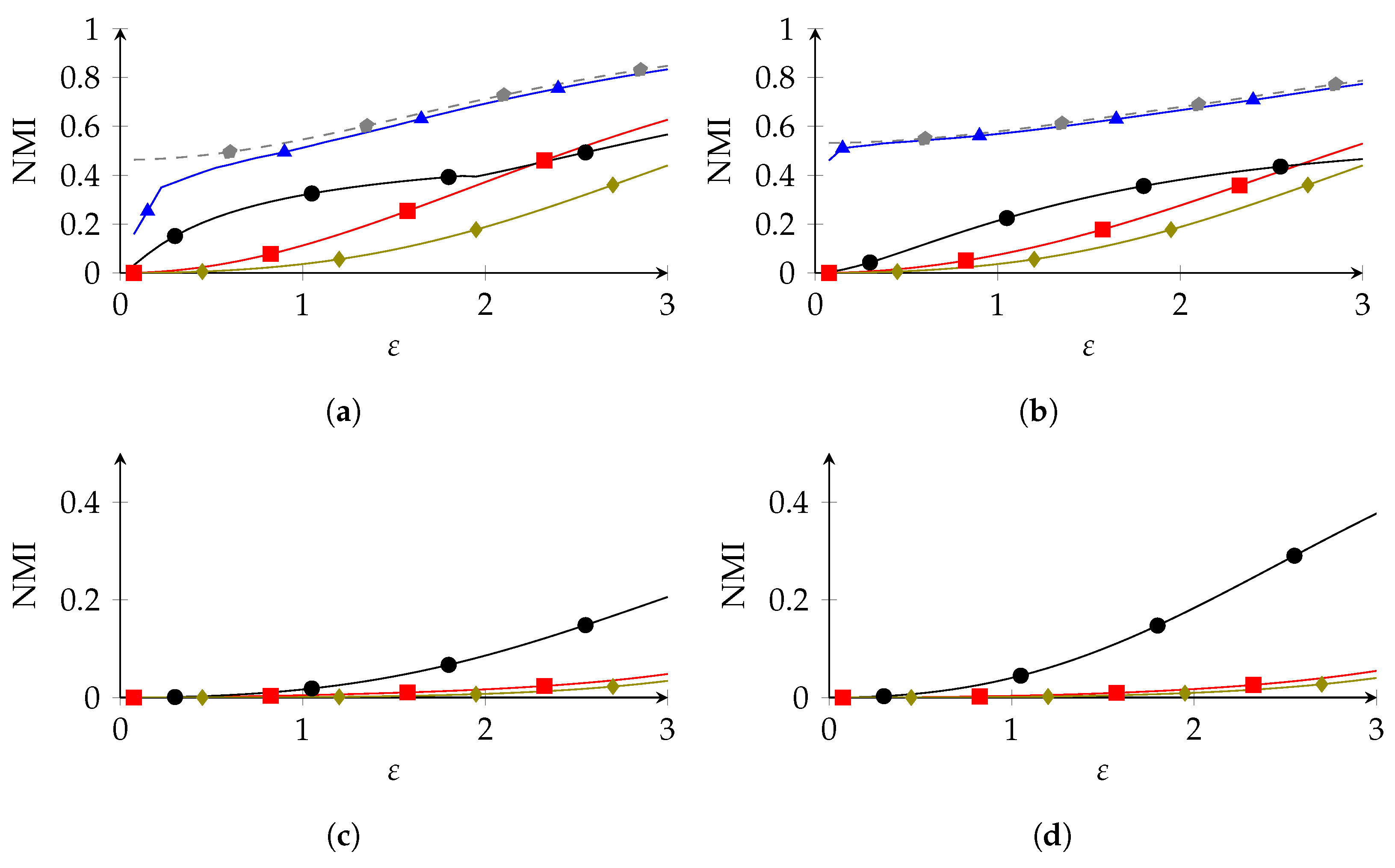
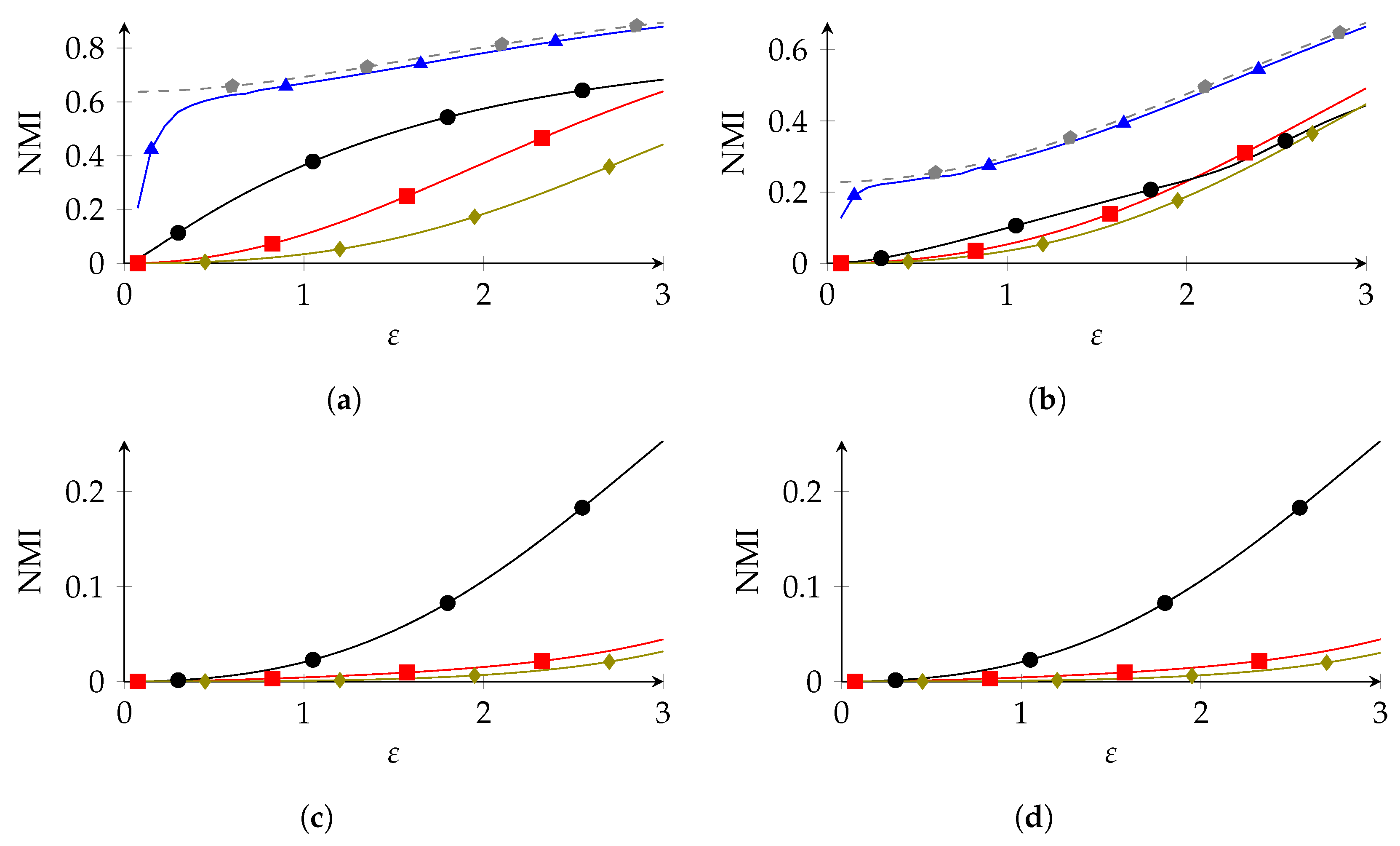
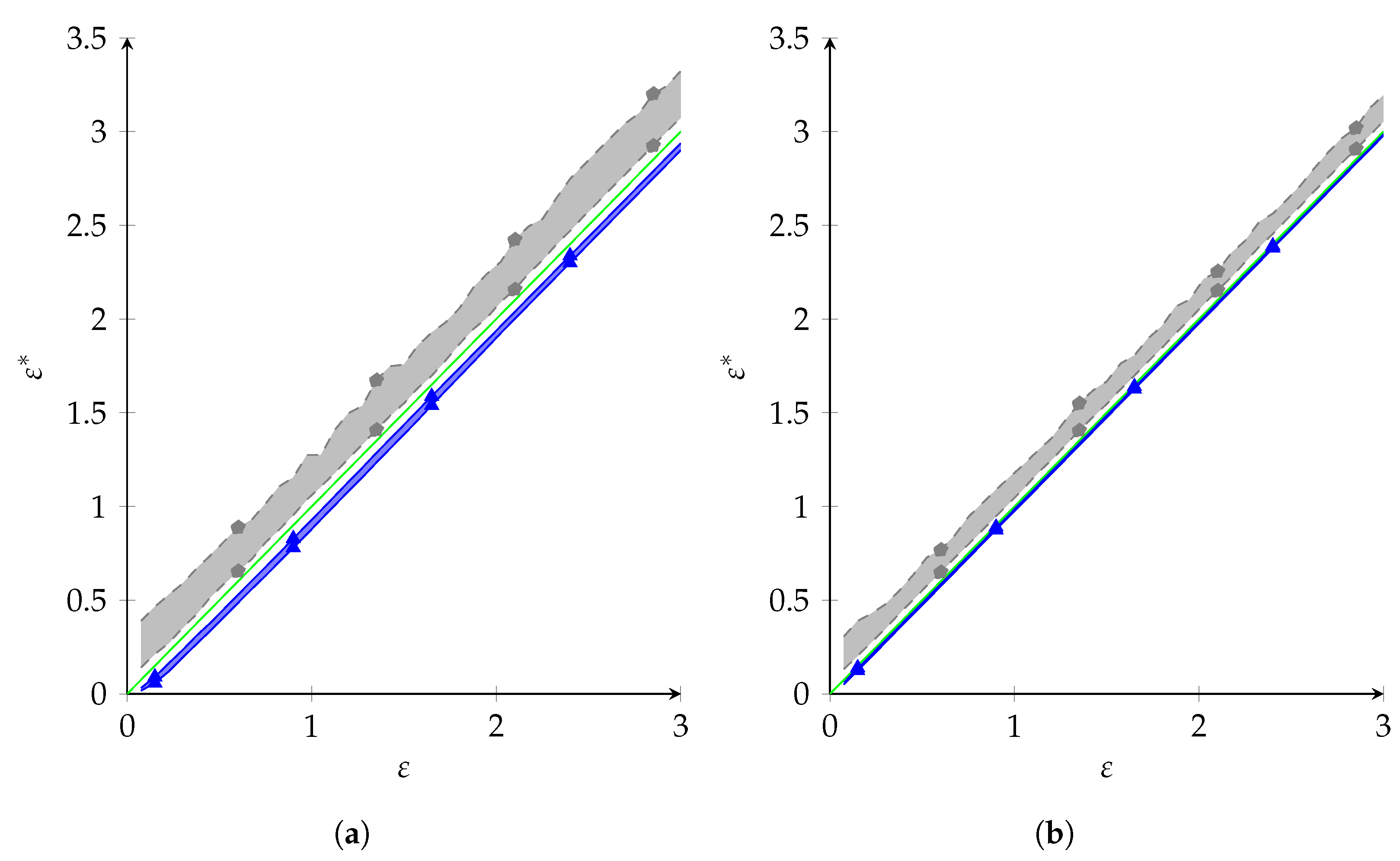
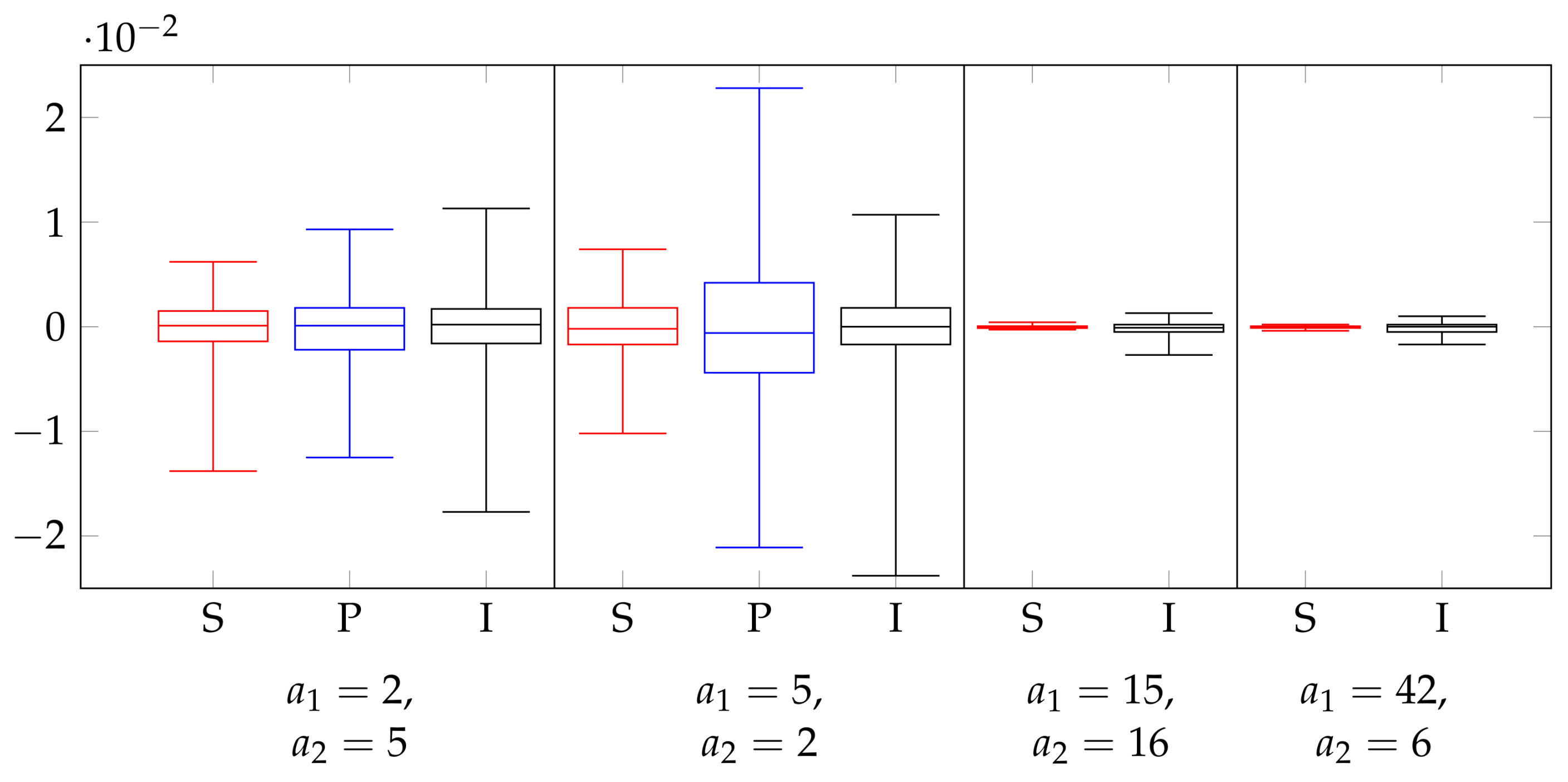
Table 1.
Notation used in this paper. ‘Page’ denotes the page the notation is first defined.
| Notation | Meaning | Page |
|---|---|---|
| sensitive data space | 6 | |
| non-sensitive data space | 6 | |
| 6 | ||
| 6 | ||
| user data | 6 | |
| ine | privacy mechanism | 6 |
| Q | matrix of | 6 |
| Y | 6 | |
| output space | 6 | |
| space of prob. dist. on | 6 | |
| true distribution | 6 | |
| estimated distribution | 7 | |
| I | mutual information | 8 |
| uncertainty set for P | 6 | |
| condition probability vector | 9 | |
| conditional projection of | 9 | |
| statistics of | 9 | |
| Rényi divergence | 10 | |
| PolyOpt | 13 | |
| Secret Randomized Response | 17 | |
| Independent Reporting | 18 |
Table 2.
NMI for synthetic data for various values of ().
| 0.1 | 0.01 | 0.001 | 0.1 | 0.01 | 0.001 | |
| SRR | 0.231 | 0.231 | 0.231 | 0.126 | 0.126 | 0.126 |
| PolyOpt | 0.727 | 0.723 | 0.719 | 0.374 | 0.372 | 0.370 |
| IR | 0.512 | 0.501 | 0.492 | 0.169 | 0.165 | 0.162 |
| 0.1 | 0.01 | 0.001 | 0.1 | 0.01 | 0.001 | |
| SRR | 0.009 | 0.009 | 0.009 | 0.005 | 0.005 | 0.005 |
| IR | 0.055 | 0.053 | 0.051 | 0.052 | 0.052 | 0.052 |
Disclaimer/Publisher’s Note: The statements, opinions and data contained in all publications are solely those of the individual author(s) and contributor(s) and not of MDPI and/or the editor(s). MDPI and/or the editor(s) disclaim responsibility for any injury to people or property resulting from any ideas, methods, instructions or products referred to in the content. |
© 2024 by the authors. Licensee MDPI, Basel, Switzerland. This article is an open access article distributed under the terms and conditions of the Creative Commons Attribution (CC BY) license (https://creativecommons.org/licenses/by/4.0/).
Share and Cite
MDPI and ACS Style
Lopuhaä-Zwakenberg, M.; Goseling, J. Mechanisms for Robust Local Differential Privacy. Entropy 2024, 26, 233. https://doi.org/10.3390/e26030233
AMA Style
Lopuhaä-Zwakenberg M, Goseling J. Mechanisms for Robust Local Differential Privacy. Entropy. 2024; 26(3):233. https://doi.org/10.3390/e26030233
Chicago/Turabian StyleLopuhaä-Zwakenberg, Milan, and Jasper Goseling. 2024. "Mechanisms for Robust Local Differential Privacy" Entropy 26, no. 3: 233. https://doi.org/10.3390/e26030233
Note that from the first issue of 2016, this journal uses article numbers instead of page numbers. See further details here.