1. Introduction
In 1972, Cover [
1] introduced the two-receiver discrete memoryless broadcast channel
to model a system of downlink communication in which
X is the sender and
are the receivers. In the same paper, he proposed a coding scheme which resulted in the superposition coding inner bound (SCIB). It turns out that the SCIB is indeed the capacity region for two-receiver broadcast channels in which the receivers are comparable in the following partial orders: degraded [
2], less noisy [
3], and more capable [
3]. However, for a general broadcast channel the single-letter capacity region remains open.
To characterize the capacity region of a broadcast channel, a standard approach is to show that one inner bound matches another outer bound. Currently, the best inner bound for general broadcast channels is Marton’s inner bound (MIB) [
4], while the UV outer bound (UVOB) [
5] was the best outer bound until recently, when a better one called J version outer bound was proposed in [
6].
The evaluation of inner and outer bounds is critical in the following aspects: (1) the evaluation of an inner bound usually results in an optimal input distribution which can help in the design of practical coding schemes; (2) the identification of the capacity region of a particular broadcast channel through the comparison of one inner bound and one outer bound relies on the evaluation of these two bounds; and (3) when claiming to establish a new bound, it is necessary to show that the new bound strictly improves on old ones through the evaluation of bounds on a particular channel.
Remark 1. This is the full version of conference papers accepted by ISIT 2022 and 2023 [7,8]. However, this evaluation is usually difficult due to its non-convexity [
9]. To alleviate this issue, there exist a number of generic optimization algorithms, such as interior point [
10], active set [
10], and sequential quadratic programming [
11]. However, efficient algorithms should use the domain knowledge of information theory as well; from this viewpoint, we consider the Blahut–Arimoto (BA) algorithm, which is specially customized for information theory.
The original BA algorithm was independently developed by Blahut [
12] and Arimoto [
13] to calculate the channel capacity
for a general point-to-point channel
. The algorithm transforms the original maximization problem into an alternating maximization problem:
where the updating formulae are explicit within each iteration.
There have been numerous extensions of the BA algorithm to various scenarios in information theory. For example, [
14] applied the BA algorithm to compute the sum rate of the multiple-access channel. Later, using the idea from the BA algorithm, the whole capacity region of the multiple-access channel was formulated in [
15] as a rank-one constrained problem and solved by relaxation methods. It is beyond the scope of this paper to list all of these references. Instead, we discuss those papers closely related to computing the bounds on capacity regions of broadcast channels.
In [
16], the authors considered the capacity region of a degraded broadcast channel
, where receiver
Z is a degraded version of
Y.
In this scenario, the capacity region of the rate pairs
is known, and can be achieved by the simplified version of superposition coding. The supporting hyperplanes can be characterized as
Using a similar idea to that of the BA algorithm, the authors designed an algorithm to alternatively maximize the objective function.
The method in [
16] is directly applicable to less noisy broadcast channels, as the characterization of the capacity region is the same as that of the degraded case. However, this equivalence no longer holds for the more capable case, as this time the value of the supporting hyperplane
is characterized as a max–min optimization problem (e.g., see Equation (
14)). As a mater of fact, the supporting hyperplanes of the above-mentioned bounds, that is, SCIB, MIB, and UVOB, are all of the max–min form. The main issue is that the minimization part is inside the maximization part, which prevents the application of the BA algorithm to the whole problem.
The algorithms for calculating inner bounds and outer bounds for general broadcast channels are very limited. The authors of [
17] considered MIB (see
Section 3.2) and designed a BA algorithm to compute the sum rate
of the simplified version, where the auxiliary random variable
. The objective function,
is convex in
, which means that the maximum input
X is a function of
. Noticing this, the authors performed optimization over all fixed mappings
. However, discarding
W can result in a strictly smaller sum rate [
18], making it is necessary to consider the complete version of MIB.
In this paper, we seek to design BA algorithms for general broadcast channels in order to compute the following inner and outer bounds: SCIB, MIB, and UVOB. The key difference here is that the optimization problems are max–min problems, rather than only containing a maximization part. In
Table 1, we provide an intuitive comparison of related references.
The notation we use is as follows.
p denotes a fixed (conditional) probability distribution such as
, while
q and
Q are used for (conditional) probabilities that are changeable. Calligraphic letters such as
are used to denote sets. The use of square brackets in the function
means that
f is specified by the variable
g;
denotes
; and unless otherwise specified, we use the natural logarithm. To make the mathematical expressions more concise, we use the following abbreviations of the Kullback–Leibler divergences:
The organization is as follows. First, in
Section 2 we introduce the necessary background on the BA algorithm and its extension in [
16]. Then, in
Section 3 we extend the BA algorithm to the evaluation of SCIB, MIB, and UVOB. Convergence analyses of these algorithms are presented in
Section 4. Finally, in
Section 5 we perform numerical experiments to validate the effectiveness and efficiency of our algorithms.
4. Convergence Analysis
Here, we aim to show that certain convergence results hold if lies in a proper convex set which contains the global maximizer . For this purpose, we first introduce the first-order characterization of a concave function.
Lemma 4 (Lemma 3 in [
22]).
Given a convex set , a differentiable function f is concave in if and only if, for all , Similar to [
22], we use the superlevel set to construct the convex set
. Let
be the superlevel set of the objective function
of SCIB:
For a fixed
k, it is possible for
to contain more than one connected set. For
, we denote the connected set that contains
q as
.
Similarly, for MIB and UVOB we define the corresponding (connected) superlevel sets: , , , . Note that k here should not be confused with the notation indicating the number of iterations in the algorithms.
4.1. Superposition Coding Inner Bound
According to Theorem 3, the expression of the objective function of SCIB depends on the value of . Without loss of generality, we can consider the objective function depicted in Equation (16). An equivalent condition for to be concave is provided in the following lemma.
Lemma 5. Given a convex set with a distribution , then as depicted in Equation (16) is concave in if and only if, for all , , we havewhere denotes . The following lemma shows that
lies in the same connected superlevel set as that of
. The proof (see
Appendix C) is similar to that for Lemma 4 in [
16].
Lemma 6. In Algorithm 2, if , then .
Fixing
and letting
be the maximizer, the following theorem states that the function values
converge. The proof (see
Appendix C) is similar to that of Theorem 2.
Theorem 5. If for some k and , and if is concave in , then the sequence generated by Algorithm 2 converges monotonically from below to .
The following corollary is implied by the proof of Theorem 5.
Corollary 1. If for some k and , and if is concave in , then The above analyses deal with
for a fixed
. When
changes to
, the estimation for the one-step change in the function value is presented in the following proposition (see proof in
Appendix C).
Proposition 2. Given , suppose that Algorithm 2 converges to the optimal variables and such that and . Letting be updated using Equation (22) and letting be the initial point for the next round, we have 4.2. Marton’s Inner Bound
Next, we present the convergence results of the BA algorithm for MIB. The proofs are omitted, as they are similar to those for SCIB.
Lemma 7. Given a convex set with a distribution , as depicted in Equation (24) is concave in if and only if, for all , , we havewhere denotes . Lemma 8. In Algorithm 3, if , then .
Fixing and letting be the maximizer, the following theorem states that the function values converge.
Theorem 6. If for some k and and if is concave in , then the sequence generated by Algorithm 3 converges monotonically from below to .
The following corollary is implied by the proof of Theorem 6.
Corollary 2. If for some k and , and if is concave in , then The estimation for the one-step change in the function value for MIB is presented in the following proposition.
Proposition 3. Given , suppose that Algorithm 3 converges to the optimal variables and such that and . Letting be updated using Equation (27) and letting be the initial point for the next round, we have 4.3. UV Outer Bound
Now, we present the convergence results of of the BA algorithm for UVOB. The proofs are again omitted, as they are similar to those of SCIB.
Lemma 9. Given a convex set of distribution , as depicted in Equation (29) is concave in if and only if, for all , , we havewhere denotes . Lemma 10. In Algorithm 4, if , then .
Fixing and letting be the maximizer, the following theorem states that the function values converge.
Theorem 7. If for some k and , and if is concave in , then the sequence generated by Algorithm 4 converges monotonically from below to .
The following corollary is implied by the proof of Theorem 7.
Corollary 3. If for some k and , and if is concave in , then The estimation for the one-step change in the function value for UVOB is presented in the following proposition.
Proposition 4. Given , suppose that Algorithm 4 converges to the optimal variables and such that and . Letting be updated using Equations (39) and (40) and letting be the initial point for the next round, we have 5. Numerical Results
We take the binary skew-symmetric broadcast channel
as the test channel. The conditional probability matrices are
This is perhaps the simplest broadcast channel for which the capacity region is still unknown.
This broadcast channel plays a very important role in research on capacity bounds. It was first studied in [
23] to show that the time-sharing random variable is useful for the Cover–van der Meulen inner bound [
24,
25]. Later, [
26,
27,
28] demonstrated that the sum rate of the UVOB for this broadcast channel is strictly larger than that of the MIB, showing for the first time that at least one of these two bounds are suboptimal.
Our algorithms are important in at least the following sense: supposing that it is not known whether the MIB matches the UVOB (or the other two bounds for a new scenario) and we want to check this; we can perform an exhaustive search on channel matrices of size
(or of higher dimensions) to check whether they match. According to the results shown below in
Section 5.5, this does not take very much time compared with generic algorithms.
In the following, we apply the algorithms to compute the value of the supporting hyperplane , where . The initial values of and are . This set of parameters is feasible for UVOB, as .
We demonstrate the algorithms in the following aspects: (1) the maximization part; (2) the minimization part; (3) the change from the maximum part to the minimization part; (4) the superlevel set; and (5) comparison with generic non-convex algorithms.
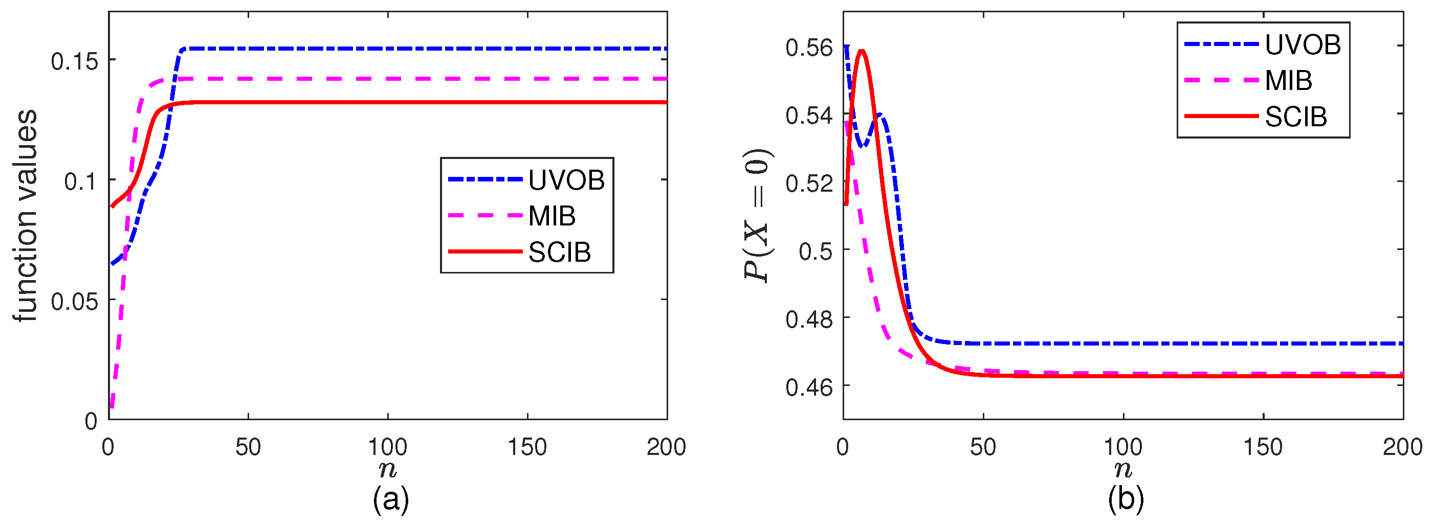
5.1. Maximization Part
In this part, we fix
and
to the initial values and let the BA algorithms iterate for
times. The results are presented in
Figure 1. Because this is the maximization part, the function values increase as the iterations proceed. It is clear that the function values behave properly for fixed
and
.
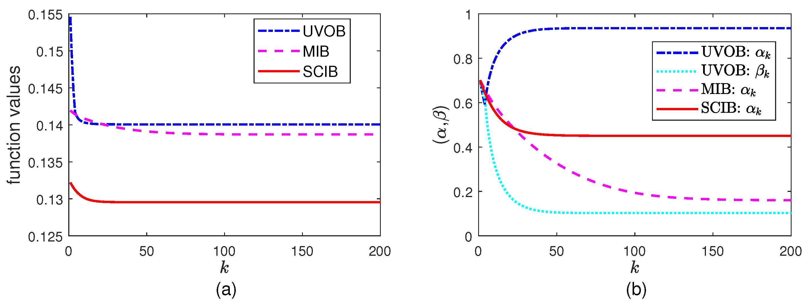
5.2. Minimization Part
In this part, we start with the initial
and
, then let the algorithms iterate for
times. The results for
are presented in
Figure 2. Because this is the minimization part, the function values decrease as the iterations proceed. It is clear that
in SCIB and MIB gradually changes as
k grows. For UVOB, it is necessary to ensure that
. When the updated
makes
fall below this value, it becomes necessary to scale it back. This happens approximately starting from
.
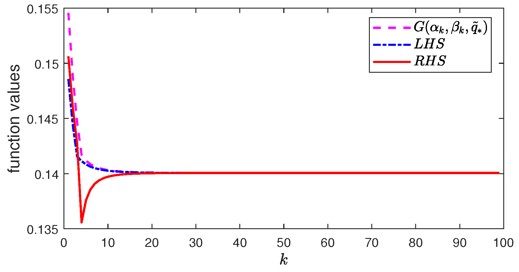
5.3. Change from Maximization to Minimization
In this part, we consider UVOB and let
K in the algorithm be
.
Figure 3 plots the following three values in Equation (
43):
As the algorithm iterates, the estimate in Equation (
43) becomes more and more accurate, as
and
for small
x.
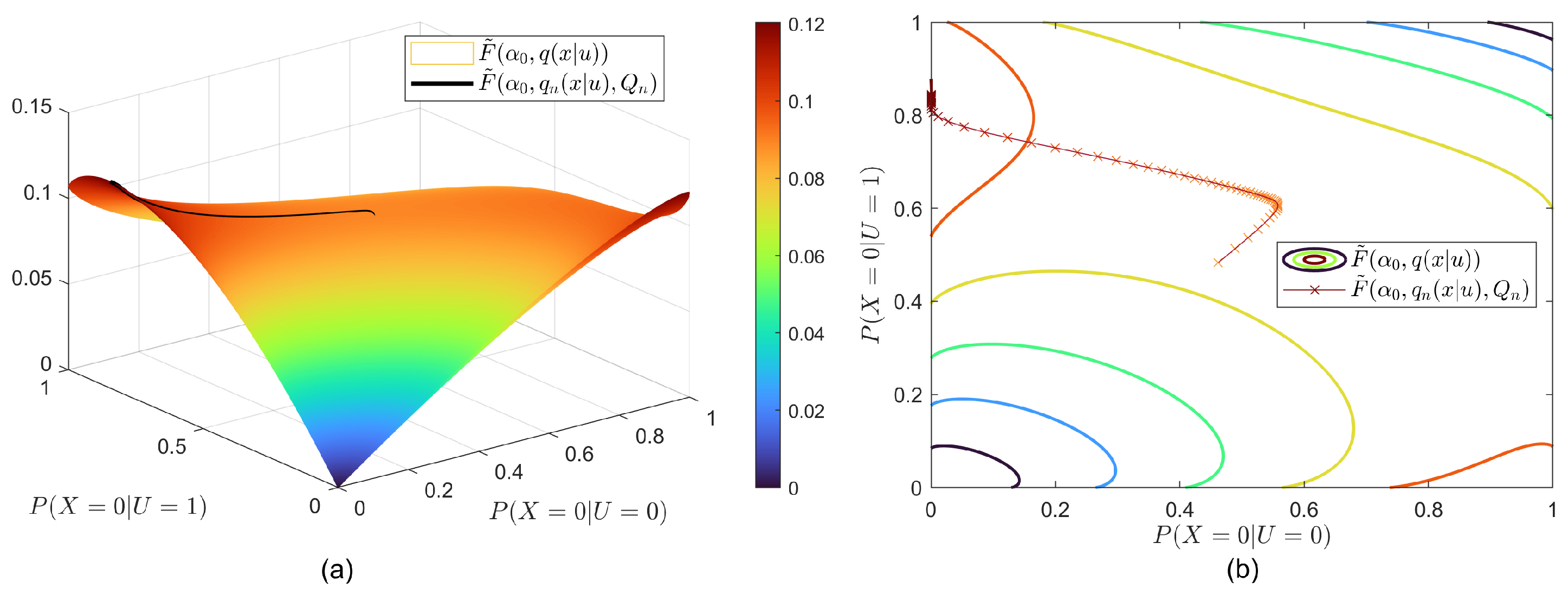
5.4. Superlevel Set
To visualize the convergence of
and its relation with the superlevel set, we take SCIB as an example and fix
such that
has two free variables. We reformulate the objective function of SCIB depicted in Equation (16) as follows:
where
In particular, we fix
and
, then use the algorithm to find the values of
and
. The results are shown in
Figure 4. In this case,
for large enough
n lies in the concave part of the superlevel set, meaning that the algorithm converges. Here, it should be mentioned that it is possible that the algorithm may not converge to the optimal point for some initial
s that do not lie in the concave part.
5.5. Comparison with Generic Non-Convex Algorithms
Here, we compare our algorithms with the following generic algorithms implemented using the “fmincon” MATLAB function: interior-point, active-set, and sequential quadratic programming (sqp). For simplicity, we only compare the sum rate of MIB, for which the optimal value is 0.2506717… nats (0.3616428… bits). The optimization problem for computing the sum rate is
According to Lemma 3, the cardinality size is
.
Notice that we do not carry out a comparison with the method in [
16], as it cannot be applied to cases where there is a minimum. For scenarios in which [
16] can be used, our algorithms degenerate to the method in [
16].
The initial point of
is randomly generated for all the algorithms.
Table 2 lists the experimental results. For the first three algorithms, a randomly picked starting point usually does not provide a good enough result. Thus, we ran the first three algorithms multiple times until the best function value hit 0.2506 in order to test their effectiveness. It is clear from the table that only sqp can be considered comparable to our algorithms.
For further comparison with sqp, we randomly generated broadcast channels with cardinalities of
, 4, 5, 6, and
. The corresponding dimensions are
, 512, 1125, 2160. Because the optimal sum rate is not yet known, we ran sqp once to record the running time. The results in
Table 3 suggest that our algorithms are highly scalable. This meets our expectation, as the updating formulae in Equations (
5) and (
7) are all explicit and can be computed rapidly.


