
Analysis of Vibration Signals Based on Machine Learning for Crack Detection in a Low-Power Wind Turbine
 , , and
Abstract
:1. Introduction
2. Theoretical Background
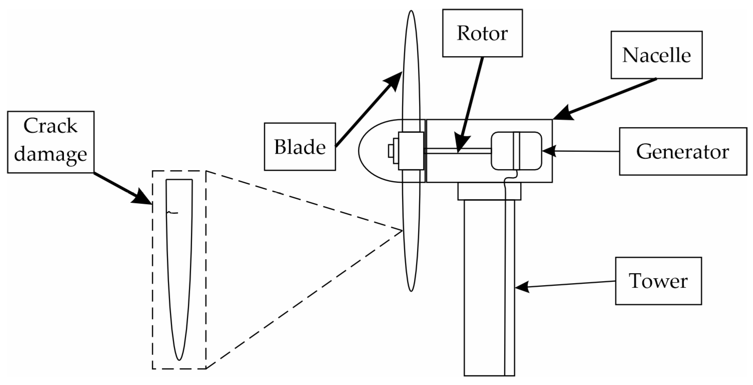
2.1. Wind Turbine
Vibration Model
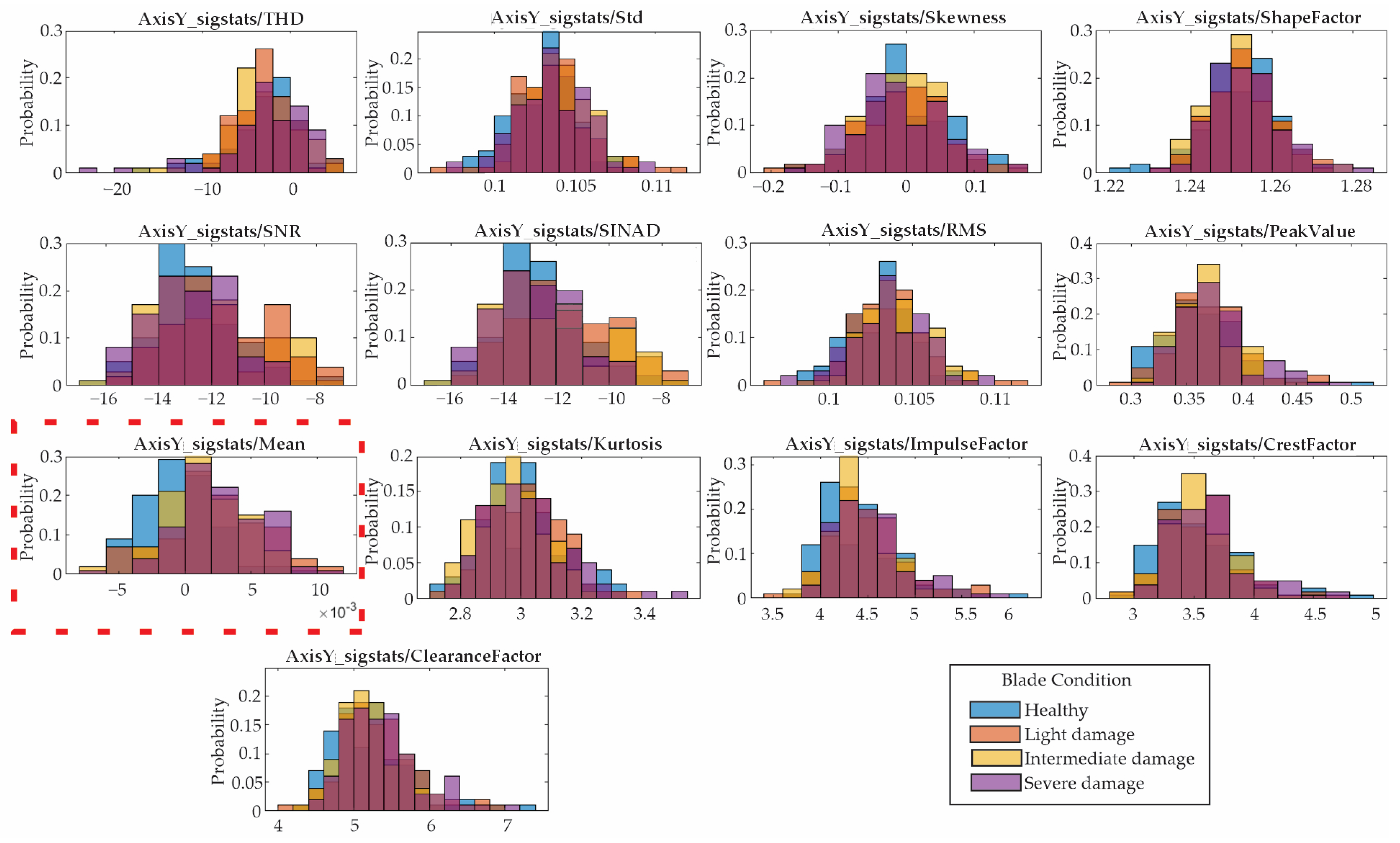
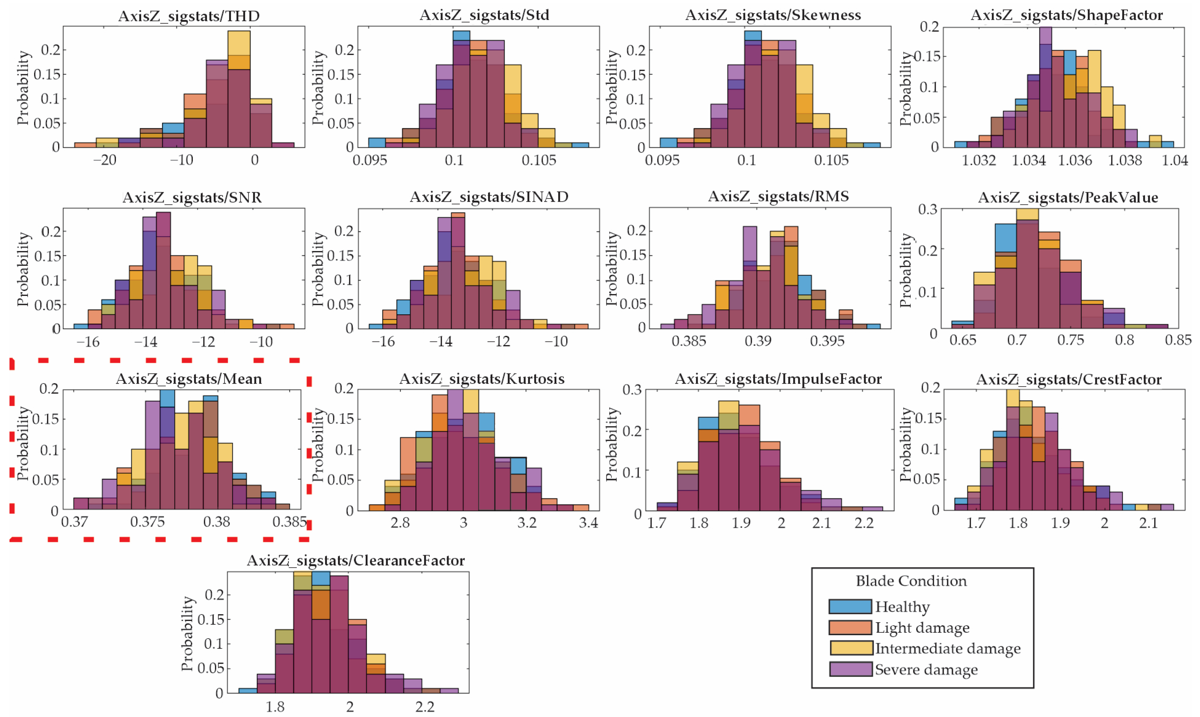
2.2. Signal Features
2.2.1. Statistical Features
2.2.2. Impulsive Metrics
2.2.3. Signal Processing Metrics
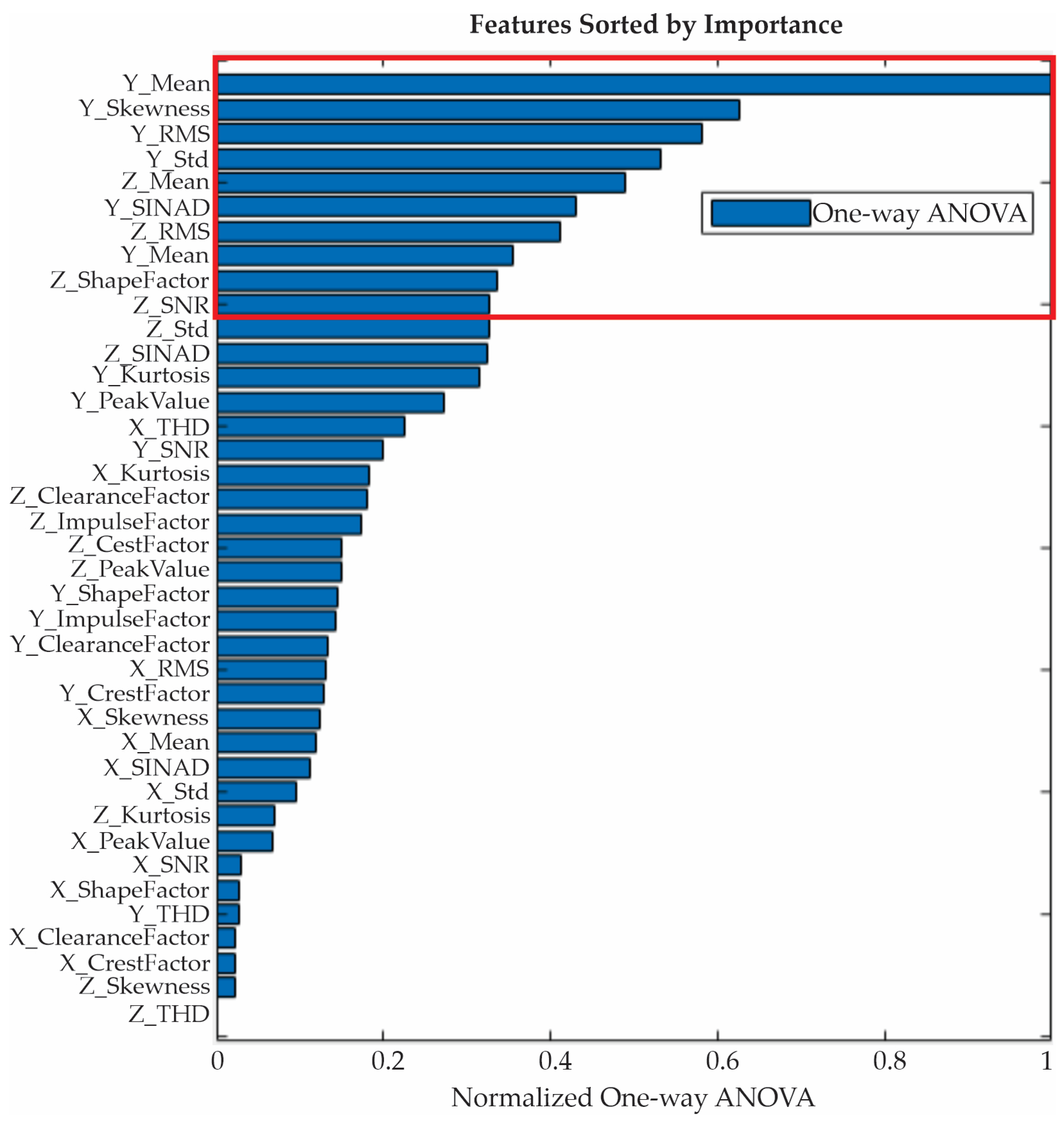
2.3. One-Way Analysis of Variance (ANOVA)
2.4. Machine Learning Classifiers
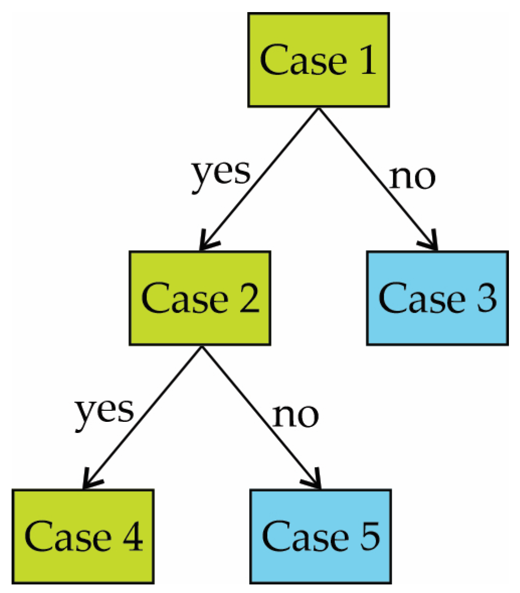
2.4.1. Decision Tree
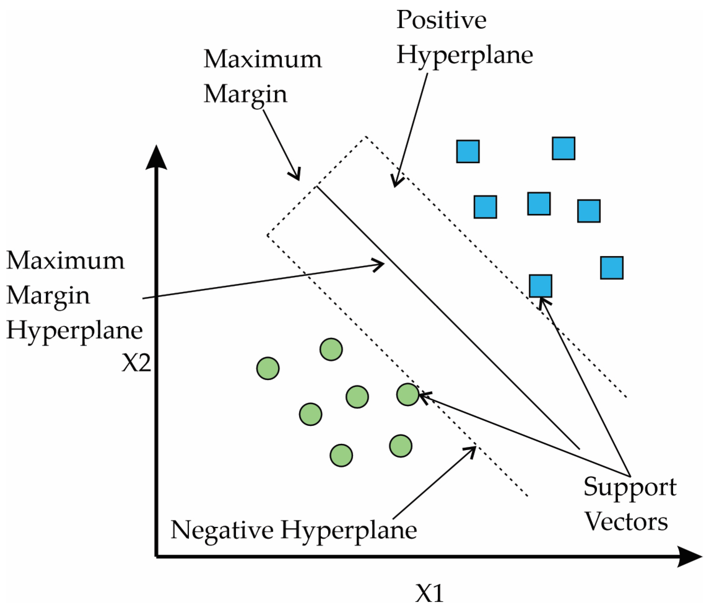
2.4.2. Support Vector Machine
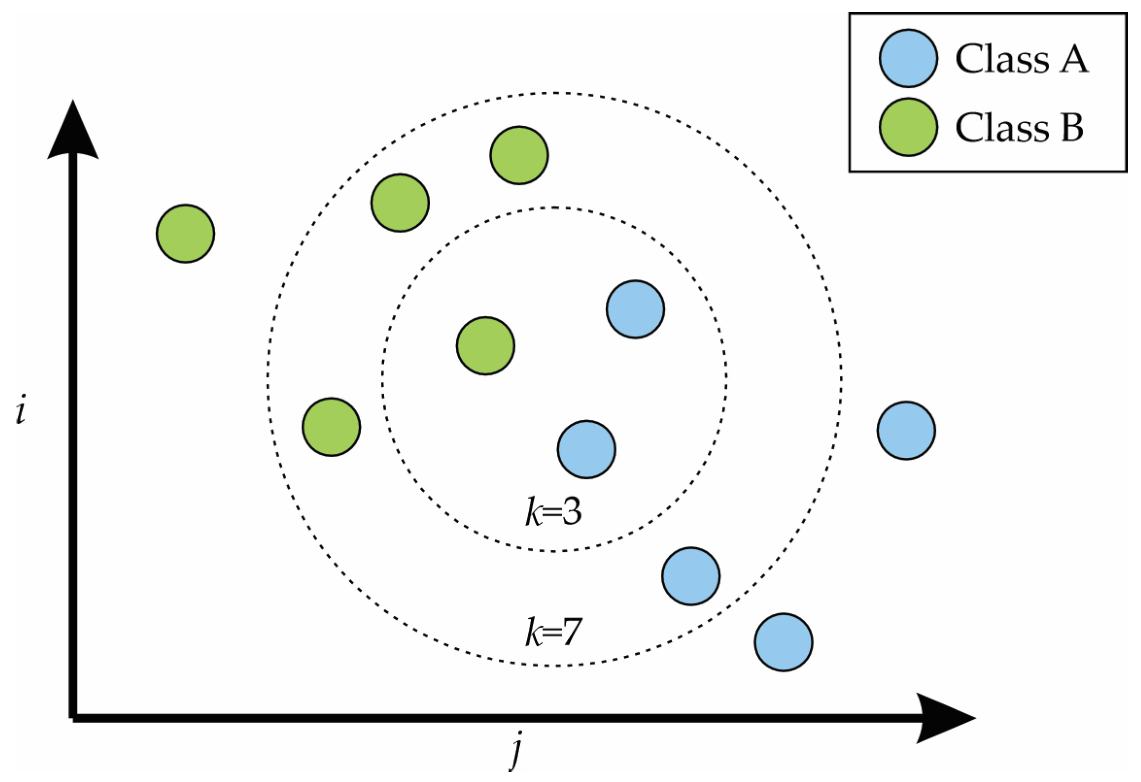
2.4.3. K-Nearest Neighbors
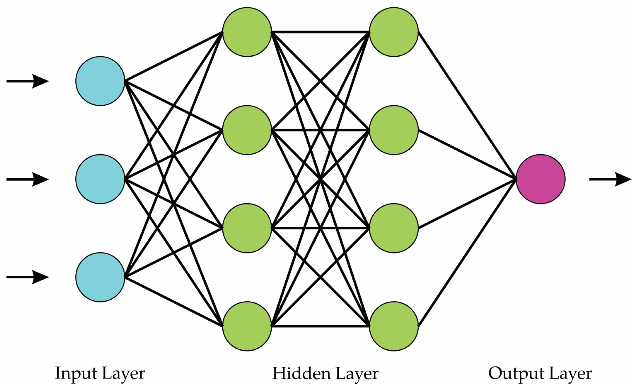
2.4.4. Neural Network
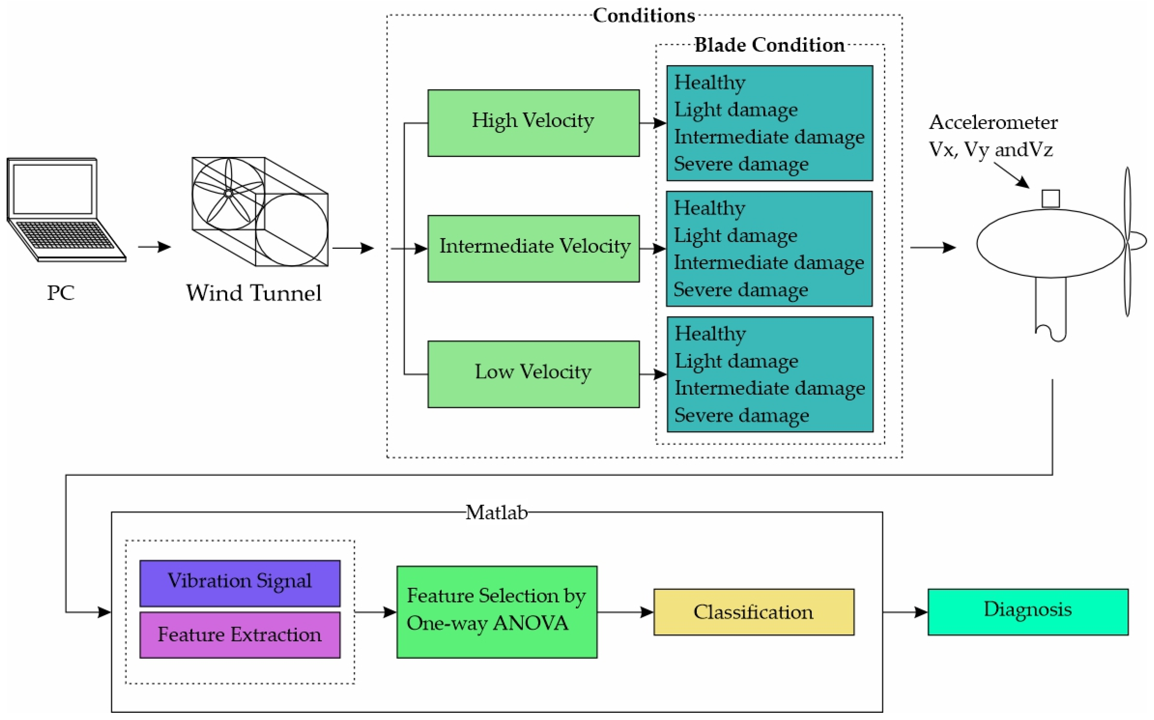
3. Methodology
4. Experimental Setup and Results
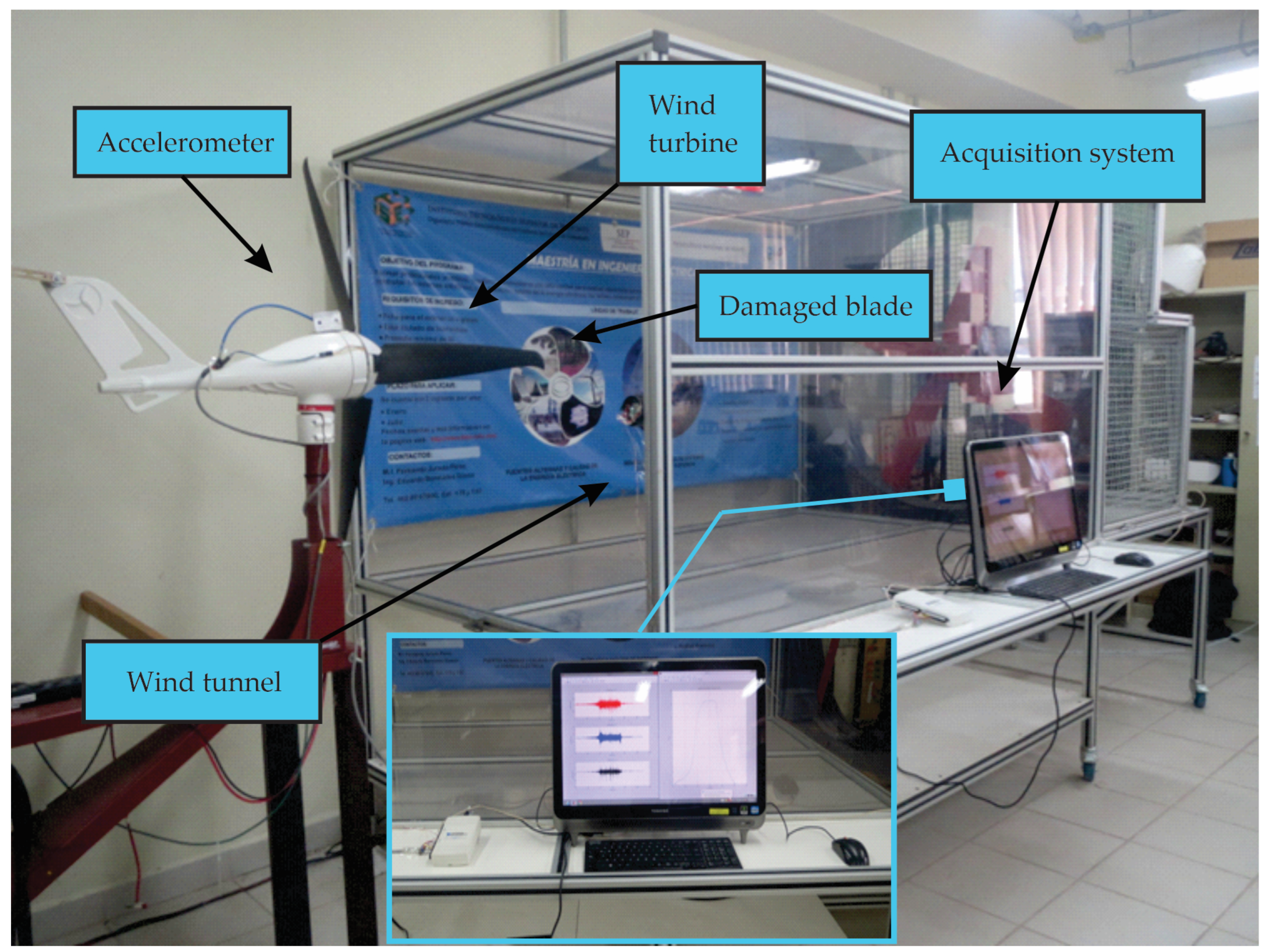
4.1. Experimental Setup
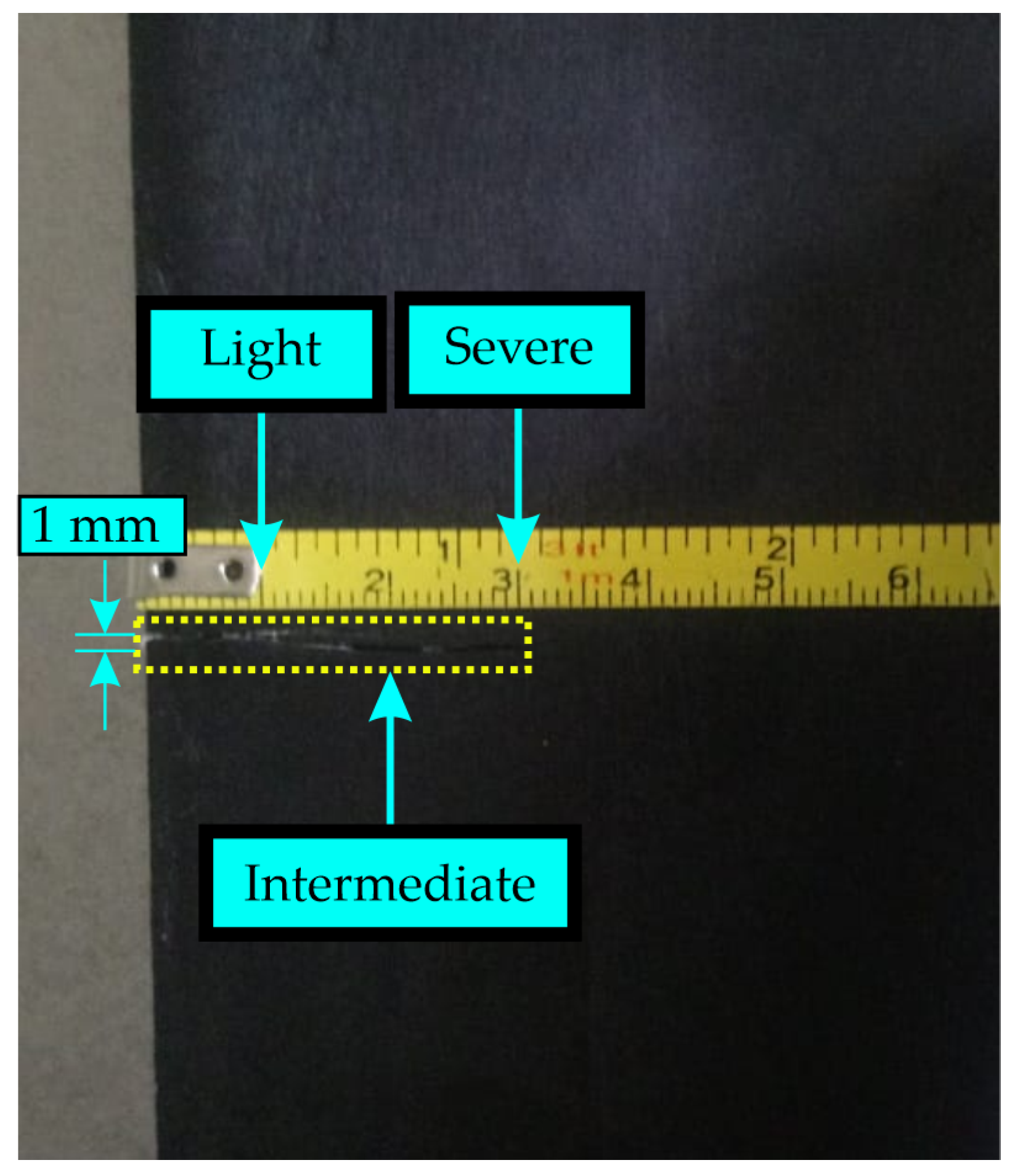
4.2. Crack Information
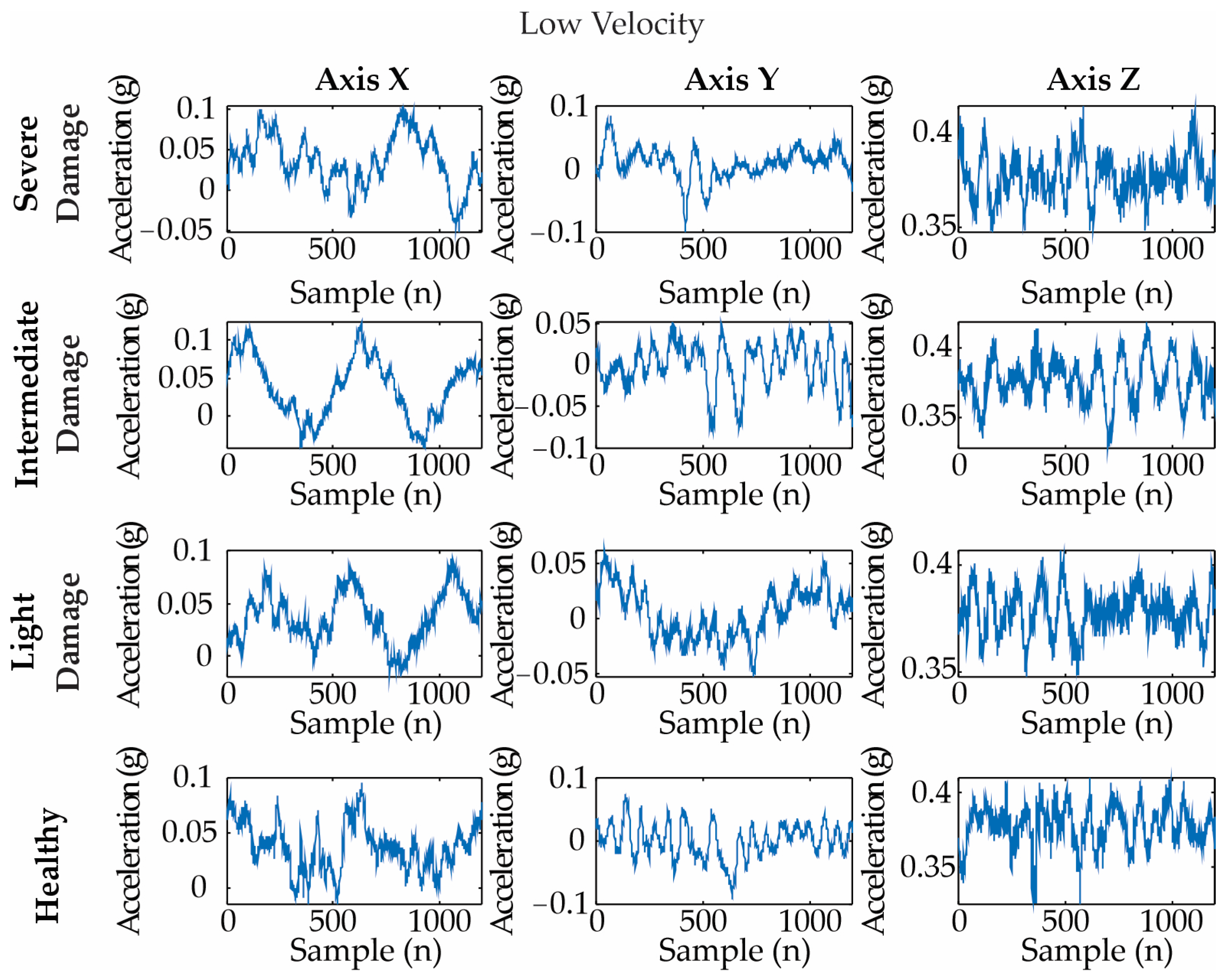
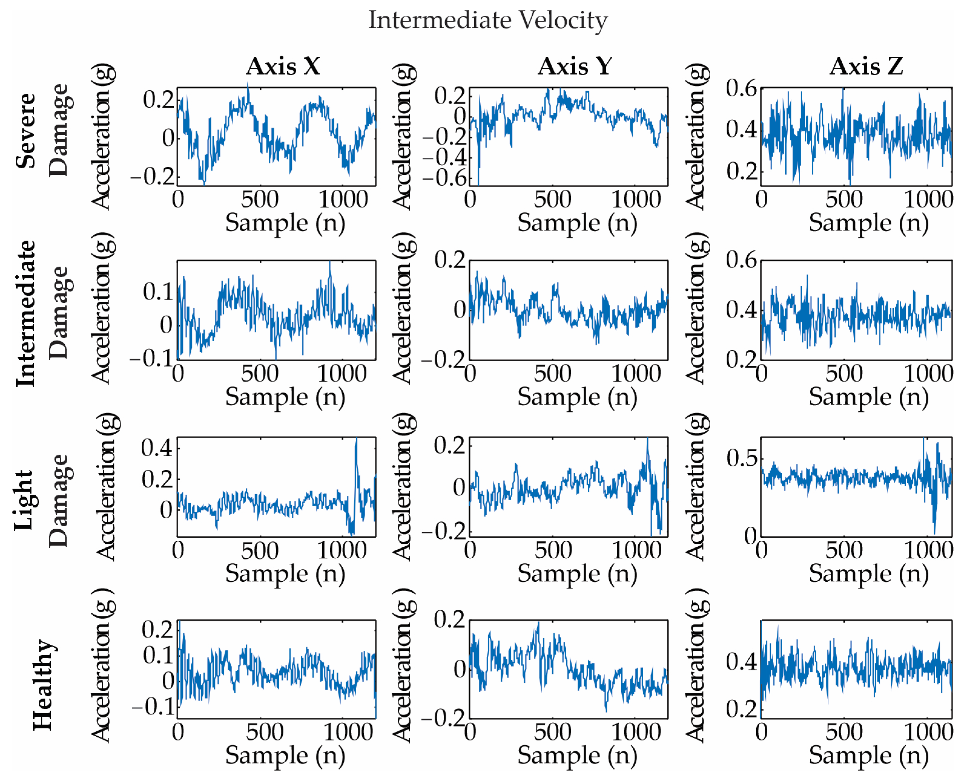
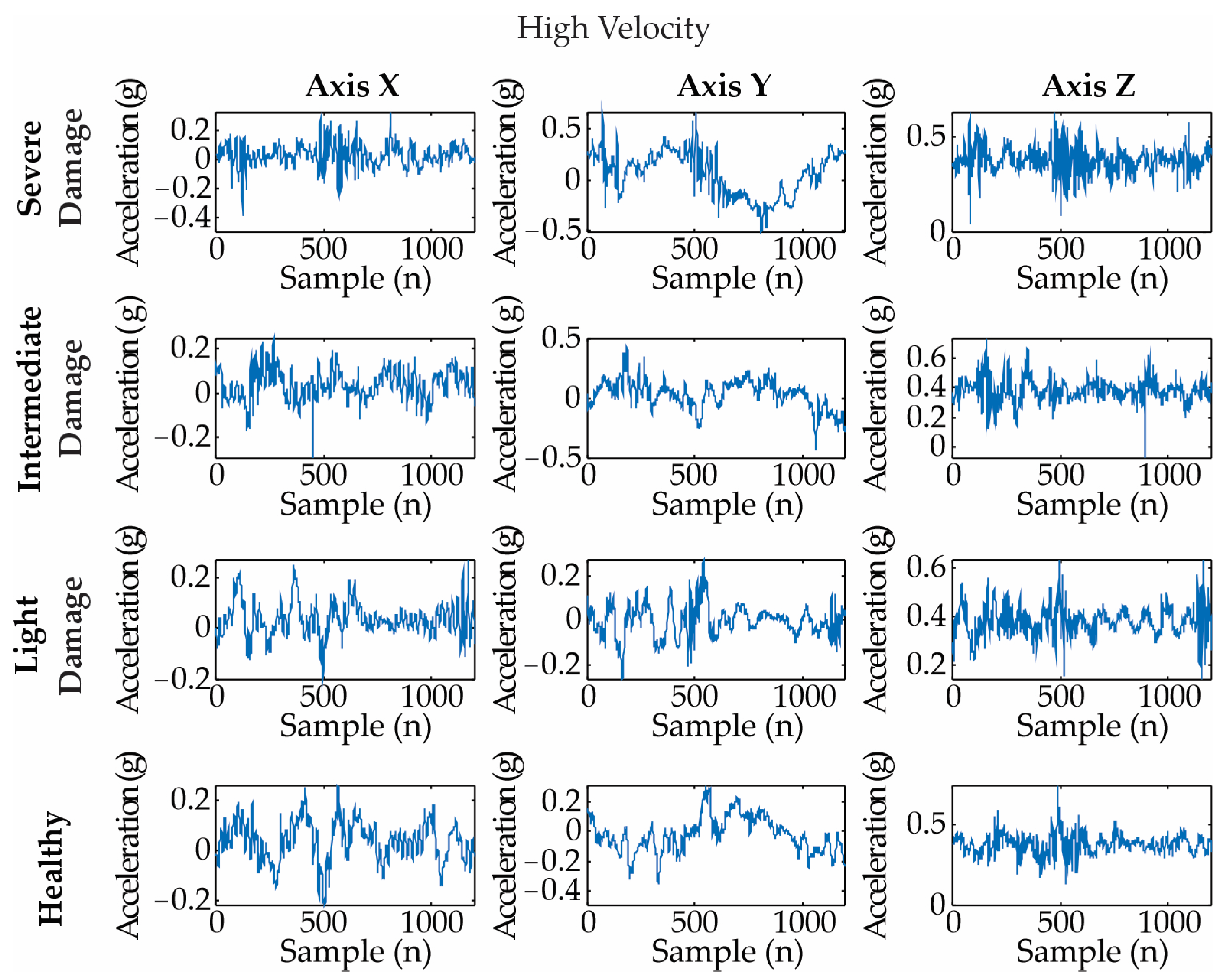
4.3. Vibration Signals
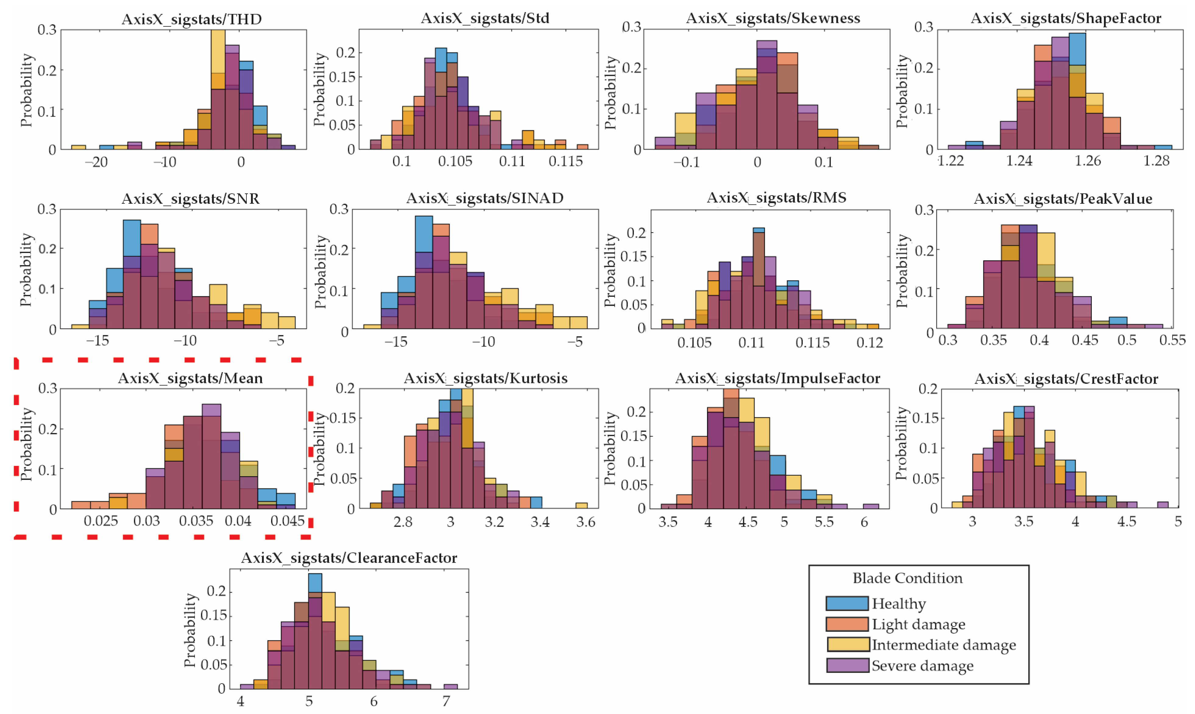
4.4. Statistical Feature Selection
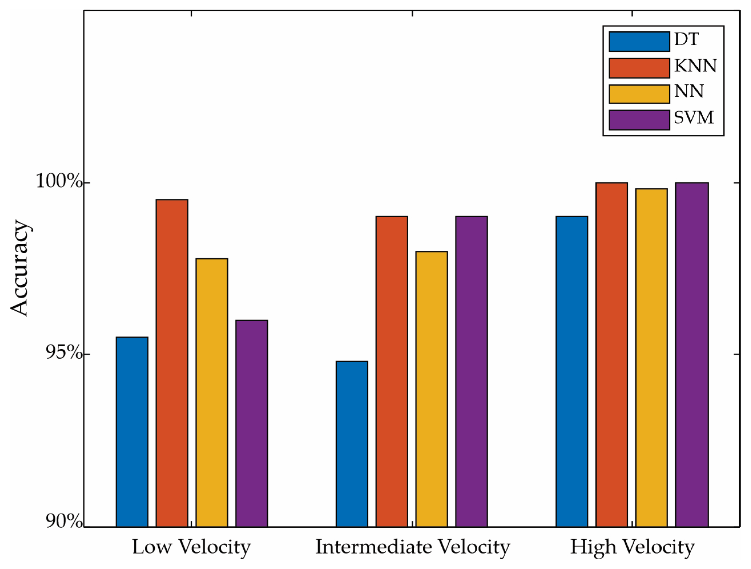
4.5. Classifiers
5. Conclusions
Author Contributions
Funding
Institutional Review Board Statement
Informed Consent Statement
Data Availability Statement
Acknowledgments
Conflicts of Interest
Abbreviations
| ANOVA | Analysis of Variance |
| DT | Decision Tree |
| EEMD | Ensemble Empirical Mode Decomposition |
| FFT | Fast Fourier Transform |
| FPGA | Field programmable gate array |
| KNN | K-Nearest Neighbor |
| ML | Machine learning |
| NN | Neural Network |
| RMS | Root Mean Square |
| RSSA | Recursive singular spectrum analysis |
| SINAD | Signal-to-Noise and Distortion ratio |
| SNR | Signal-to-noise Ratio |
| SVM | Support Vector Machine |
| THD | Total Harmonic Distortion |
| WT | Wind turbine |
References
- Global Wind Energy Council. Global Wind Report 2021; Global Wind Energy Council: Brussels, Belgium, 2021; pp. 6–7. [Google Scholar]
- Markiewicz, M.; Pająk, M.; Muślewski, Ł. Analysis of Exhaust Gas Content for Selected Biofuel-Powered Combustion Engines with Simultaneous Modification of Their Controllers. Materials 2021, 14, 7621. [Google Scholar] [CrossRef]
- Kaewniam, P.; Cao, M.; Alkayem, N.F.; Li, D.; Manoach, E. Recent advances in damage detection of wind turbine blades: A state-of-the-art review. Renew. Sustain. Energy Rev. 2022, 167, 112723. [Google Scholar] [CrossRef]
- Rangel-Rodriguez, A.-H.; Huerta-Rosales, J.R.; Amezquita-Sanchez, J.P.; Granados-Lieberman, D.; Bueno-Lopez, M.; Valtierra-Rodriguez, M. Detection of Multiple Faults in a Low-Power Wind Turbine by using Convolutional Neural Networks. In Proceedings of the 2022 IEEE International Autumn Meeting on Power, Electronics and Computing (ROPEC), Ixtapa, Mexico, 9–11 November 2022; pp. 1–6. [Google Scholar]
- Zhang, C.; Chen, H.P.; Huang, T.L. Fatigue damage assessment of wind turbine composite blades using corrected blade element momentum theory. Measurement 2018, 129, 102–111. [Google Scholar] [CrossRef]
- Li, D.; Ho, S.-C.M.; Song, G.; Ren, L.; Li, H. A review of damage detection methods for wind turbine blades. Smart Mater. Struct. 2015, 24, 033001. [Google Scholar] [CrossRef]
- Ciang, C.C.; Lee, J.R.; Bang, H.J. Structural health monitoring for a wind turbine system: A review of damage detection methods. Meas. Sci. Technol. 2008, 19, 122001. [Google Scholar] [CrossRef] [Green Version]
- Bo, Z.; Yanan, Z.; Changzheng, C. Acoustic emission detection of fatigue cracks in wind turbine blades based on blind deconvolution separation. Fatigue Fract. Eng. Mater. Struct. 2016, 40, 959–970. [Google Scholar] [CrossRef]
- Awadallah, M.; El-Sinawi, A. Effect and detection of cracks on small wind turbine blade vibration using special Kriging analysis of spectral shifts. Measurement 2020, 151, 107076. [Google Scholar] [CrossRef]
- Liu, Y.; Hajj, M.; Bao, Y. Review of robot-based damage assessment for offshore wind turbines. Renew. Sustain. Energy Rev. 2022, 158, 112187. [Google Scholar] [CrossRef]
- Xia, J.; Zou, G. Operation and maintenance optimization of offshore wind farms based on digital twin: A review. Ocean Eng. 2023, 268, 113322. [Google Scholar] [CrossRef]
- Yang, W.; Peng, Z.; Wei, K.; Tian, W. Structural health monitoring of composite wind turbine blades: Challenges, issues and potential solutions. IET Renew. Power Gener. 2017, 11, 411–416. [Google Scholar] [CrossRef] [Green Version]
- Grasse, F.; Trappe, V.; Thöns, S.; Said, S. Structural health monitoring of wind turbine blades by strain measurement and vibration analysis. In Proceedings of the EURODYN 2011—8th International conference on structural dynamics, Leuven, Belgium, 4–6 July 2011. [Google Scholar]
- Pacheco-Chérrez, J.; Probst, O. Vibration-based damage detection in a wind turbine blade through operational modal analysis under wind excitation. Mater. Today: Proc. 2022, 56, 291–297. [Google Scholar] [CrossRef]
- Teng, W.; Ding, X.; Tang, S.; Xu, J.; Shi, B.; Liu, Y. Vibration Analysis for Fault Detection of Wind Turbine Drivetrains—A Comprehensive Investigation. Sensors 2021, 21, 1686. [Google Scholar] [CrossRef]
- Pająk, M.; Muślewski, Ł.; Kluczyk, M.; Kolar, D.; Landowski, B.; Kałaczyński, T. Identification of Reliability States of a Ship Engine of the Type Sulzer 6AL20/24. SAE Int. J. Engines 2021, 15, 527–542. [Google Scholar] [CrossRef]
- Ha, J.M.; Oh, H.; Park, J.; Youn, B.D. Classification of operating conditions of wind turbines for a class-wise condition monitoring strategy. Renew. Energy 2017, 103, 594–605. [Google Scholar] [CrossRef]
- Colone, L.; Hovgaard, M.; Glavind, L.; Brincker, R. Mass detection, localization and estimation for wind turbine blades based on statistical pattern recognition. Mech. Syst. Signal Process. 2018, 107, 266–277. [Google Scholar] [CrossRef]
- Wang, W.; Yang, J.; Dai, J.; Chen, A. EEMD-based videogrammetry and vibration analysis method for rotating wind power blades. Measurement 2023, 207, 112423. [Google Scholar] [CrossRef]
- Stetco, A.; Dinmohammadi, F.; Zhao, X.; Robu, V.; Flynn, D.; Barnes, M.; Keane, J.; Nenadic, G. Machine learning methods for wind turbine condition monitoring: A review. Renew. Energy 2019, 133, 620–635. [Google Scholar] [CrossRef]
- Wang, L.; Zhang, Z. Automatic Detection of Wind Turbine Blade Surface Cracks Based on UAV-Taken Images. IEEE Trans. Ind. Electron. 2017, 64, 7293–7303. [Google Scholar] [CrossRef]
- Joshuva, A.; Sugumaran, V. A data driven approach for condition monitoring of wind turbine blade using vibration signals through best-first tree algorithm and functional trees algorithm: A comparative study. ISA Trans. 2017, 67, 160–172. [Google Scholar] [CrossRef] [PubMed]
- Shihavuddin, A.; Chen, X.; Fedorov, V.; Christensen, A.N.; Riis, N.A.B.; Branner, K.; Dahl, A.B.; Paulsen, R.R. Wind Turbine Surface Damage Detection by Deep Learning Aided Drone Inspection Analysis. Energies 2019, 12, 676. [Google Scholar] [CrossRef] [Green Version]
- Tang, Y.; Chang, Y.; Li, K. Applications of K-nearest neighbor algorithm in intelligent diagnosis of wind turbine blades damage. Renew. Energy 2023, 212, 855–864. [Google Scholar] [CrossRef]
- Mucchielli, P.; Bhowmik, B.; Ghosh, B.; Pakrashi, V. Real-time accurate detection of wind turbine downtime-an Irish perspective. Renew. Energy 2021, 179, 1969–1989. [Google Scholar] [CrossRef]
- Bhowmik, B.; Tripura, T.; Hazra, B.; Pakrashi, V. First-order eigen-perturbation techniques for real-time damage detection of vibrating systems: Theory and applications. Appl. Mech. Rev. 2019, 76, 060801. [Google Scholar] [CrossRef]
- Bhowmik, B.; Hazra, B.; Pakrashi, V. Real-Time Structural Health Monitoring of Vibrating Systems; CRC Press: Boca Raton, FL, USA, 2022. [Google Scholar]
- Bhowmik, B.; Krishnan, M.; Hazra, B.; Pakrashi, V. Real-time unified single-and multi-channel structural damage detection using recursive singular spectrum analysis. Struct. Health Monit. 2019, 18, 563–589. [Google Scholar] [CrossRef]
- Bhowmik, B.; Panda, S.; Hazra, B.; Pakrashi, V. Feedback-driven error-corrected single-sensor analytics for real-time condition monitoring. Int. J. Mech. Sci. 2022, 214, 106898. [Google Scholar] [CrossRef]
- Xu, D.; Liu, P.; Chen, Z.; Leng, J.; Jiao, L. Achieving robust damage mode identification of adhesive composite joints for wind turbine blade using acoustic emission and machine learning. Compos. Struct. 2019, 236, 111840. [Google Scholar] [CrossRef]
- Joshuva, A.; Sugumaran, V. A lazy learning approach for condition monitoring of wind turbine blade using vibration signals and histogram features. Measurement 2019, 152, 107295. [Google Scholar] [CrossRef]
- Kamran, M. Chapter 6—Planning and modeling of wind energy systems. In Fundamentals of Smart Grid Systems; Academic Press: Cambridge, MA, USA, 2023; pp. 271–298. [Google Scholar]
- Xu, J.; Ding, X.; Gong, Y.; Wu, N.; Yan, H. Rotor imbalance detection and quantification in wind turbines via vibration analysis. Wind. Eng. 2021, 46, 3–11. [Google Scholar] [CrossRef]
- The MathWorks, Inc. Signal Features. Available online: https://la.mathworks.com/help/predmaint/ug/signal-features.html (accessed on 29 March 2023).
- The MathWorks, Inc. One-Way ANOVA. Available online: https://la.mathworks.com/help/stats/one-way-anova.html (accessed on 12 April 2023).
- Loh, W.-Y. Fifty Years of Classification and Regression Trees. Int. Stat. Rev. 2014, 82, 329–348. [Google Scholar] [CrossRef] [Green Version]
- Castañeda, R.A.M. Implementación del método máquinas de soporte vectorial en bases de datos espaciales para análisis de clasificación supervisada en imágenes de sensores remotos. Rev. Cart. 2021, 102, 27–42. [Google Scholar]
- Huerta-Rosales, J.R.; Granados-Lieberman, D.; Garcia-Perez, A.; Camarena-Martinez, D.; Amezquita-Sanchez, J.P.; Valtierra-Rodriguez, M. Short-Circuited Turn Fault Diagnosis in Transformers by Using Vibration Signals, Statistical Time Features, and Support Vector Machines on FPGA. Sensors 2021, 21, 3598. [Google Scholar] [CrossRef] [PubMed]
- Dimitrios, K.; Dimitrios, M.; Xanthoula-Eirini, P.; Gravalos, I.; Sawalhi, N.; Loutridis, S. A machine learning approach for the condition monitoring of rotating machinery. J. Mech. Sci. Technol. 2014, 28, 61–71. [Google Scholar]
- Chen, S.; Yu, Q.; Miche, Y.; Sorjamaa, A.; Guillen, A.; Lendasse, A.; Séverin, E. OP-KNN: Method and Applications. Adv. Artif. Neural Syst. 2010, 2010, 597373. [Google Scholar]
- Camarena-Martinez, D.; Valtierra-Rodriguez, M.; Garcia-Perez, A.; Osornio-Rios, R.A.; Romero-Troncoso, R.d.J. Empirical Mode Decomposition and Neural Networks on FPGA for Fault Diagnosis in Induction Motors. Sci. World J. 2014, 2014, 908140. [Google Scholar] [CrossRef] [PubMed]


| Condition | Velocity | Axis X | Axis Y | Axis Z |
|---|---|---|---|---|
| Healthy | Low | 100 | 100 | 100 |
| Intermediate | 100 | 100 | 100 | |
| High | 100 | 100 | 100 | |
| Light damage | Low | 100 | 100 | 100 |
| Intermediate | 100 | 100 | 100 | |
| High | 100 | 100 | 100 | |
| Intermediate damage | Low | 100 | 100 | 100 |
| Intermediate | 100 | 100 | 100 | |
| High | 100 | 100 | 100 | |
| Severe damage | Low | 100 | 100 | 100 |
| Intermediate | 100 | 100 | 100 | |
| High | 100 | 100 | 100 | |
| Total | 1200 | 1200 | 1200 |
| Feature | Axis | One-Way ANOVA |
|---|---|---|
| Mean | Y | 45.898 |
| Skewness | Y | 28.7428 |
| RMS | Y | 26.7202 |
| Std | Y | 24.4612 |
| Mean | Z | 22.4664 |
| SINAD | Y | 19.7261 |
| EMS | Z | 18.9073 |
| Shape factor | Z | 16.2734 |
| SNR | Z | 15.4659 |
| Std | Z | 15.0407 |
| Low Velocity | Intermediate Velocity | High Velocity | |
|---|---|---|---|
| K value | 5 | 5 | 5 |
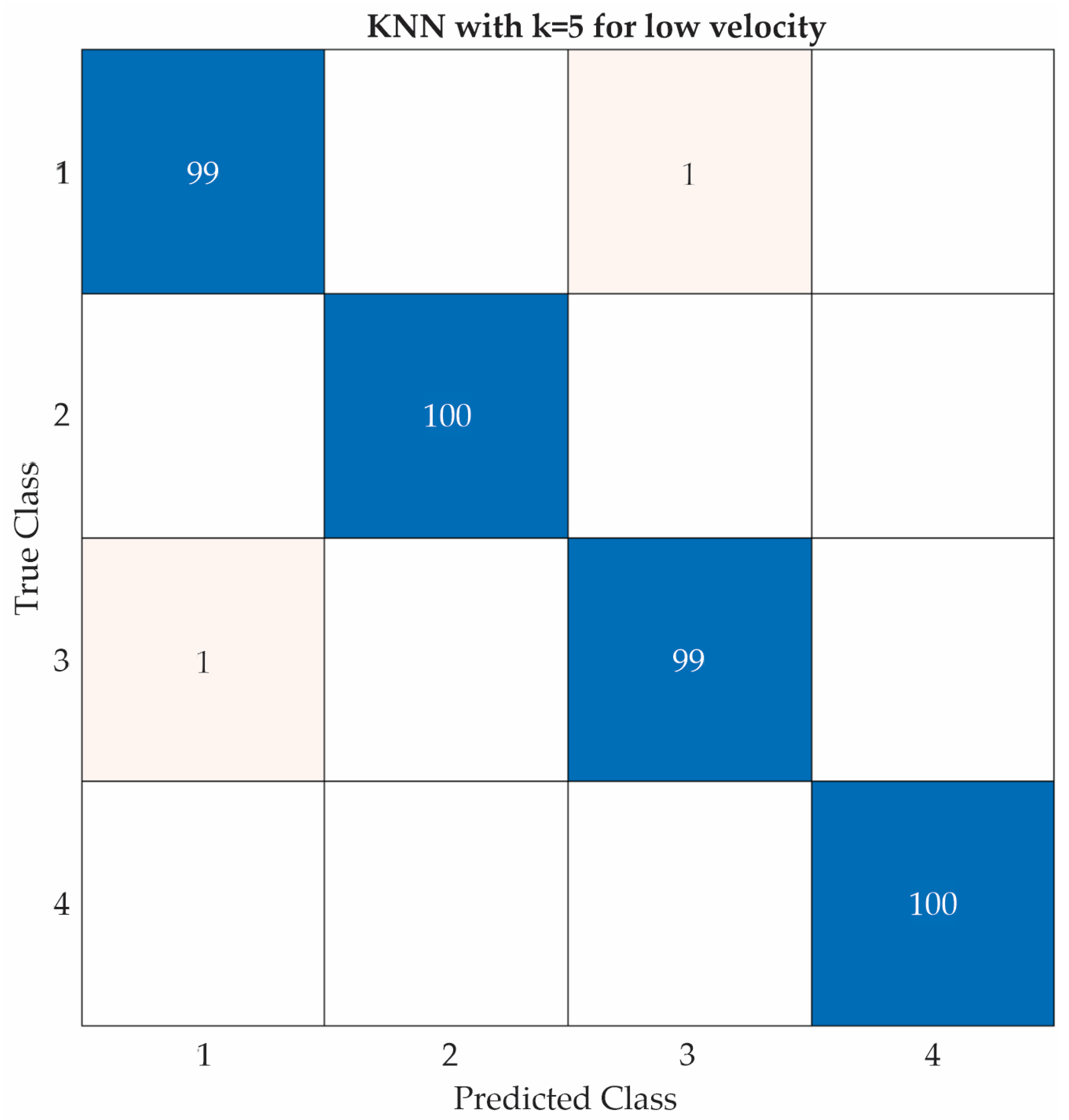
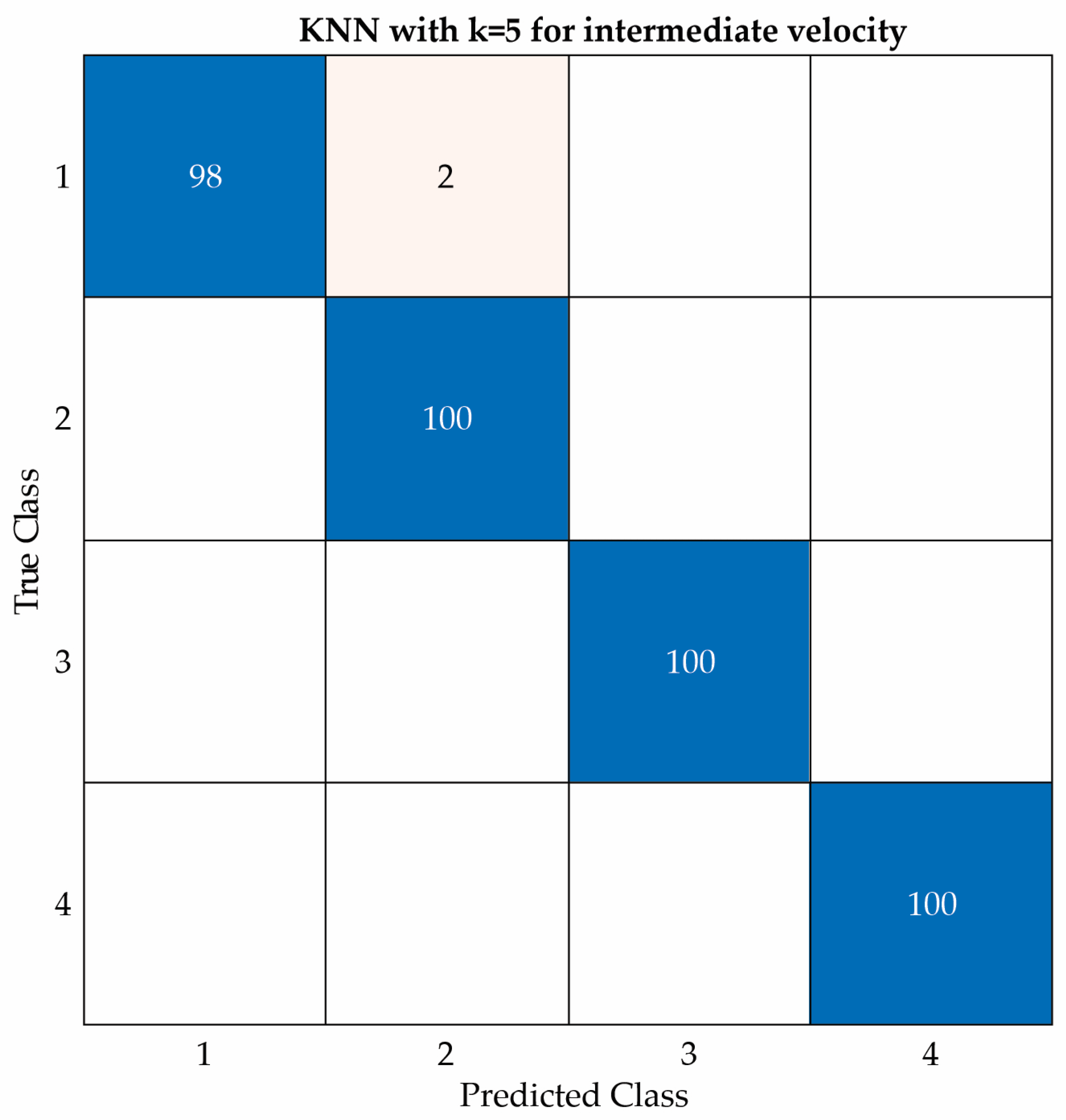
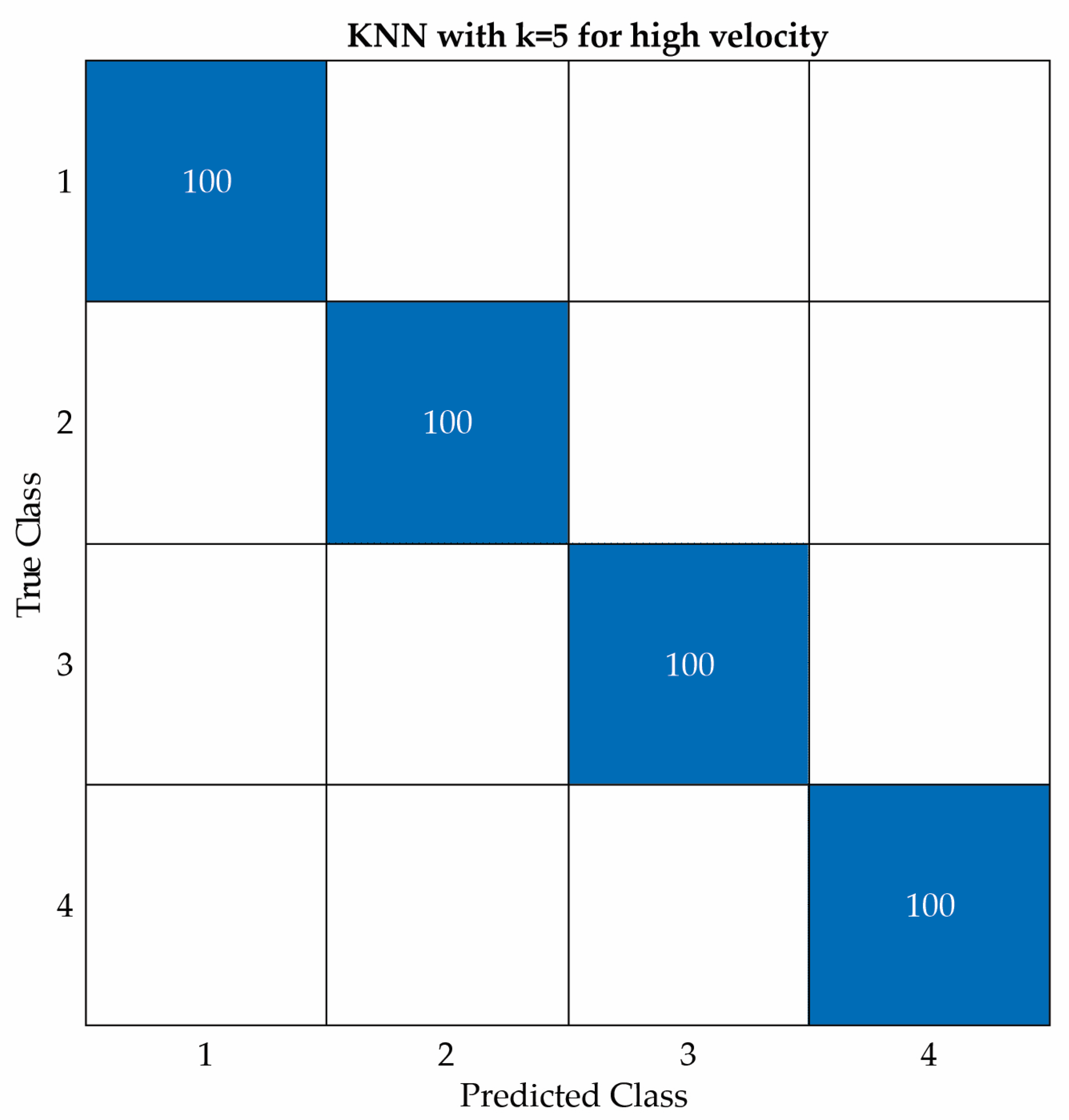
| Accuracy | 99.5% | 99.5% | 100% |
| Prediction speed | 8500 observation/s | 12,000 observation/s | 8400 observation/s |
| Training time | 18.253 s | 18.785 s | 21.945 s |
| Distance metric | Euclidean | Euclidean | Euclidean |
| Distance weight | Equal | Equal | Equal |
| Low Velocity | Intermediate Velocity | High Velocity | |||
|---|---|---|---|---|---|
| Feature | One-Way ANOVA | Feature | One-Way ANOVA | Feature | One-Way ANOVA |
| AxisY/Mean | 45.898 | AxisZ/Mean | 18.0144 | AxisY/RMS | 1.41 × 10³ |
| AxisY/Skewness | 28.7428 | AxisZ/RMS | 13.3412 | AxisY/Std | 563.3356 |
| AxisY/RMS | 26.7202 | AxisY/Mean | 5.2677 | AxisY/Mean | 329.2885 |
| AxisY/Std | 24.4612 | AxisY/Skewness | 3.1481 | AxisY/ShapeFactor | 226.6165 |
| AxisZ/Mean | 22.4664 | AxisY/PeakValue | 2.4873 | AxisY/PeakValue | 214.3894 |
| AxisY/SINAD | 19.7261 | AxisZ/Std | 2.2055 | AxisX/SNR | 58.6886 |
| AxisZ/RMS | 18.9073 | AxisZ/ShapeFactor | 2.1075 | AxisX/ShapeFactor | 57.6459 |
| AxisZ/ShapeFactor | 16.2734 | AxisY/Kurtosis | 2.054 | AxisY/ClearanceFactor | 51.9998 |
| AxisZ/SNR | 15.4659 | AxisY/RMS | 1.9922 | AxisZ/RMS | 50.3171 |
| AxisZ/Std | 15.0407 | AxisY/Std | 1.9866 | AxisX/Std | 47.4861 |
Disclaimer/Publisher’s Note: The statements, opinions and data contained in all publications are solely those of the individual author(s) and contributor(s) and not of MDPI and/or the editor(s). MDPI and/or the editor(s) disclaim responsibility for any injury to people or property resulting from any ideas, methods, instructions or products referred to in the content. |
© 2023 by the authors. Licensee MDPI, Basel, Switzerland. This article is an open access article distributed under the terms and conditions of the Creative Commons Attribution (CC BY) license (https://creativecommons.org/licenses/by/4.0/).
Share and Cite
Rangel-Rodriguez, A.H.; Granados-Lieberman, D.; Amezquita-Sanchez, J.P.; Bueno-Lopez, M.; Valtierra-Rodriguez, M. Analysis of Vibration Signals Based on Machine Learning for Crack Detection in a Low-Power Wind Turbine. Entropy 2023, 25, 1188. https://doi.org/10.3390/e25081188
Rangel-Rodriguez AH, Granados-Lieberman D, Amezquita-Sanchez JP, Bueno-Lopez M, Valtierra-Rodriguez M. Analysis of Vibration Signals Based on Machine Learning for Crack Detection in a Low-Power Wind Turbine. Entropy. 2023; 25(8):1188. https://doi.org/10.3390/e25081188
Chicago/Turabian StyleRangel-Rodriguez, Angel H., David Granados-Lieberman, Juan P. Amezquita-Sanchez, Maximiliano Bueno-Lopez, and Martin Valtierra-Rodriguez. 2023. "Analysis of Vibration Signals Based on Machine Learning for Crack Detection in a Low-Power Wind Turbine" Entropy 25, no. 8: 1188. https://doi.org/10.3390/e25081188