
Critic Learning-Based Safe Optimal Control for Nonlinear Systems with Asymmetric Input Constraints and Unmatched Disturbances


Abstract
:1. Introduction
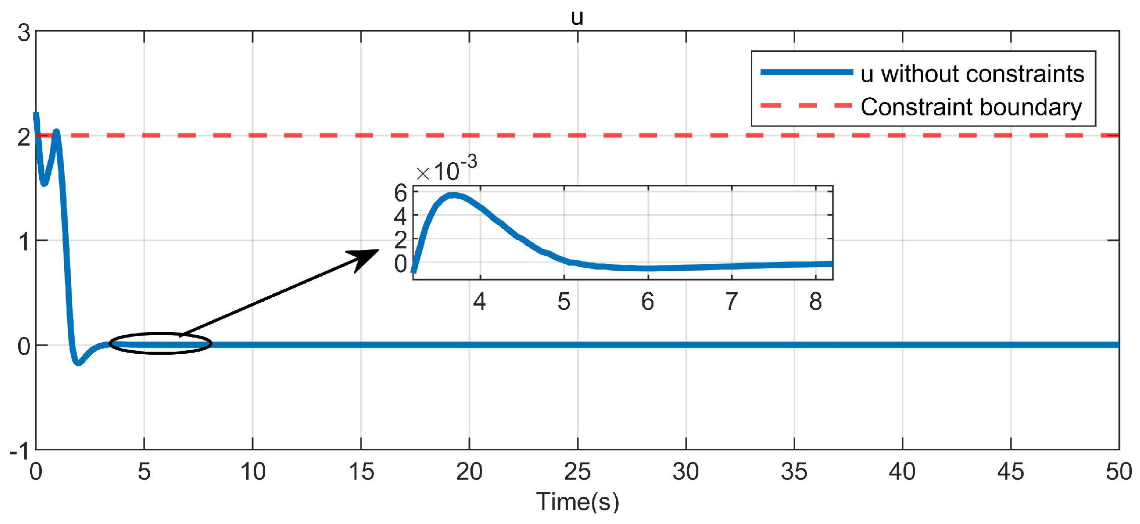
- Asymmetric input constraints are considered in the control problem of the CT nonlinear safety-critical systems. In addition, this paper proposes a new non-quadratic form function to address the issue of asymmetric input constraints. It is important to note that when applying this approach, the optimal control policy no longer remains at 0, even when the system state reaches the equilibrium point of (see in later Equation (15)).
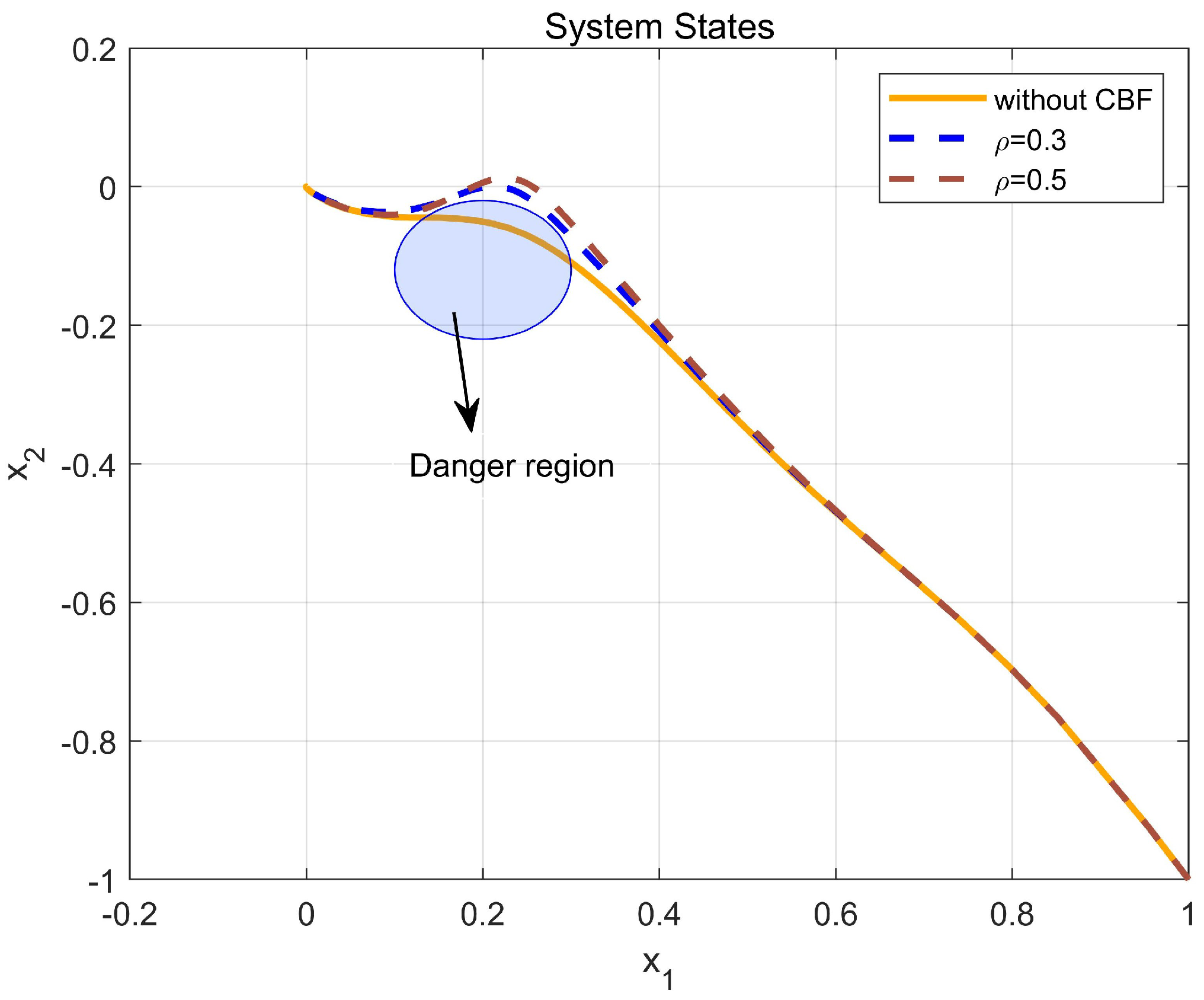
- This paper adopts the CBF to construct safety constraints and proposes designing a damping coefficient within the CBF to balance the safety and optimality of safety-critical systems based on varying safety requirements in different applications.
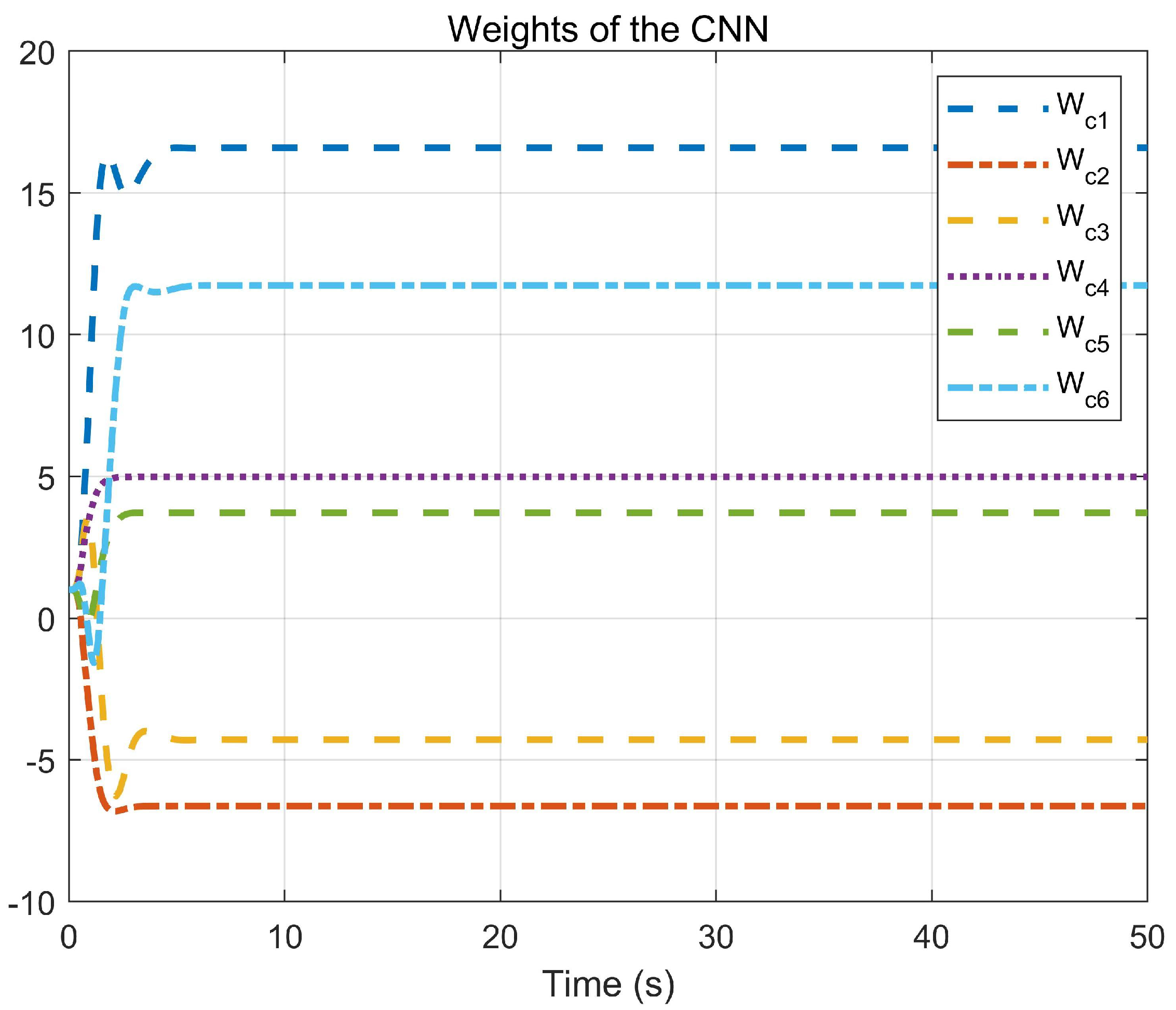
- The safe optimal control problem is turned into the ZSG problem to address unmatched disturbances; then, the optimal control law is gained by tackling the HJI equation using one CNN. Moreover, the use of only one CNN to approximate the HJI equation is an effective way to reduce the computational burden compared to the actor–critic network and the system state, and CNN parameters are demonstrated to be UUB.
2. Problem Statement
3. Safe Optimal Control Design
3.1. Control Barrier Function
- (1)
- ,
- (2)
- ,
- (3)
- is monotonically decreasing .
3.2. Safe and Optimal Control Approach
4. Adaptive CNN Design
4.1. Solving the HJI Equation via the CNN
4.2. Stability Analysis
- (1)
- for any .
- (2)
- for any .
- (3)
- for any .
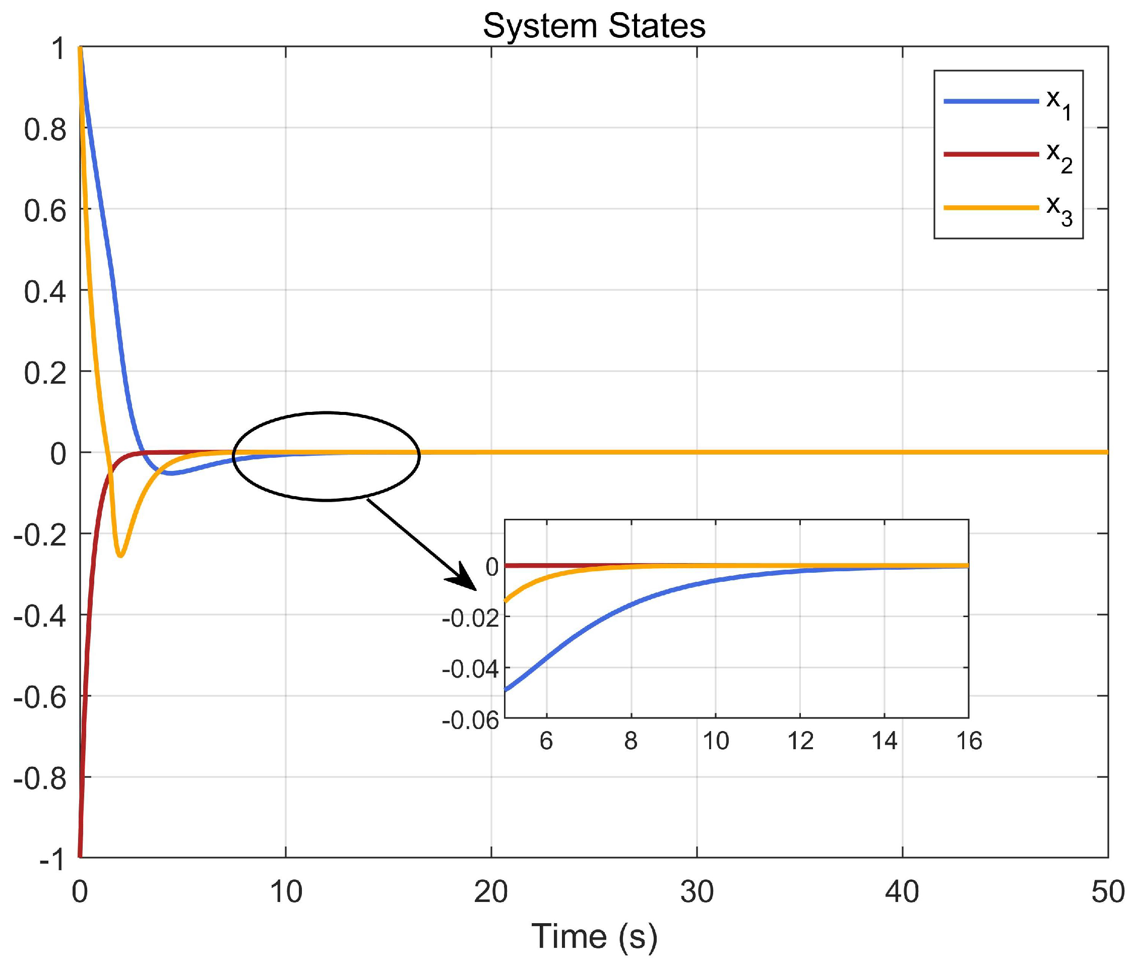
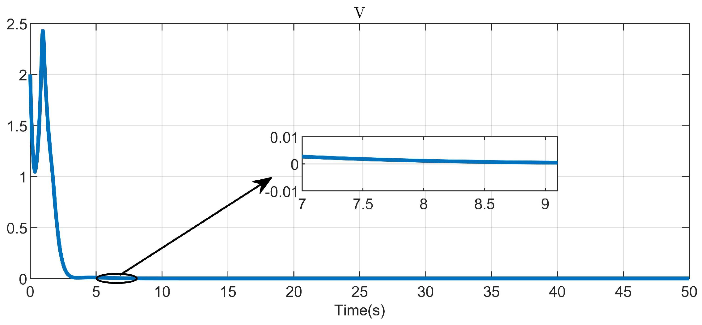
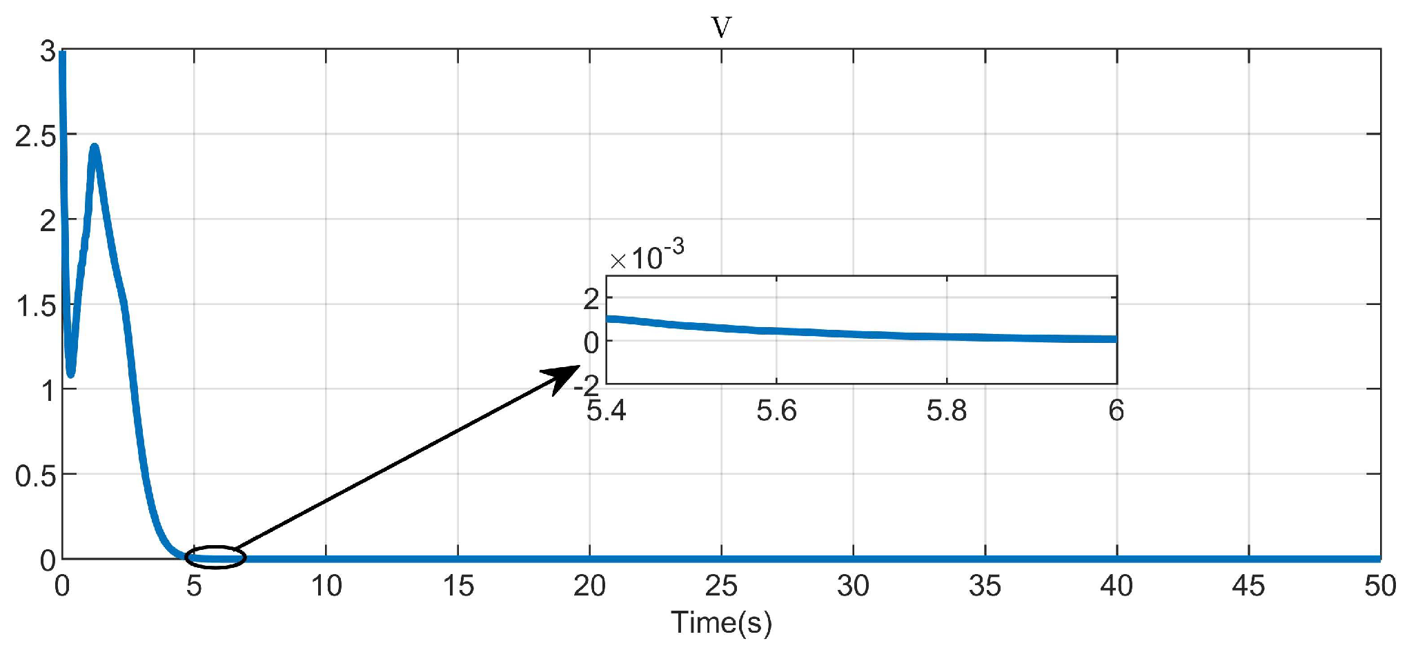
5. Simulation Study
5.1. Example 1
5.2. Example 2
6. Conclusions
Author Contributions
Funding
Institutional Review Board Statement
Data Availability Statement
Conflicts of Interest
References
- Yi, X.; Luo, B.; Zhao, Y. Adaptive dynamic programming-based visual servoing control for quadrotor. Neurocomputing 2022, 504, 251–261. [Google Scholar] [CrossRef]
- Liscouët, J.; Pollet, F.; Jézégou, J.; Budinger, M.; Delbecq, S.; Moschetta, J. A methodology to integrate reliability into the conceptual design of safety-critical multirotor unmanned aerial vehicles. Aerosp. Sci. Technol. 2022, 127, 107681. [Google Scholar] [CrossRef]
- Dou, L.; Cai, S.; Zhang, X.; Su, X.; Zhang, R. Event-triggered-based adaptive dynamic programming for distributed formation control of multi-UAV. J. Frankl. Inst. 2022, 359, 3671–3691. [Google Scholar] [CrossRef]
- Molnar, T.; Cosner, R.; Singletary, A.; Ubellacker, W.; Ames, A. Model-free safety-critical control for robotic systems. IEEE Robot. Autom. Lett. 2021, 7, 944–951. [Google Scholar] [CrossRef]
- Nguyen, Q.; Sreenath, K. Robust safety-critical control for dynamic robotics. IEEE Trans. Autom. Control 2021, 67, 1073–1088. [Google Scholar] [CrossRef]
- Liu, S.; Liu, L.; Yu, Z. Safe reinforcement learning for affine nonlinear systems with state constraints and input saturation using control barrier functions. Neurocomputing 2023, 518, 562–576. [Google Scholar] [CrossRef]
- Han, J.; Liu, X.; Wei, X.; Sun, S. A dynamic proportional-integral observer-based nonlinear fault-tolerant controller design for nonlinear system with partially unknown dynamic. IEEE Trans. Syst. Man Cybern. Syst. 2021, 52, 5092–5104. [Google Scholar] [CrossRef]
- Ohnishi, M.; Wang, L.; Notomista, G.; Egerstedt, M. Barrier-certified adaptive reinforcement learning with applications to brushbot navigation. IEEE Trans. Robot. 2019, 35, 1186–1205. [Google Scholar] [CrossRef] [Green Version]
- Bianchi, D.; Di Gennaro, S.; Di Ferdinando, M.; Acosta Lùa, C. Robust Control of UAV with Disturbances and Uncertainty Estimation. Machines 2023, 11, 352. [Google Scholar] [CrossRef]
- Bianchi, D.; Borri, A.; Di Benedetto, M.; Di Gennaro, S. Active Attitude Control of Ground Vehicles with Partially Unknown Model. IFAC-PapersOnLine 2020, 53, 14420–14425. [Google Scholar] [CrossRef]
- Ames, A.; Xu, X.; Grizzle, J.; Tabuada, P. Control barrier function based quadratic programs for safety critical systems. IEEE Trans. Autom. Control 2016, 62, 3861–3876. [Google Scholar] [CrossRef]
- Wang, H.; Peng, J.; Zhang, F.; Zhang, H.; Wang, Y. High-order control barrier functions-based impedance control of a robotic manipulator with time-varying output constraints. ISA Trans. 2022, 129, 361–369. [Google Scholar] [CrossRef] [PubMed]
- Liu, S.; Liu, L.; Yu, Z. Safe reinforcement learning for discrete-time fully cooperative games with partial state and control constraints using control barrier functions. Neurocomputing 2023, 517, 118–132. [Google Scholar] [CrossRef]
- Qin, C.; Wang, J.; Zhu, H.; Zhang, J.; Hu, S.; Zhang, D. Neural network-based safe optimal robust control for affine nonlinear systems with unmatched disturbances. Neurocomputing 2022, 506, 228–239. [Google Scholar] [CrossRef]
- Xu, X.; Tabuada, P.; Grizzle, J.W.; Ames, A. Robustness of control barrier functions for safety critical control. IFAC-PapersOnLine 2015, 48, 54–61. [Google Scholar] [CrossRef]
- Marvi, Z.; Kiumarsi, B. Safe reinforcement learning: A control barrier function optimization approach. Int. J. Robust Nonlinear Control 2021, 31, 1923–1940. [Google Scholar] [CrossRef]
- Xiao, W.; Belta, C.; Cassandras, C. Adaptive control barrier functions. IEEE Trans. Autom. Control 2021, 67, 2267–2281. [Google Scholar] [CrossRef]
- Modares, H.; Lewis, F.; Sistani, M. Online solution of nonquadratic two-player zero-sum games arising in the H∞ control of constrained input systems. Int. J. Adapt. Control Signal Process. 2014, 28, 232–254. [Google Scholar] [CrossRef]
- Qin, C.; Zhu, H.; Wang, J.; Xiao, Q.; Zhang, D. Event-triggered safe control for the zero-sum game of nonlinear safety-critical systems with input saturation. IEEE Access 2022, 10, 40324–40337. [Google Scholar] [CrossRef]
- Song, R.; Zhu, L. Stable value iteration for two-player zero-sum game of discrete-time nonlinear systems based on adaptive dynamic programming. Neurocomputing 2019, 340, 180–195. [Google Scholar] [CrossRef]
- Lu, W.; Li, Q.; Lu, K.; Lu, Y.; Guo, L.; Yan, W.; Xu, F. Load adaptive PMSM drive system based on an improved ADRC for manipulator joint. IEEE Access 2021, 9, 33369–33384. [Google Scholar] [CrossRef]
- Qin, C.; Qiao, X.; Wang, J.; Zhang, D. Robust Trajectory Tracking Control for Continuous-Time Nonlinear Systems with State Constraints and Uncertain Disturbances. Entropy 2022, 24, 816. [Google Scholar] [CrossRef] [PubMed]
- Fan, Q.; Yang, G. Adaptive actor—Critic design-based integral sliding-mode control for partially unknown nonlinear systems with input disturbances. IEEE Trans. Neural Netw. Learn. Syst. 2015, 27, 165–177. [Google Scholar] [CrossRef]
- Yang, X.; He, H. Event-driven H∞-constrained control using adaptive critic learning. IEEE Trans. Cybern. 2020, 51, 4860–4872. [Google Scholar] [CrossRef] [PubMed]
- Lewis, F.; Vrabie, D.; Syrmos, V. Optimal Control; John Wiley & Sons: Hoboken, NJ, USA, 2012. [Google Scholar]
- Kiumarsi, B.; Vamvoudakis, K.; Modares, H.; Lewis, F. Optimal and autonomous control using reinforcement learning: A survey. IEEE Trans. Neural Netw. Learn. Syst. 2017, 29, 2042–2062. [Google Scholar] [CrossRef]
- Liu, D.; Xue, S.; Zhao, B.; Luo, B.; Wei, Q. Adaptive dynamic programming for control: A survey and recent advances. IEEE Trans. Syst. Man Cybern. Syst. 2020, 51, 142–160. [Google Scholar] [CrossRef]
- Vamvoudakis, K.; Lewis, F. Online actor—Critic algorithm to solve the continuous-time infinite horizon optimal control problem. Automatica 2010, 46, 878–888. [Google Scholar] [CrossRef]
- Han, H.; Zhang, J.; Yang, H.; Hou, Y.; Qiao, J. Data-driven robust optimal control for nonlinear system with uncertain disturbances. Inf. Sci. 2023, 621, 248–264. [Google Scholar] [CrossRef]
- Lou, X.; Zhang, X.; Ye, Q. Robust control for uncertain impulsive systems with input constraints and external disturbance. Int. J. Robust Nonlinear Control 2022, 32, 2330–2343. [Google Scholar] [CrossRef]
- Wang, N.; Gao, Y.; Yang, C.; Zhang, X. Reinforcement learning-based finite-time tracking control of an unknown unmanned surface vehicle with input constraints. Neurocomputing 2022, 484, 26–37. [Google Scholar] [CrossRef]
- Liu, C.; Zhang, H.; Xiao, G.; Sun, S. Integral reinforcement learning based decentralized optimal tracking control of unknown nonlinear large-scale interconnected systems with constrained-input. Neurocomputing 2019, 323, 1–11. [Google Scholar] [CrossRef]
- Yang, X.; Zhao, B. Optimal neuro-control strategy for nonlinear systems with asymmetric input constraints. IEEE/CAA J. Autom. Sin. 2020, 7, 575–583. [Google Scholar] [CrossRef]
- Tang, Y.; Yang, X. Robust tracking control with reinforcement learning for nonlinear-constrained systems. Int. J. Robust Nonlinear Control 2022, 32, 9902–9919. [Google Scholar] [CrossRef]
- Zhou, W.; Liu, H.; He, H.; Yi, J.; Li, T. Neuro-optimal tracking control for continuous stirred tank reactor with input constraints. IEEE Trans. Ind. Inform. 2018, 15, 4516–4524. [Google Scholar] [CrossRef]
- Kong, L.; He, W.; Dong, Y.; Cheng, L.; Yang, C.; Li, Z. Asymmetric bounded neural control for an uncertain robot by state feedback and output feedback. IEEE Trans. Syst. Man Cybern. Syst. 2019, 51, 1735–1746. [Google Scholar] [CrossRef] [Green Version]
- Zhang, Y.; Zhao, B.; Liu, D.; Zhang, S. Event-triggered control of discrete-time zero-sum games via deterministic policy gradient adaptive dynamic programming. IEEE Trans. Syst. Man Cybern. Syst. 2021, 52, 4823–4835. [Google Scholar] [CrossRef]
- Zhang, S.; Zhao, B.; Liu, D.; Zhang, Y. Observer-based event-triggered control for zero-sum games of input constrained multi-player nonlinear systems. Neural Netw. 2021, 144, 101–112. [Google Scholar] [CrossRef]
- Wei, Q.; Liu, D.; Lin, Q.; Song, R. Adaptive dynamic programming for discrete-time zero-sum games. IEEE Trans. Neural Networks Learn. Syst. 2017, 29, 957–969. [Google Scholar] [CrossRef]
- Perrusquía, A.; Yu, W. Continuous-time reinforcement learning for robust control under worst-case uncertainty. Int. J. Syst. Sci. 2021, 52, 770–784. [Google Scholar] [CrossRef]
- Yang, Y.; Vamvoudakis, K.; Modares, H.; Yin, Y.; Wunsch, D. Safe intermittent reinforcement learning with static and dynamic event generators. IEEE Trans. Neural Netw. Learn. Syst. 2020, 31, 5441–5455. [Google Scholar] [CrossRef]
- Fu, Z.; Xie, W.; Rakheja, S.; Na, J. Observer-based adaptive optimal control for unknown singularly perturbed nonlinear systems with input constraints. IEEE/CAA J. Autom. Sin. 2017, 4, 48–57. [Google Scholar] [CrossRef]


Disclaimer/Publisher’s Note: The statements, opinions and data contained in all publications are solely those of the individual author(s) and contributor(s) and not of MDPI and/or the editor(s). MDPI and/or the editor(s) disclaim responsibility for any injury to people or property resulting from any ideas, methods, instructions or products referred to in the content. |
© 2023 by the authors. Licensee MDPI, Basel, Switzerland. This article is an open access article distributed under the terms and conditions of the Creative Commons Attribution (CC BY) license (https://creativecommons.org/licenses/by/4.0/).
Share and Cite
Qin, C.; Jiang, K.; Zhang, J.; Zhu, T. Critic Learning-Based Safe Optimal Control for Nonlinear Systems with Asymmetric Input Constraints and Unmatched Disturbances. Entropy 2023, 25, 1101. https://doi.org/10.3390/e25071101
Qin C, Jiang K, Zhang J, Zhu T. Critic Learning-Based Safe Optimal Control for Nonlinear Systems with Asymmetric Input Constraints and Unmatched Disturbances. Entropy. 2023; 25(7):1101. https://doi.org/10.3390/e25071101
Chicago/Turabian StyleQin, Chunbin, Kaijun Jiang, Jishi Zhang, and Tianzeng Zhu. 2023. "Critic Learning-Based Safe Optimal Control for Nonlinear Systems with Asymmetric Input Constraints and Unmatched Disturbances" Entropy 25, no. 7: 1101. https://doi.org/10.3390/e25071101