
Design and Analysis of Systematic Batched Network Codes


Abstract
:1. Introduction
1.1. Contributions Regarding Systematic Outer Codes
1.2. Contributions Regarding Inner Codes
1.3. Paper Organization
2. Ordinary Batched Network Coding
2.1. BATS Outer Code
- active packets that include a subset of the message packets and all the LDPC packets, and
- inactive packets that include all the other message packets and all the HDPC packets.
- Independently sample and obtain an integer , which is called the active degree of the batch;
- Uniformly, at random, choose active packets to be included in .
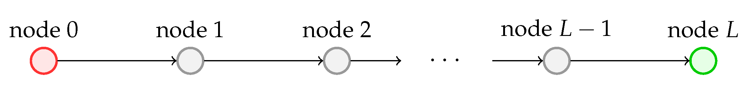
2.2. General Inner Code Formulation
2.3. Decoding Algorithms
2.3.1. Two-Step Decoding
- A batch i is said to be decodable if ; solve a decodable batch by Gaussian elimination;
- Substitute the decoded (precoded) packets into other undecoded batches and update the corresponding batch degree and generator matrix.
2.3.2. Joint Decoding
2.3.3. Inactivation Decoding
3. Systematic Outer Codes
3.1. Naive Approaches
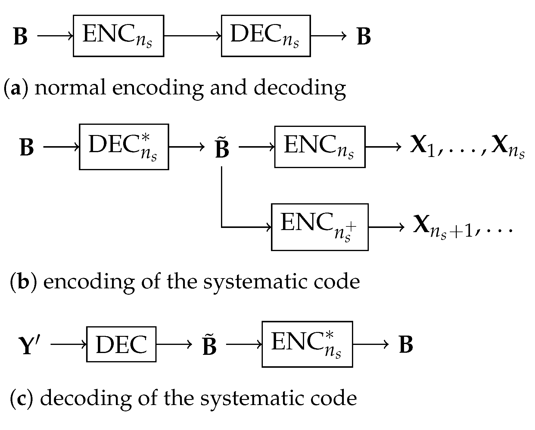
3.2. General Approach to Systematic Outer Codes
- and are deterministic; and
- for any K packets ,
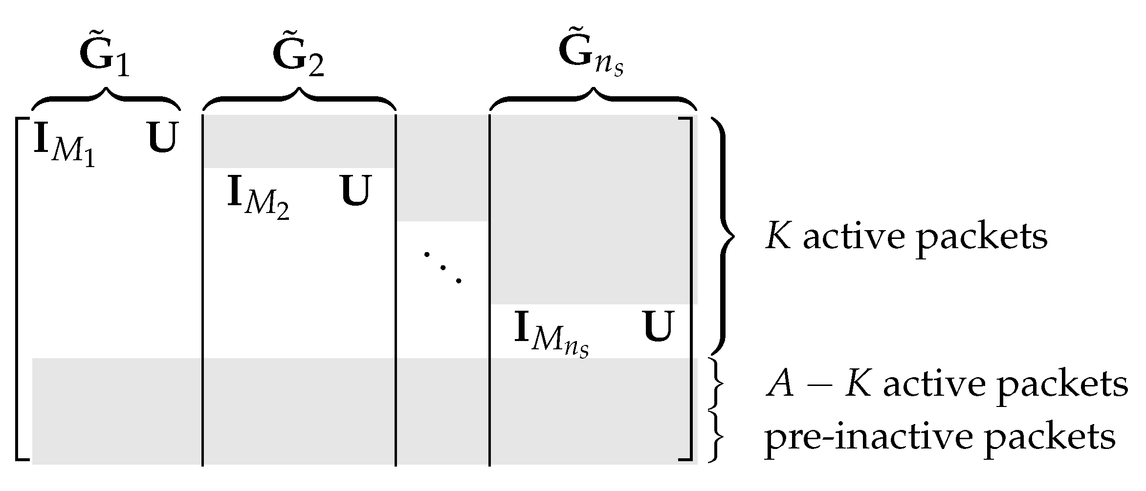
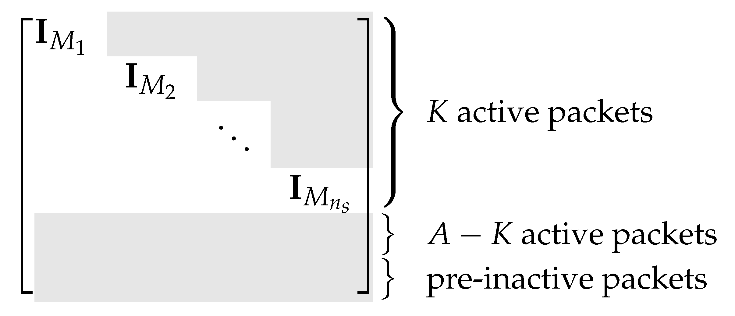
- Partition the message packets into subsets , , where the number of packets in the ith subset is ;
- Calculate ;
- Generate the first batches ;
- Generate more batches by performing on .
3.3. Computation Cost
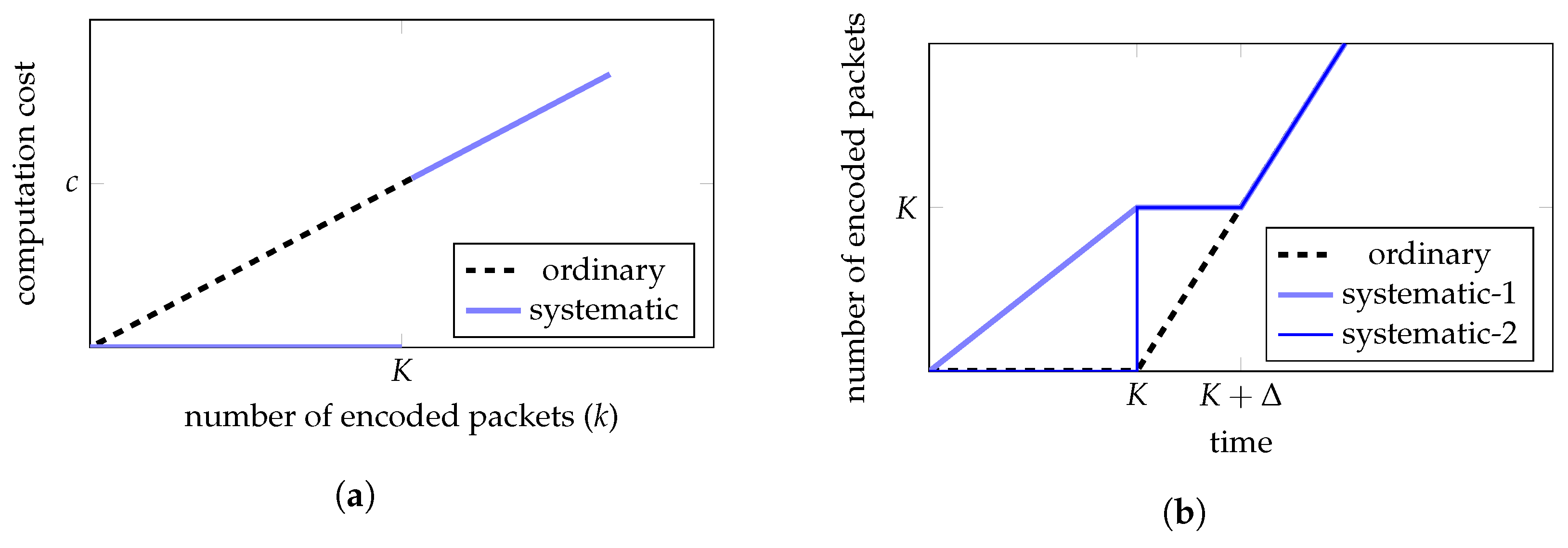
3.3.1. Encoding Computation Cost
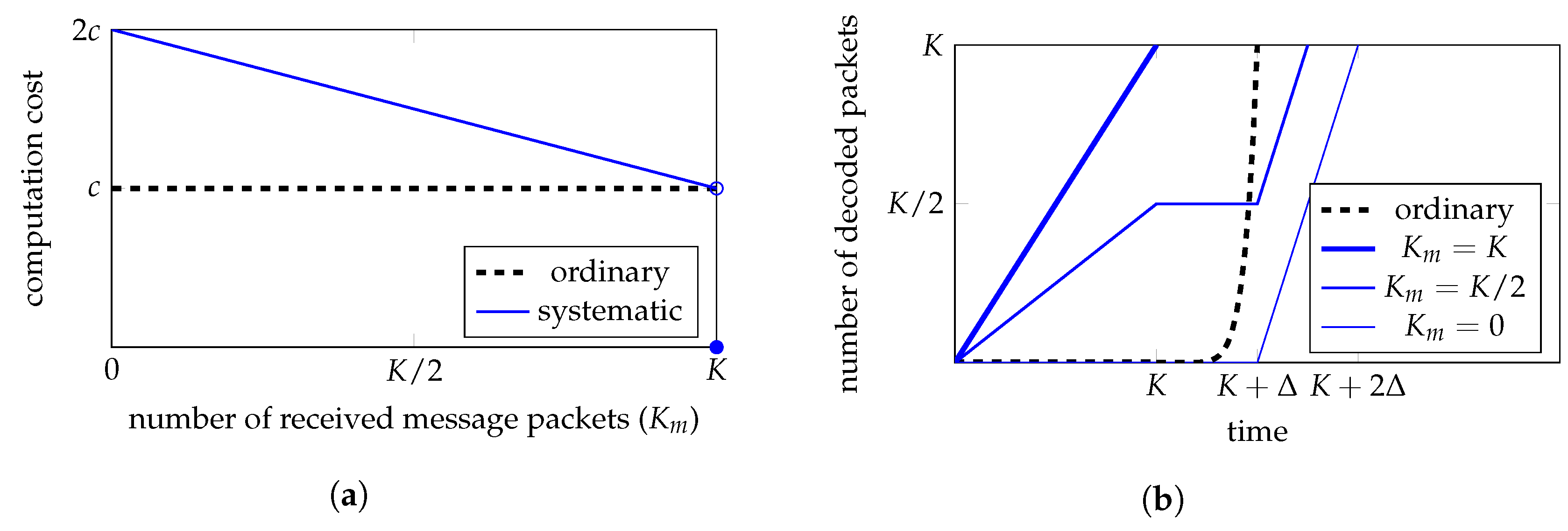
3.3.2. Decoding Computation Cost
3.4. Random Design
4. Triangular Embedding: A Structured Systematic Outer Code Design
4.1. Triangular Embedding Design
- the th to the th active packets, and
- a set of packets chosen from the first active packets and the last active packets.
4.2. Decoder Design
- First, inactivate all the packets used by the first batches among the last active packets;
- Second, apply belief propagation decoding to solve all the batches;
- Last, solve the inactive packets.
4.3. Design Verification
5. Inner Code for Systematic Batches
5.1. Detailed Inner Code Formulation
- When using RLIC for systematic batches, the probability that a recoded packet (a column of ) is a message packet is .
- When using SIC for systematic batches, if the network links have no packet loss, the destination node receives all the message packets without decoding. If each link has an erasure probability independently, the number of received message packets at the destination node drops exponentially rapidly with L increasing.
5.2. Recovery of Individual Message Packets
- The ith packet in has a unique solution;
- All the vectors such that (called the left nullspace collectively) have the ith entry 0;
- is orthogonal to the left nullspace of ;
- is in the column space of . □
5.3. Side Information for Message Packet Recovery
5.4. Recoding with Message Packet Protection
- Message Protection Recoding
- Systematic Message Protection Recoding
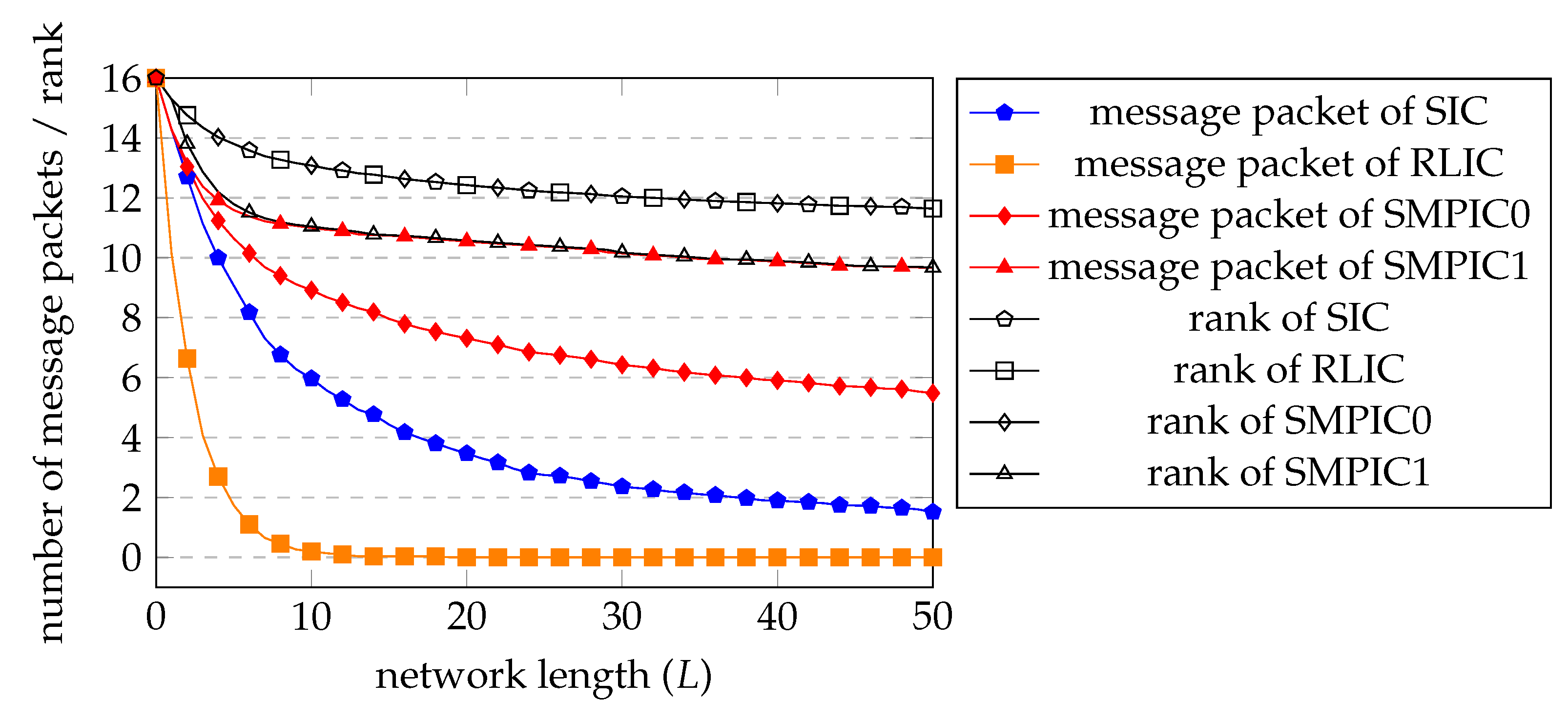
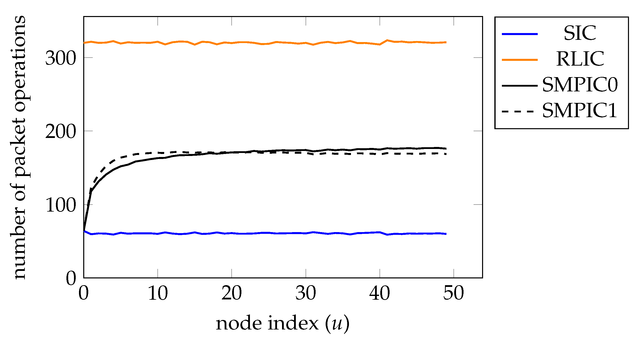
5.5. Numerical Evaluations
- SIC and RLIC have almost the same rank performance. SIC has a larger number of recoverable message packets than RLIC. However, for both SIC and RLIC, the number of recoverable message packets drops quickly.
- SMPIC0 has similar rank performance to SIC and RLIC and has a much higher average number of recoverable message packets than that of SIC and RLIC.
- SMPIC1 has the highest average number of recoverable message packets among the four inner codes, at the cost of a reduced average rank.
6. Concluding Remarks
7. Patents
- CN115811381A
- The design framework of the systematic BATS code (including the outer code and inner code), invented by the authors of this paper, published on 17 March 2023.
- CN2023105394085
- The design of the triangular embedded outer code, invented by L.M. and S.Y., filed on 15 May 2023.
Author Contributions
Funding
Institutional Review Board Statement
Data Availability Statement
Acknowledgments
Conflicts of Interest
Abbreviations
| BATS code | BATched Sparse code |
| HDPC | High-Density Parity Check |
| LDPC | Low-Density Parity Check |
| LCO | Linear Combination Operation |
| MPIC | Message Protection Inner Code |
| RLIC | Random Linear Inner Code |
| RLNC | Random Linear Network Codes/Random Linear Network Coding |
| SIC | Systematic Inner Code |
| SMPIC | Systematic Message Protection Inner Code |
Appendix A. Proofs Regarding Recoverability of Message Packets
Appendix B. BATS Code Parameters Used in Numerical Experiments
- The batch size M is 16.
- We use the degree distribution asymptotically optimized for the rank-M rank distribution. The non-zero entries of are listed in Table A1.
- The following formula determines the number of LDPC packets:
- The number of HDPC packets is .
- The decoder has a limit on the number of inactivated packets and the limit is 150.

| 0.0588 | 0.0571 | 0.0245 | 0.0899 | 0.1170 | 0.0921 | 0.0678 | 0.0679 |
| 0.0608 | 0.0604 | 0.0671 | 0.0671 | 0.0599 | 0.0222 | 0.0457 |
Appendix C. Pseudocodes for BATS Outer Encoding and Decoding
| Algorithm A1: The encoding process of the BATS outer code. |
Input:
Output:
|
| Algorithm A2: The two-step decoding process of the BATS outer code. |
Input:
Output:
|
References
- Ahlswede, R.; Cai, N.; Li, S.Y.R.; Yeung, R.W. Network information flow. IEEE Trans. Inform. Theory 2000, 46, 1204–1216. [Google Scholar] [CrossRef]
- Li, S.Y.R.; Yeung, R.W.; Cai, N. Linear network coding. IEEE Trans. Inform. Theory 2003, 49, 371–381. [Google Scholar] [CrossRef] [Green Version]
- Koetter, R.; Medard, M. An Algebraic Approach to Network Coding. IEEE/ACM Trans. Netw. 2003, 11, 782–795. [Google Scholar] [CrossRef] [Green Version]
- Ho, T.; Leong, B.; Medard, M.; Koetter, R.; Chang, Y.; Effros, M. The benefits of coding over routing in a randomized setting. In Proceedings of the IEEE International Symposium on Information Theory (ISIT ’03), Yokohama, Japan, 29 June–4 July 2003. [Google Scholar] [CrossRef] [Green Version]
- Ho, T.; Médard, M.; Koetter, R.; Karger, D.R.; Effros, M.; Shi, J.; Leong, B. A Random Linear Network Coding Approach to Multicast. IEEE Trans. Inform. Theory 2006, 52, 4413–4430. [Google Scholar] [CrossRef] [Green Version]
- Jaggi, S.; Chou, P.A.; Jain, K. Low complexity optimal algebraic multicast codes. In Proceedings of the International Symposium on Information Theory (ISIT ’03), Yokohama, Japan, 29 June–4 July 2003. [Google Scholar]
- Sanders, P.; Egner, S.; Tolhuizen, L. Polynomial time algorithms for network information flow. In Proceedings of the Fifteenth Annual ACM Symposium on Parallel Algorithms and Architectures (SPAA ’03), San Diego, CA, USA, 7–9 June 2003; pp. 286–294. [Google Scholar]
- Wu, Y. A Trellis Connectivity Analysis of Random Linear Network Coding with Buffering. In Proceedings of the 2006 IEEE International Symposium on Information Theory, Seattle, WA, USA, 9–14 July 2006; pp. 768–772. [Google Scholar] [CrossRef]
- Dana, A.F.; Gowaikar, R.; Palanki, R.; Hassibi, B.; Effros, M. Capacity of wireless erasure networks. IEEE Trans. Inform. Theory 2006, 52, 789–804. [Google Scholar] [CrossRef] [Green Version]
- Yeung, R.W. Avalanche: A network coding analysis. Commun. Inf. Syst. 2007, 7, 353–358. [Google Scholar] [CrossRef] [Green Version]
- Chou, P.A.; Wu, Y.; Jain, K. Practical Network Coding. In Proceedings of the Allerton Conference on Communication, Control, and Computing, Monticello, IL, USA, 29 September–1 October 2004. Invited paper. [Google Scholar]
- de Alwis, C.; Kodikara Arachchi, H.; Fernando, A.; Kondoz, A. Towards minimising the coefficient vector overhead in random linear Network Coding. In Proceedings of the 2013 IEEE International Conference on Acoustics, Speech and Signal Processing, Vancouver, BC, Canada, 26–31 May 2013; pp. 5127–5131. [Google Scholar] [CrossRef]
- Silva, D. Minimum-overhead network coding in the short packet regime. In Proceedings of the 2012 International Symposium on Network Coding (NetCod), Cambridge, MA, USA, 29–30 June 2012; pp. 173–178. [Google Scholar] [CrossRef]
- Gligoroski, D.; Kralevska, K.; Øverby, H. Minimal header overhead for random linear network coding. In Proceedings of the 2015 IEEE International Conference on Communication Workshop (ICCW), London, UK, 8–12 June 2015; pp. 680–685. [Google Scholar] [CrossRef] [Green Version]
- Silva, D.; Zeng, W.; Kschischang, F.R. Sparse Network Coding with Overlapping Classes. In Proceedings of the 2009 Workshop on Network Coding, Theory, and Applications (NetCod ’09), Lausanne, Switzerland, 15–16 June 2009; pp. 74–79. [Google Scholar] [CrossRef] [Green Version]
- Heidarzadeh, A.; Banihashemi, A.H. Overlapped Chunked network coding. In Proceedings of the 2010 IEEE Information Theory Workshop on Information Theory (ITW ’10), Cairo, Egypt, 6–8 January 2010; pp. 1–5. [Google Scholar]
- Li, Y.; Soljanin, E.; Spasojevic, P. Effects of the Generation Size and Overlap on Throughput and Complexity in Randomized Linear Network Coding. IEEE Trans. Inform. Theory 2011, 57, 1111–1123. [Google Scholar] [CrossRef] [Green Version]
- Mahdaviani, K.; Ardakani, M.; Bagheri, H.; Tellambura, C. Gamma Codes: A low-overhead linear-complexity network coding solution. In Proceedings of the 2012 International Symposium on Network Coding (NetCod), Cambridge, MA, USA, 29–30 June 2012; pp. 125–130. [Google Scholar] [CrossRef]
- Yang, S.; Yeung, R.W. Batched Sparse Codes. IEEE Trans. Inform. Theory 2014, 60, 5322–5346. [Google Scholar] [CrossRef] [Green Version]
- Tang, B.; Yang, S.; Yin, Y.; Ye, B.; Lu, S. Expander Chunked Codes. EURASIP J. Adv. Signal Process. 2015, 2015, 106. [Google Scholar] [CrossRef] [Green Version]
- Tang, B.; Yang, S. An LDPC Approach for Chunked Network Codes. IEEE/ACM Trans. Netw. 2018, 26, 605–617. [Google Scholar] [CrossRef]
- Yang, S.; Yeung, R.W. Network Communication Protocol Design from the Perspective of Batched Network Coding. IEEE Commun. Mag. 2022, 60, 89–93. [Google Scholar] [CrossRef]
- Yang, S.; Yeung, R.W. BATS Codes: Theory and Practice; Synthesis Lectures on Communication Networks; Morgan & Claypool Publishers: Williston, VT, USA, 2017. [Google Scholar] [CrossRef]
- MacWilliams, F.; Sloane, N. The Theory of Error-Correcting Codes; North-Holland Publishing: Amsterdam, The Netherlands, 1978. [Google Scholar]
- Versfeld, D.J.; Ridley, J.N.; Ferreira, H.C.; Helberg, A.S. On systematic generator matrices for Reed–Solomon codes. IEEE Trans. Inform. Theory 2010, 56, 2549–2550. [Google Scholar] [CrossRef]
- Luby, M.; Shokrollahi, A.; Watson, M.; Stockhammer, T.; Minder, L. RaptorQ Forward Error Correction Scheme for Object Delivery–RFC 6330; Internet Engineering Task Force: Fremont, CA, USA, 2011. [Google Scholar]
- Arikan, E. Systematic polar coding. IEEE Commun. Lett. 2011, 15, 860–862. [Google Scholar] [CrossRef] [Green Version]
- Badr, A.; Khisti, A.; Tan, W.T.; Apostolopoulos, J. Perfecting Protection for Interactive Multimedia: A survey of forward error correction for low-delay interactive applications. IEEE Signal Process. Mag. 2017, 34, 95–113. [Google Scholar] [CrossRef]
- Garcia-Saavedra, A.; Karzand, M.; Leith, D.J. Low Delay Random Linear Coding and Scheduling Over Multiple Interfaces. IEEE Trans. Mob. Comput. 2017, 16, 3100–3114. [Google Scholar] [CrossRef] [Green Version]
- Li, Y.; Zhang, F.; Wang, J.; Quek, T.Q.S.; Wang, J. On Streaming Coding for Low-Latency Packet Transmissions Over Highly Lossy Links. IEEE Commun. Lett. 2020, 24, 1885–1889. [Google Scholar] [CrossRef]
- Prior, R.; Rodrigues, A. Systematic network coding for packet loss concealment in broadcast distribution. In Proceedings of the The International Conference on Information Networking 2011 (ICOIN2011), Kuala Lumpur, Malaysia, 26–28 January 2011; pp. 245–250. [Google Scholar] [CrossRef]
- Lucani, D.E.; Medard, M.; Stojanovic, M. On Coding for Delay—Network Coding for Time-Division Duplexing. IEEE Trans. Inform. Theory 2012, 58, 2330–2348. [Google Scholar] [CrossRef] [Green Version]
- Yu, M.; Aboutorab, N.; Sadeghi, P. From Instantly Decodable to Random Linear Network Coded Broadcast. IEEE Trans. Commun. 2014, 62, 3943–3955. [Google Scholar] [CrossRef]
- Gabriel, F.; Wunderlich, S.; Pandi, S.; Fitzek, F.H.P.; Reisslein, M. Caterpillar RLNC With Feedback (CRLNC-FB): Reducing Delay in Selective Repeat ARQ Through Coding. IEEE Access 2018, 6, 44787–44802. [Google Scholar] [CrossRef]
- Phung, C.V.; Engelmann, A.; Jukan, A. Error Correction with Systematic RLNC in Multi-Channel THz Communication Systems. In Proceedings of the 2020 43rd International Convention on Information, Communication and Electronic Technology (MIPRO), Opatija, Croatia, 28 September–2 October 2020; pp. 512–517. [Google Scholar] [CrossRef]
- Karetsi, F.; Papapetrou, E. A Low Complexity Network-Coded ARQ protocol for Ultra-Reliable Low Latency Communication. In Proceedings of the 2021 IEEE 22nd International Symposium on a World of Wireless, Mobile and Multimedia Networks (WoWMoM), Pisa, Italy, 7–11 June 2021; pp. 11–20. [Google Scholar] [CrossRef]
- Shokrollahi, A.; Luby, M. Raptor Codes. Found. Trends Commun. Inf. Theory 2011, 6, 213–322. [Google Scholar] [CrossRef]
- Tasdemir, E.; Tömösközi, M.; Cabrera, J.A.; Gabriel, F.; You, D.; Fitzek, F.H.P.; Reisslein, M. SpaRec: Sparse Systematic RLNC Recoding in Multi-Hop Networks. IEEE Access 2021, 9, 168567–168586. [Google Scholar] [CrossRef]
- Pandi, S.; Gabriel, F.; Cabrera, J.A.; Wunderlich, S.; Reisslein, M.; Fitzek, F.H.P. PACE: Redundancy Engineering in RLNC for Low-Latency Communication. IEEE Access 2017, 5, 20477–20493. [Google Scholar] [CrossRef]
- Wunderlich, S.; Gabriel, F.; Pandi, S.; Fitzek, F.H.P.; Reisslein, M. Caterpillar RLNC (CRLNC): A Practical Finite Sliding Window RLNC Approach. IEEE Access 2017, 5, 20183–20197. [Google Scholar] [CrossRef]
- Lucani, D.E.; Pedersen, M.V.; Ruano, D.; Sørensen, C.W.; Fitzek, F.H.P.; Heide, J.; Geil, O.; Nguyen, V.; Reisslein, M. Fulcrum: Flexible Network Coding for Heterogeneous Devices. IEEE Access 2018, 6, 77890–77910. [Google Scholar] [CrossRef]
- Nguyen, V.; Tasdemir, E.; Nguyen, G.T.; Lucani, D.E.; Fitzek, F.H.P.; Reisslein, M. DSEP Fulcrum: Dynamic Sparsity and Expansion Packets for Fulcrum Network Coding. IEEE Access 2020, 8, 78293–78314. [Google Scholar] [CrossRef]
- Tasdemir, E.; Nguyen, V.; Nguyen, G.T.; Fitzek, F.H.P.; Reisslein, M. FSW: Fulcrum sliding window coding for low-latency communication. IEEE Access 2022, 10, 54276–54290. [Google Scholar] [CrossRef]
- Compta, P.T.; Fitzek, F.H.P.; Lucani, D.E. Network Coding is the 5G Key Enabling Technology: Effects and Strategies to Manage Heterogeneous Packet Lengths. Trans. Emerg. Telecommun. Technol. 2015, 6, 46–55. [Google Scholar] [CrossRef]
- Yang, S. Simbats. 2015. Available online: https://github.com/shhyang/simbats (accessed on 10 June 2022).


| 0 | 4784 | 3552 | 836 | 4 | 0 |
| 1 | 173 | 175 | 50 | 0 | 0 |
| 2 | 34 | 113 | 53 | 0 | 0 |
| ≥3 | 9 | 1160 | 4061 | 4996 | 5000 |
| zero overhead | 4978 | 4983 | 4977 |
| max total inact. | 27 | 91 | 149 |
| Coding Overhead | |||||
|---|---|---|---|---|---|
| (a) | |||||
| 0 | 4982 | 4955 | 3446 | 3 | 0 |
| 18 | 26 | 69 | 0 | 0 | |
| 0 | 3 | 51 | 0 | 0 | |
| 0 | 16 | 1434 | 4997 | 5000 | |
| (b) | |||||
| 0 | 4983 | 4511 | 1037 | 17 | 0 |
| 17 | 73 | 31 | 0 | 0 | |
| 0 | 39 | 25 | 1 | 0 | |
| 0 | 377 | 3907 | 4982 | 5000 | |
| (c) | |||||
| 0 | 4987 | 4155 | 1823 | 5 | 0 |
| 13 | 107 | 101 | 1 | 0 | |
| 0 | 61 | 72 | 1 | 0 | |
| 0 | 677 | 3004 | 4993 | 5000 |
Disclaimer/Publisher’s Note: The statements, opinions and data contained in all publications are solely those of the individual author(s) and contributor(s) and not of MDPI and/or the editor(s). MDPI and/or the editor(s) disclaim responsibility for any injury to people or property resulting from any ideas, methods, instructions or products referred to in the content. |
© 2023 by the authors. Licensee MDPI, Basel, Switzerland. This article is an open access article distributed under the terms and conditions of the Creative Commons Attribution (CC BY) license (https://creativecommons.org/licenses/by/4.0/).
Share and Cite
Mao, L.; Yang, S.; Huang, X.; Dong, Y. Design and Analysis of Systematic Batched Network Codes. Entropy 2023, 25, 1055. https://doi.org/10.3390/e25071055
Mao L, Yang S, Huang X, Dong Y. Design and Analysis of Systematic Batched Network Codes. Entropy. 2023; 25(7):1055. https://doi.org/10.3390/e25071055
Chicago/Turabian StyleMao, Licheng, Shenghao Yang, Xuan Huang, and Yanyan Dong. 2023. "Design and Analysis of Systematic Batched Network Codes" Entropy 25, no. 7: 1055. https://doi.org/10.3390/e25071055