Construction of Optimal Frequency Hopping Sequence Set with Low-Hit-Zone

Abstract

In quasi-synchronous frequency-hopping multiple access (QS-FHMA) systems, low-hit-zone (LHZ) frequency-hopping sequence (FHS) sets have been well-applied to reduce mutual interference (MI). In this paper, we propose three constructions of LHZ FHS sets with new parameters via interleaving techniques. The obtained sequences can be verified that they are optimal with respect to the Peng–Fan–Lee bound.

1. Introduction

Frequency-hopping multiple-access (FHMA) is widely used in modern communication systems such as military radar communication systems, Bluetooth communication systems, and more [1,2,3]. Simultaneous transmission of data by multiple users on the same frequency leads to mutual interference (MI), which should be minimized to improve the quality and reliability of the communication. In addition to this, there exists a strong association between the Hamming correlation (HC) of the frequency hopping sequence (FHS) set and the level of the MI. Therefore, it is reasonable to prioritize the construction of FHS sets with a low HC for the significance of the HC in evaluating the performance of frequency hopping sequences (FHSs).

The value of the MI will be maintained at a low level at the zone around the origin between various users, and the low-hit-zone (LHZ) FHS sets will be employed in quasi-synchronous (QS) FHMA systems. Thus, the construction of the optimal LHZ FHS set with respect to the Peng–Fan–Lee bound is preferable to the construction of the optimal FHS set with respect to the Peng–Fan bound [4] in some respects.

Numerous optimal LHZ FHS sets have been found that satisfy the Peng–Fan–Lee bound [5]. Ma and Sun [6] constructed the first class of optimal LHZ FHS sets with respect to the Peng–Fan–Lee bound in 2010. Using the Cartesian, Chung et al. [7] provided a few constructions of the optimal LHZ FHS sets in 2013. By using the interleaving technique, Niu et al. [8,9] obtained various constructions of optimal LHZ FHS sets in 2012 and 2014. Cai et al. [10,11] obtained classes of optimal LHZ FHS sets with optimal partial HC properties in 2014 and 2015. Han et al. [12] and Wang et al. [13] constructed LHZ FHS sets with different parameters in 2016. Using the Cartesian, Zhou et al. [14,15] introduced some constructions of LHZ FHS sets in 2017. Ling et al. [16] obtained a class of optimal LHZ FHS sets in the next year. Niu et al. [17,18] constructed a new class of optimal LHZ FHS sets with large family sizes in 2019. In the same year, the construction by Han et al. [19] of a class of LHZ FHS sets with the optimal partial HC. Niu et al. [20,21] constructed classes of optimal FHS sets in 2020. In 2022, Zhou et al. [22] constructed four classes of LHZ FHS sets with optimal partial HC properties.

In this paper, we propose three constructions of LHZ FHS sets with new parameters by interleaving technique and the LHZ FHS sets are optimal with respect to the Peng–Fan–Lee bound. We make the following arrangement for the remaining portion of this paper. We introduced some notations and the bounds on the FHS set in Section 2. We described how the LHZ FHS set is constructed by using an interleaving technique in Section 3. Finally, we made a few concluding remarks in Section 4.

2. Preliminaries

Let $F=\{f_1,f_2,\cdots ,f_c\}$ be a set with c available frequency slots. A sequence $X={\left\{x_j\right\}}_{j=0}^{L-1}$ is called a FHS of length L over F for all $x_j$, $0\le j\le L-1$. For any two FHSs $X={\left\{x_j\right\}}_{j=0}^{L-1}$, $Y={\left\{y_j\right\}}_{j=0}^{L-1}$ of length L over F, their Hamming correlation function $H_{XY}\left(\tau \right)$ of sequences X and Y at delay time $\tau$ is defined by

$$\begin{array}{ccc}\hfill H_{XY}\left(\tau \right)& =& \sum _{j=0}^{L-1}h[x_j,y_{j+\tau }]0\le \tau \le L-1,\hfill \end{array}$$

where the subscript $j+\tau$ of the above equation needs to be modulo L, and $h[x_j,y_{j+\tau }]=1$ if $x_j=y_{j+\tau }$, and 0 otherwise.

For a sequence X, the Hamming autocorrelation of X can be defined as

$$\begin{array}{c}\hfill H_a\left(X\right)=\underset{1\le \tau \le L-1}{max}\left\{H_{XX}\left(\tau \right)\right\}.\end{array}$$

For any given FHS set $\mathcal{Q}$, the maximum Hamming autocorrelation (MHAC) $H_a\left(\mathcal{Q}\right)$, the maximum Hamming crosscorrelation (MHCC) $H_c\left(\mathcal{Q}\right)$ and the maximum Hamming correlation (MHC) of $\mathcal{Q}$ are, respectively, defined as

$$\begin{array}{c}\hfill H_m\left(\mathcal{Q}\right)=max\left\{H_a\left(\mathcal{Q}\right),H_c\left(\mathcal{Q}\right)\right\},\end{array}$$

$$\begin{array}{c}\hfill H_a\left(\mathcal{Q}\right)=\underset{1\le \tau \le L-1}{max}\{H_{XX}\left(\tau \right)\mid X\in \mathcal{Q}\},\end{array}$$

$$\begin{array}{c}\hfill H_c\left(\mathcal{Q}\right)=\underset{0\le \tau \le L-1}{max}\{H_{XY}\left(\tau \right)\mid X,Y\in \mathcal{Q},X\ne Y\}.\end{array}$$

In 2004, Peng and Fan proposed a lower bound for an FHS set as follows.

Lemma 1 

(Peng-Fan bound [4]). Let $\mathcal{Q}$ $(L,N,c,H_m\left(\mathcal{Q}\right))$ be a set, then we have

$$H_m\left(\mathcal{Q}\right)\ge \frac{(NL-c)L}{(NL-1)c},$$

where $(L,N,c,H_m\left(\mathcal{Q}\right))$ denotes a set of N FHSs of length L with size c, with the MHC $H_m\left(\mathcal{Q}\right)$.

If each parameter of the FHS set $\mathcal{Q}$ substituted into the above equation satisfies the equal sign case, the $\mathcal{Q}$ is said to be the optimal FHS set.

For any FHS set $\mathcal{Q}$, if $H_a\ge 0$, $H_c\ge 0$, the LHZ $Z_h$ of $\mathcal{Q}$ is defined as

$$\begin{array}{cc}& Z_h=min\left\{Z_{ah},Z_{ch}\right\},\hfill \\ & \mathrm{where}\hfill \\ & Z_{ah}=\underset{1\le \tau \le G}{max}\left\{G\mid H_{XX}\left(\tau \right)\le H_a,\forall X\in \mathcal{Q}\right\},\hfill \\ & Z_{ch}=\underset{0\le \tau \le G}{max}\left\{G\mid H_{XY}\left(\tau \right)\le H_c,\forall X,Y\in \mathcal{Q},X\ne Y\right\}.\hfill \end{array}$$

In 2006, Peng, Fan and Lee proposed a lower bound for the LHZ FHS set as follows.

Lemma 2 

(Peng–Fan–Lee bound [5]). Let $\mathcal{Q}(L,N,c,Z_h,H_m\left(\mathcal{Q}\right)$ be the LHZ FHS set. Then, for any positive integer Z, $0\le Z\le Z_h$, we have

$$H_m\left(\mathcal{Q}\right)\ge \frac{(NZ+N-c)L}{(NZ+N-1)c},$$

where $(L,N,c,Z_h,H_m\left(\mathcal{Q}\right))$ denotes a set of N FHSs of length L with size c, with the MHC $H_m\left(\mathcal{Q}\right)$ and the LHZ $Z_h$.

If each parameter of the LHZ FHS set $\mathcal{Q}$ substituted into the above equation satisfies the equal sign case, the $\mathcal{Q}$ is said to be the optimal LHZ FHS set.

3. Interleaving Technique of FHSs

Let $A=(a_0,a_1,\cdots ,a_{L-1})$ be a $(L,c,H_a\left(A\right))$ FHS, and $E=(e_0,e_1,\cdots ,e_{T-1})$ be a shift sequence of length T over a frequency slot set of size p, i.e., $e_i\in p$, $0\le i<T$. A matrix of $TL$ can be obtained through the sequences A and E in the following way.

$$\begin{array}{cc}\hfill \gamma =& \left(\begin{array}{cccc}{a}_{0+e_0}& a_{0+e_1}& \dots & a_{0+e_{T-1}}\\ a_{1+e_0}& a_{1+e_1}& \dots & a_{1+e_{T-1}}\\ ⋮& ⋮& \ddots & ⋮\\ a_{L-1+e_0}& a_{L-1+e_1}& \dots & a_{L-1+e_{T-1}}\end{array}\right)\hfill \\ \hfill =& \left(\begin{array}{cccc}{b}_0& b_1& \dots & b_{T-1}\\ b_T& b_{T+1}& \dots & b_{2T-1}\\ ⋮& ⋮& \ddots & ⋮\\ b_{T(L-1)}& b_{T(L-1)+1}& \dots & b_{TL-1}\end{array}\right).\hfill \end{array}$$

(1)

Reading each element of the matrix $\gamma$ by row, we have a sequence $B=(b_0,b_1,\cdots ,b_{TL-1})$ of length $TL$. Let B be called the interleaved sequence and E is called a shift sequence. The interleaved sequence B can be written as

$$B=I\left(L^{e_0}\left(A\right),L^{e_1}\left(A\right),\cdots ,L^{e_{T-1}}\left(A\right)\right),$$

where I is the interleaving operator and L is the shift operator.

Let $U=(u_0,u_1,\cdots ,u_{T-1})$ be another shift sequence over a frequency slot set of size p and $V=I\left(L^{u_0}\left(A\right),L^{u_1}\left(A\right),\cdots ,L^{u_{T-1}}\left(A\right)\right)$. Considering the shift factor, we can obtain $L^{\tau }\left(V\right)$, where $\tau =T{\tau }_1+{\tau }_2\left(0\le {\tau }_2<T,0\le {\tau }_1<L\right)$. By the matrix representation, $L^{\tau }\left(V\right)$ could be written as

$$\left(\begin{array}{cccccc}{a}_{u_{{\tau }_2}+{\tau }_1}& \dots & a_{u_{T-1}+{\tau }_1}& a_{u_0+{\tau }_1+1}& \dots & a_{u_{{\tau }_2-1}+{\tau }_1+1}\\ a_{u_{{\tau }_2}+{\tau }_1+1}& \dots & a_{u_{T-1}+{\tau }_1+1}& a_{u_0+{\tau }_1+2}& \dots & a_{u_{{\tau }_2-1}+{\tau }_1+2}\\ ⋮& \ddots & ⋮& ⋮& \ddots & ⋮\\ a_{u_{{\tau }_2}+{\tau }_1-1}& \dots & a_{u_{T-1}+{\tau }_1-1}& a_{u_0+{\tau }_1}& \dots & a_{u_{{\tau }_2-1}+{\tau }_1}\end{array}\right).$$

(2)

Obviously, $L^{\tau }\left(V\right)$ is just another interleaved sequence. Namely, we have

$$L^{\tau }\left(V\right)=I(L^{u_{{\tau }_2}+{\tau }_1}\left(A\right),\cdots ,L^{u_{T-1}+{\tau }_1}\left(A\right),L^{u_0+{\tau }_1+1}\left(A\right),\cdots ,L^{u_{{\tau }_2-1}+{\tau }_1+1}\left(A\right)).$$

Then, the obtained HC function of the interleaved sequence B and V at delay time $\tau$ can be expressed as the summation of the inner product between the (1) and (2). Then, we have

$$H_{BV}\left(\tau \right)=\sum _{t=0}^{T-{\tau }_2-1}{H}_{AA}\left(u_{t+{\tau }_2}-e_t+{\tau }_1\right)+\sum _{t=T-{\tau }_2}^{T-1}{H}_{AA}\left(u_{t+{\tau }_2-T}-e_t+{\tau }_1+1\right).$$

For any ${\tau }_2,0\le {\tau }_2<T$, let

$$d_{t,{\tau }_2}^{(E,U)}=\left\{\begin{array}{cc}{e}_t-u_{t+{\tau }_2},\hfill & 0\le t\le T-1-{\tau }_2\hfill \\ e_t-u_{t+{\tau }_2-T}-1,\hfill & T-{\tau }_2\le t\le T-1\hfill \end{array}\right.,$$

where $d_{t,{\tau }_2}^{(E,U)}$ needs to be modulo p. Then, the HC function of B and V can be rewritten as

$$H_{BV}\left(\tau \right)=\sum _{t=0}^{T-1}{H}_{AA}\left({\tau }_1-d_{t,{\tau }_2}^{(E,U)}\right).$$

Lemma 3. 

According to the above notation, for the sequences B and V, corresponding to the shift sequences E and U, we have

$$\begin{array}{cc}\hfill & H_{BV}\left(\tau \right)=T{H}_a,\mathrm{for}{\tau }_1<\underset{0\le t,{\tau }_2<T}{min}\left\{d_{t,{\tau }_2}^{(E,U)}\right\},\hfill \end{array}$$

where $\tau =T{\tau }_1+{\tau }_2\left(0\le {\tau }_2<T,0\le {\tau }_1<L\right).$

Besides, we introduce a class of construction methods by an interleaving technique as follows.

Step 1:

Select an $(L,N,c,H_m\left(\mathcal{A}\right))$ FHS set $\mathcal{A}$,

$$\mathcal{A}=\left\{a^i=\left(a_0^i,a_1^i,\cdots ,a_{L-1}^i\right)\mid 0\le i<N\right\}.$$

Step 2:

For a given T, and $gcd(L,T)=1$, generate a set of shift sequences,

$$\mathcal{E}=\left\{e^j=\left(e_0^j,e_1^j,\cdots ,e_{T-1}^j\right)\mid 0\le j<M\right\}.$$

Step 3:

Construct the FHS set $\mathcal{B}=\{b^k\mid 0\le k<NM\}$, where $k=iM+j(0\le j<M,0\le i<N)$. Then for any $0\le k<NM$,

$$b^k=I\left(L^{e_0^j}\left(a^i\right),L^{e_1^j}\left(a^i\right),\cdots ,L^{e_{T-1}^j}\left(a^i\right)\right).$$

By the above construction, we can deduce the LHZ and MHC of this LHZ FHS set as follows.

Theorem 1. 

The sequence set $\mathcal{B}=\{b^k\mid 0\le k<NM\}$ generated by the interleaving technique is a $(TL,NM,c,Z_h,T{H}_m\left(\mathcal{A}\right))$ LHZ FHS set, where

$$\begin{array}{cc}\hfill & Z_h+1=\hfill \\ \hfill & min\left\{\underset{e^{j_1}\in \mathcal{E}}{min}\left\{\underset{0\le t,{\tau }_2<T}{min}\left\{T{d}_{t,{\tau }_2}^{\left(e^{j_1},e^{j_1}\right)}+{\tau }_2\right\}\right\}\right.,\left.\underset{e^{j_1}\ne e^{j_2}\in \mathcal{E}}{min}\left\{\underset{\left(0\le t,{\tau }_2<T\right.}{min}\left\{T{d}_{t,{\tau }_2}^{\left(e^{j_1},e^{j_2}\right)}+{\tau }_2\right\}\right\}\right\}.\hfill \end{array}$$

Proof of Theorem 1. 

For any two FHSs $b^{k_1}$, $b^{k_2}$∈$\mathcal{B}$, which correspond to the shift sequences $e^{j_1}$ and $e^{j_2}$∈$\mathcal{E}$, then the MHC of $H_m\left(\mathcal{B}\right)$ in the LHZ can be verified as follows.

Case 1: $k_1=k_2$. Then we have $e^{j_1}$ = $e^{j_2}$. From Lemma 3, the MHAC of the sequences is $T{H}_a\left(\mathcal{A}\right)$, when $0<{\tau }_2\le {min}_{e^{j_1}\in \mathcal{E}}\left\{{min}_{0\le t,{\tau }_2<T}\left\{T{d}_{t,{\tau }_2}^{\left(e^{j_1},e^{j_1}\right)}+{\tau }_2\right\}\right\}$. The case does not need to be concerned when the ${\tau }_2=0$.

Case 2: $k_1\ne k_2$.

(1)

If $a^{i_1}\ne a^{i_2}$ and $e^{j_1}$ = $e^{j_2}$, according to the displacement characteristics, the MHCC of the sequences is $T{H}_c\left(\mathcal{A}\right)$ for any ${\tau }_1$ and ${\tau }_2$.

(2)

If $a^{i_1}\ne a^{i_2}$, $e^{j_1}\ne e^{j_2}$ or $a^{i_1}=a^{i_2}$, $e^{j_1}\ne e^{j_2}$, the MHCC of the sequences is $T{H}_c\left(\mathcal{A}\right)$, for

$$0\le \tau <\underset{e^{j_1}\ne e^{j_2}\in \mathcal{E}}{min}\left\{\underset{0\le t,{\tau }_2<T}{min}\left\{T{d}_{t,{\tau }_2}^{\left(e^{j_1},e^{j_2})\right.}+{\tau }_2\right\}\right\}.$$

From the above cases, for any $\tau$, $0\le \tau \le Z_h$, the MHC $H_m\left(\mathcal{B}\right)$ of $\mathcal{B}$ is given by $H_m\left(\mathcal{B}\right)=max\{H_a\left(\mathcal{B}\right),H_c\left(\mathcal{B}\right)\}=max\{T{H}_a\left(\mathcal{A}\right),T{H}_c\left(\mathcal{A}\right)\}=T{H}_m\left(\mathcal{A}\right)$, where

$$\begin{array}{cc}& Z_h+1=\hfill \\ & min\left\{\underset{e^{j_1}\ne e^{j_2}\in \mathcal{E}}{min}\left\{\underset{0\le t,{\tau }_2<T}{min}\left\{T{d}_{t,{\tau }_2}^{\left(e^{j_1},e^{j_2})\right.}+{\tau }_2\right\}\right\},\underset{e^{j_1}\in \mathcal{E}}{min}\left\{\underset{0\le t,{\tau }_2<T}{min}\left\{T{d}_{t,{\tau }_2}^{\left(e^{j_1},e^{j_1}\right)}+{\tau }_2\right\}\right\}\right\}.\hfill \end{array}$$

 □

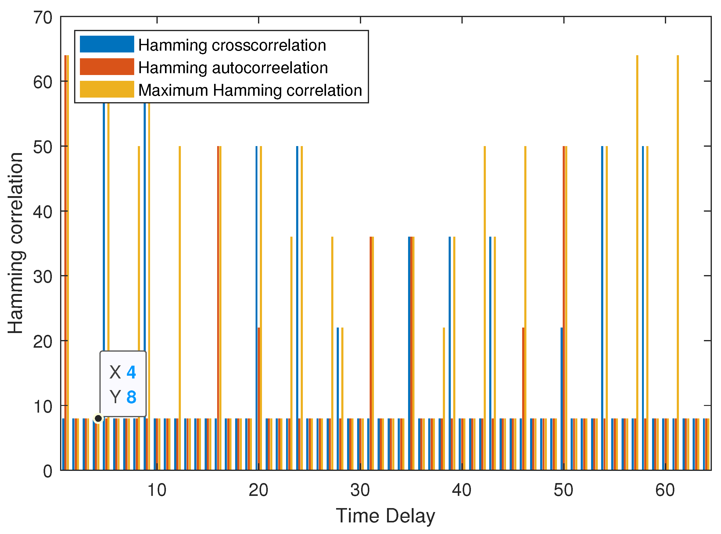
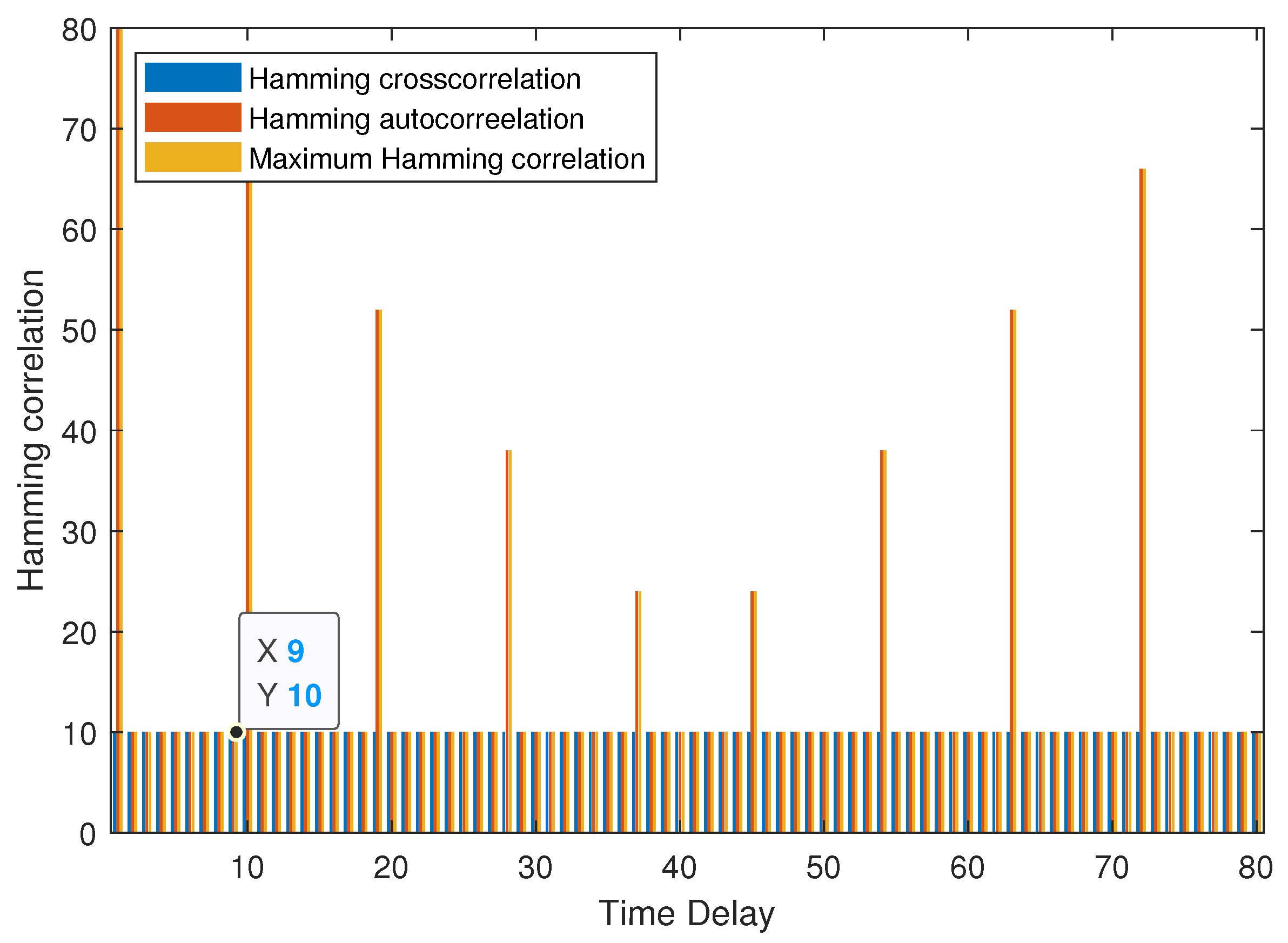
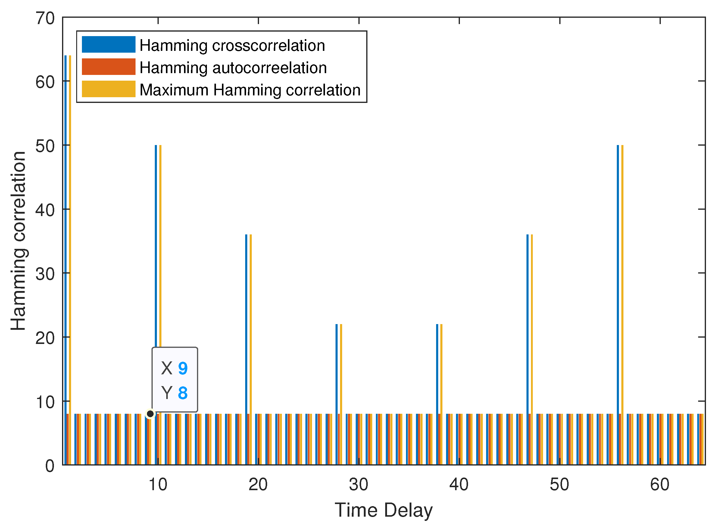
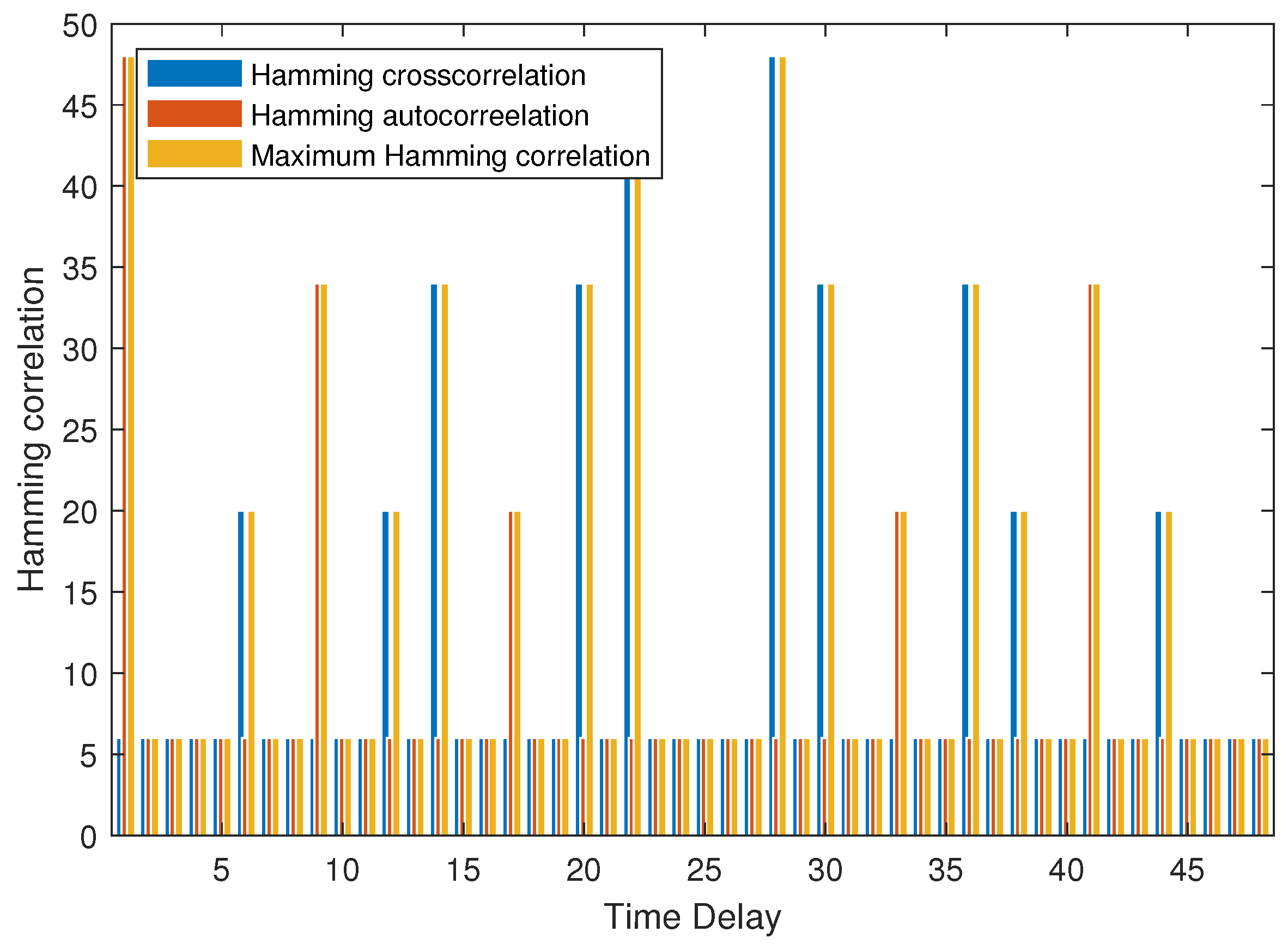
4. Optimal FHS Set with LHZ

In this section, the optimal LHZ FHS set with the new parameters is constructed based on different shift sequences through the interleaving technique [23,24].

Construction 1. 

Step 1: Select an optimal FHS set $\mathcal{A}$$(L,N,c,H_m\left(\mathcal{A}\right))$ that satisfies the Peng–Fan bound, $\mathcal{A}=\left\{a^i=\left(a_0^i,a_1^i,\dots ,a_{L-1}^i\right)\mid 0\le i<N\right\}$.

• Step 2: Let $T,u,k$ be three positive integers, $\theta$ is an integer, $T>2$, $uT=L$ and $k=u-1$. The shift sequence $\mathcal{E}=\left\{e_i^j\mid 0\le i<T,0\le j<k\right\}$. We have

  $$e_i^j=\left(e_0^j,e_1^j,\dots ,e_{T-1}^j\right)=(\theta \pm j,\theta +u\pm j,\dots ,\theta +(T-1)u\pm j).$$
• Step 3: Construct the LHZ FHS set $\mathcal{B}=\left\{b^p\mid 0\le p<kN\right\}$, $p=ik+j(0\le j<k,0\le i<N)$, where for each $0\le p<kN,$

  $$b^p=b^{ik+j}=I\left(L^{\theta \pm j}\left(a^i\right),L^{\theta +u\pm j}\left(a^i\right),\dots ,L^{\theta +(T-1)u\pm j}\left(a^i\right)\right)$$

Theorem 2. 

The LHZ FHS set $\mathcal{B}$$(TL,kN,c,T-1,T{H}_m\left(\mathcal{A}\right))$ constructed by Construction 1 is an optimal LHZ FHS set if T satisfies $T\lceil \frac{(NL-c)L}{(NL-1)c}\rceil =\lceil T\frac{\left(N\right(L-T)-c)L}{\left(N\right(L-T)-1)c}\rceil$. By permuting the sequences within a set of shift sequences, the resulting set of sequences is also an optimal LHZ FHS set.

Proof of Theorem 2. 

The shift sequence set is represented by a $kT$ matrix,

$$\begin{array}{cc}\hfill \mathcal{E}=& \left(\begin{array}{cccc}{e}_0^0& e_1^0& \dots & e_{T-1}^0\\ e_0^1& e_1^1& \dots & e_{T-1}^1\\ \dots & \dots & \dots & \dots \\ e_0^{k-1}& e_1^{k-1}& \dots & e_{T-1}^{k-1}\end{array}\right)\hfill \\ \hfill =& \left(\begin{array}{cccc}\theta & \theta +u& \dots & \theta +(T-1)u\\ \theta \pm 1& \theta \pm 1+u& \dots & \theta \pm 1+(T-1)u\\ \cdots & \cdots & \cdots & \cdots \\ \theta \pm (k-1)& \theta \pm (k-1)+u& \dots & \theta \pm (k-1)+(T-1)u\end{array}\right).\hfill \end{array}$$

The $e^j$ can be written as the following two cases.

Case 1:

$$\left\{\begin{array}{c}{e}_i^j=e_i^{j+s}-s,\\ e_i^j=e_{i+1}^{j+t}-u-t,\end{array}\right.$$

(3)

Case 2:

$$\left\{\begin{array}{c}{e}_i^j=e_i^{j+s}+s,\\ e_i^j=e_{i+1}^{j+t}-u+t,\end{array}\right.$$

(4)

where $0\le i+1\le T-1,0\le j+t,j+s\le k-1.$ From (3), we have

$$e_i^j=e_i^{j+s}-s=e_{i+1}^{j+t}-u-t.$$

(5)

From (5), we have

$$e_i^{j+s}=e_{i+1}^{j+t}-u-t+s.$$

(6)

We can obtain the relationship between the parameters of the rows and columns in the shift matrix from the above equation.

If any parameter meets the condition $s=u+t$, then $(s-t)T=L$. But the maximum value of $s-t$ is $k-1$. Therefore, the shift sequence $e_i^j$ are not identical to each other.

It can be learned from (5) that when $s=1$ and ${\tau }_2=0$, the value

$$\underset{e^{j_1},e^{j_2}\in \mathcal{E}}{min}\left\{\underset{0<t<T}{min}\left\{d_{t,{\tau }_2}^{e^{j_1},e^{j_2}}\right\}\right\}=1.$$

Therefore, from the Theorem 2, the LHZ $Z_h$ of $\mathcal{B}$ is $T-1$. The same analysis as above for (4), the LHZ $Z_h$ of $\mathcal{B}$ is $T-1$.

Concurrently, if the columns of the shift matrix are transformed, different representations of the shift matrix can be obtained. The following shift matrix is one of such representations.

$$\begin{array}{cc}\hfill \mathcal{E}=& \left(\begin{array}{cccc}{e}_v^0& e_{T-1}^0& \dots & e_1^0\\ e_v^1& e_{T-1}^1& \dots & e_1^1\\ \dots & \dots & \dots & \dots \\ e_v^{k-1}& e_{T-1}^{k-1}& \dots & e_1^{k-1}\end{array}\right)\hfill \\ \hfill =& \left(\begin{array}{cccc}\theta +vu& \theta +(T-1)u& \dots & \theta +u\\ \theta \pm 1+vu& \theta \pm 1+(T-1)u& \dots & \theta \pm 1+u\\ \cdots & \cdots & \cdots & \cdots \\ \theta \pm (k-1)+vu& \theta \pm (k-1)+(T-1)u& \dots & \theta \pm (k-1)+u\end{array}\right),\hfill \end{array}$$

where $1<v<T-1$. Based on the above proof, it can be shown that each element in a shift matrix is distinct and shift matrices do not collide with each other in rows and columns. Therefore, we have the LHZ $Z_h$ of $\mathcal{B}$ is $T-1$.

Moreover, we have

$$H_m\left(\mathcal{A}\right)=⌈\frac{(NL-c)L}{(NL-1)c}⌉.$$

According to Lemma 2, the MHC $H_m\left(\mathcal{B}\right)$$(TL,kN,c,T-1,H_m\left(\mathcal{B}\right))$ of FHS set $\mathcal{B}$ is

$$\begin{array}{cc}\hfill & H_m\left(\mathcal{B}\right)\ge T\frac{\left(kN\right(T-1)+kN-c)L}{\left(kN\right(T-1)+kN-1)c}=T\frac{(kNT-c)L}{(kNT-1)c}=T\frac{\left(NT\right(u-1)-c)L}{\left(NT\right(u-1)-1)c}\hfill \\ \hfill & =T\frac{\left(N\right(L-T)-c)L}{\left(N\right(L-T)-1)c}.\hfill \end{array}$$

For $T\lceil \frac{(NL-c)L}{(NL-1)c}\rceil =\lceil T\frac{\left(N\right(L-T)-c)L}{\left(N\right(L-T)-1)c}\rceil$, the MHC of $\mathcal{B}$ is the value that satisfies the equal sign of the Peng–Fan–Lee bound. In a word, the LHZ FHS set $\mathcal{B}$ is said to be the optimal. □

Example 1. 

Select an optimal (16, 3, 7, 2) FHS set $\mathcal{A}=\{a^0,a^1,a^2\}$, where

$$\begin{array}{cc}\hfill & a^0=\{1,0,1,6,2,4,5,6,6,0,6,1,5,3,2,1\},\hfill \\ \hfill & a^1=\{2,3,6,4,2,2,0,2,5,4,1,3,5,5,0,5\},\hfill \\ \hfill & a^2=\{6,3,3,0,3,4,6,5,1,4,4,0,4,3,1,2\}.\hfill \end{array}$$

One can obtain the shift sequences $\mathcal{E}=\{e^j=e_0^j,e_1^j,e_2^j,e_3^j\},0\le j<3$, such that $e^0=\{0,4,8,12\},e^1=\{15,3,7,11\},e^2=\{14,2,6,10\}$. It follows that

$$\mathcal{E}=\left(\begin{array}{cccc}{e}_0^0\hfill & e_1^0\hfill & e_2^0\hfill & e_3^0\hfill \\ e_0^1\hfill & e_1^1\hfill & e_2^1\hfill & e_3^1\hfill \\ e_0^2\hfill & e_1^2\hfill & e_2^2\hfill & e_3^2\hfill \end{array}\right)=\left(\begin{array}{cccc}0& 4& 8& 12\\ 15& 3& 7& 11\\ 14& 2& 6& 10\end{array}\right).$$

Construct the LHZ FHS set $\mathcal{B}=\{b^0,b^1,b^2,b^3,b^4,b^5,b^6,b^7,b^8\}$ by the Construction 1, where

$$\begin{array}{cc}\hfill & b^0=\{1,2,6,5,0,4,0,3,1,\cdots ,1,6,6,1\},b^1=\{1,6,6,1,1,2,6,5,0,\cdots ,2,1,5,6\},\hfill \\ \hfill & b^2=\{2,1,5,6,1,6,6,1,1,\cdots ,3,0,4,0\},b^3=\{2,2,5,5,3,2,4,5,6,\cdots ,5,4,2,3\},\hfill \\ \hfill & b^4=\{5,4,2,3,2,2,5,5,3,\cdots ,0,6,0,1\},b^5=\{0,6,0,1,5,4,2,3,2,\cdots ,5,3,2,4\},\hfill \\ \hfill & b^6=\{6,3,1,4,3,4,4,3,3,\cdots ,2,0,5,0\},b^7=\{2,0,5,0,6,3,1,4,3,\cdots ,1,3,6,4\},\hfill \\ \hfill & b^8=\{1,3,6,4,2,0,5,0,6,\cdots ,3,3,4,4\}.\hfill \end{array}$$

As shown in Figure 1, the MHC of set $\mathcal{B}$ is 8 when the $0<\tau \le 3$. It can be verified that $H_m\left(\mathcal{B}\right)=8$ for $\tau \le 3$, thus $\mathcal{B}$ is an optimal (64, 9, 7, 3, 8) LHZ FHS set.

Construction 2. 

Step 1: Select an optimal $(L,N,c,H_m\left(\mathcal{A}\right))$ FHS set $\mathcal{A}$ with respect to the Peng–Fan bound.

$$\mathcal{A}=\left\{a^j=\left(a_0^j,a_1^j,\dots ,a_{L-1}^j\right)\mid 0\le j<N\right\}.$$

Step 2: Select two integers $\theta ,T$ and a positive integer w, $T\ge 2$. Then, generate a shift sequence $\mathcal{E}=\{e_i\mid 0\le i<T\}$ as follows,

$$\mathcal{E}=\left(e_0,e_1,\dots ,e_{T-1}\right)=(\theta ,\theta +w,\dots ,\theta +(T-1)w).$$

Step 3: Construct a new set of FHS $\mathcal{B}=\left\{b^j=\left\{b^j\left(x\right)\mid 0\le x<TL\right\},0\le j<L\right\}$,

$$b^j=I\left(L^{\theta }\left(a^i\right),L^{\theta +w}\left(a^i\right),\dots ,L^{\theta +(T-1)w}\left(a^i\right)\right)$$

Theorem 3. 

The LHZ FHS set constructed by Construction 2 is an optimal LHZ FHS set if the parameters meet the following conditions. If $w<\frac{L+1}{2}$, T satisfies $T⌈\frac{(NL-c)L}{(NL-1)c}⌉=⌈\frac{T\left(N\right(Tw-1)-c)L}{\left(N\right(Tw-1)-1)c}⌉$ then $\mathcal{B}$$(TL,N,c,Tw-2,T{H}_m\left(\mathcal{A}\right))$ is an optimal LHZ FHS set. If $w>\frac{L+1}{2}$ and T satisfies $T⌈\frac{(NL-c)L}{(NL-1)c}⌉=⌈\frac{\left(NT\right(L-w)+N-c)TL}{\left(NT\right(L-w)+N-1)c}⌉$ then $\mathcal{B}$$(TL,N,c,T(L-w),T{H}_m\left(\mathcal{A}\right))$ is an optimal LHZ FHS set.

Proof of Theorem 3. 

We have

$$d_{t,{\tau }_2}^{(e,e)}=\left\{\begin{array}{c}{e}_t-e_{t+{\tau }_2},0\le t\le T-1+{\tau }_2\\ e_t-e_{t+{\tau }_2-T}-1,T-{\tau }_2\le t\le T-1\end{array}\right..$$

From the parameters of the shift sequence set in Construction 2, we have

$$\begin{array}{c}\hfill d_{t,{\tau }_2}^{(e,e)}=\left\{\begin{array}{c}-w{\tau }_2,0\le t\le T-1+{\tau }_2\\ w\left(T-{\tau }_2\right)-1,T-{\tau }_2\le t\le T-1\end{array}\right..\end{array}$$

Therefore, if $w<\frac{L+1}{2}$ and ${\tau }_2=T-1$, the minimum value of $d_{t,{\tau }_2}^{(e,e)}$ is $w-1$. Then,

$$Z_h=T(w-1)+{\tau }_2-1=Tw-2.$$

If $w>\frac{L+1}{2}$ and ${\tau }_2=1$, the minimum value of $d_{t,{\tau }_2}^{(e,e)}$ is $L-w$. Then,

$$Z_h=T(L-w).$$

Furthermore, we have

$$H_m\left(\mathcal{A}\right)=\frac{(NL-c)L}{(NL-1)c}.$$

According to Lemma 2, the MHC $H_m\left(\mathcal{B}\right)$ of FHS $\mathcal{B}$$(TL,N,c,H_m\left(\mathcal{B}\right))$ is

Case 1: when $w<\frac{L+1}{2}$,

$$\begin{array}{cc}\hfill & H_m\left(\mathcal{B}\right)\ge \frac{\left(NZ+N-c\right)L}{\left(NZ+N-1\right)c}=\frac{\left(N\right(Tw-2)+N-c)TL}{\left(N\right(Tw-2)+N-1)c}=\frac{\left(N\right(Tw-1)-c)TL}{\left(N\right(Tw-1)-1)c}.\hfill \end{array}$$

For

$$T⌈\frac{(NL-c)L}{(NL-1)c}⌉=⌈\frac{T\left(N\right(Tw-1)-c)L}{\left(N\right(Tw-1)-1)c}⌉,$$

the MHC of $\mathcal{B}$ is the value that satisfies the equal sign of the Peng–Fan–Lee bound.

Case 2: when $w>\frac{L+1}{2}$,

$$\begin{array}{cc}\hfill & H_m\left(\mathcal{B}\right)\ge \frac{\left(NZ+N-c\right)TL}{\left(NZ+N-1\right)c}=\frac{\left(NT\right(L-w)+N-c)TL}{\left(NT\right(L-w)+N-1)c}\hfill \end{array}$$

For

$$T⌈\frac{(NL-c)L}{(NL-1)c}⌉=⌈T\frac{\left(NT\right(L-w)+N-c)L}{\left(NT\right(L-w)+N-1)c}⌉,$$

the MHC of $\mathcal{B}$ is the value that satisfies the equal sign of the Peng–Fan–Lee bound.

Therefore, the LHZ FHS set $\mathcal{B}$ is said to be the optimal. □

Example 2. 

Select an optimal (16, 3, 7, 2) FHS set $\mathcal{A}=\{a^0,a^1,a^2\}$, where

$$\begin{array}{cc}\hfill & a^0=\{1,0,1,6,2,4,5,6,6,0,6,1,5,3,2,1\},\hfill \\ \hfill & a^1=\{2,3,6,4,2,2,0,2,5,4,1,3,5,5,0,5\},\hfill \\ \hfill & a^2=\{6,3,3,0,3,4,6,5,1,4,4,0,4,3,1,2\}.\hfill \end{array}$$

We set the parameters $\theta =1,w=2,T=5$. Then, the shift sequence is $\mathcal{E}=\{1,3,5,7,9\}$.

Construct the LHZ FHS set $\mathcal{B}=\{b^0,b^1,b^2\}$ where

$$\begin{array}{cc}\hfill & b^0=\{0,6,4,6,0,1,2,5,6,6,6,4,6,0,\cdots ,6,1,1,2,5,6\}\hfill \\ \hfill & b^1=\{3,4,2,2,4,6,2,0,5,1,4,2,2,4,\cdots ,2,2,6,2,0,5\}\hfill \\ \hfill & b^2=\{3,0,4,5,4,3,3,6,1,4,0,4,5,4,\cdots ,5,6,3,3,6,1\}\hfill \end{array}$$

As shown in Figure 2, the MHC of set $\mathcal{B}$ is 10 when the $\tau \le 8$. It can be verified that $⌈\frac{\left(NZ+N-c\right)L}{\left(NZ+N-1\right)c}⌉=10$, then $\mathcal{B}$ is an optimal (80, 3, 7, 8, 10) LHZ FHS set.

Example 3. 

Select an optimal (16, 7, 3, 2) FHS set $\mathcal{A}=\{a^0,a^1,a^2\}$, such that

$$\begin{array}{cc}\hfill & a^0=\{1,0,1,6,2,4,5,6,6,0,6,1,5,3,2,1\},\hfill \\ \hfill & a^1=\{2,3,6,4,2,2,0,2,5,4,1,3,5,5,0,5\},\hfill \\ \hfill & a^2=\{6,3,3,0,3,4,6,5,1,4,4,0,4,3,1,2\}.\hfill \end{array}$$

We set the parameters $\theta =1,w=14,T=4$, the shift sequence is $\mathcal{E}=\{1,15,13,11\}$.

Construct the LHZ FHS set $\mathcal{B}=\{b^0,b^1,b^2\}$ where

$$\begin{array}{cc}\hfill & b^0=\{0,1,3,1,1,1,2,5,6,0,1,3,2,1,1,\cdots ,1,0,1,2,5,6\},\hfill \\ \hfill & b^1=\{3,5,5,3,6,2,0,5,4,3,5,5,2,6,2,\cdots ,3,4,2,0,5,1\},\hfill \\ \hfill & b^2=\{3,2,3,0,3,6,1,4,0,3,2,3,3,3,6,\cdots ,0,4,6,1,4,4\}.\hfill \end{array}$$

As shown in Figure 3, the MHC of set $\mathcal{B}$ is 8 when the time delay $\tau \le 8$. It can be verified that $⌈\frac{\left(NZ+N-c\right)L}{\left(NZ+N-1\right)c}⌉=8$, then $\mathcal{B}$ is an optimal (64, 3, 7, 8, 8) LHZ FHS set.

Construction 3. 

Step 1: Select an optimal $(L,N,c,H_m\left(\mathcal{A}\right))$ FHS set $\mathcal{A}$ that satisfies the Peng–Fan bound, $\mathcal{A}=\left\{a^i=\left(a_0^i,a_i^i,\dots ,a_{L-1}^i\right),0\le i<N\right\}$.

• Step 2: Let T, u, k be three positive integers. w, $\theta$ are two integers, $T>2$, $w>1$ and $w=\theta +uT$. The shift sequence is $\mathcal{E}=\left\{e_i^j\mid 0\le i<T,0\le j<k\right\}$. We have

  $$\begin{array}{c}\hfill e^j=\left(e_0^j,e_1^j,\dots ,e_{T-1}^j\right)=(\theta +jw,\theta +u+jw,\dots ,\theta +(T-1)u+jw).\end{array}$$
• Step 3: Construct LHZ FHS set $\mathcal{B}=\left\{b^p\mid 0\le p<kN\right\}$, $p=ik+j(0\le i<N,0\le j<k)$, where for each $0\le p<kN,$

  $$b^p=I\left(L^{\theta +jw}\left(a^i\right),L^{\theta +u+jw}\left(a^i\right),\dots ,L^{\theta +(T-1)u+jw}\left(a^i\right)\right).$$

Theorem 4. 

The LHZ FHS set $\mathcal{B}$ constructed by Construction 3 is an optimal $\mathcal{B}$$(TL,kN,c,2T-2,$$T{H}_m\left(\mathcal{A}\right))$ LHZ FHS set if parameter meets $k(2T-1)\le L$, $u(kT-1)=L-1$ and $T\lceil \frac{(NL-c)L}{(NL-1)c}\rceil =⌈T\frac{\left(kN\right(2T-1)-c)L}{\left(kN\right(2T-1)-1)c}⌉$.

Proof of Theorem 4. 

The shift sequence set is represented by a $kT$ matrix,

$$\begin{array}{cc}\hfill \mathcal{E}=& \left(\begin{array}{cccc}{e}_0^0& e_1^0& \dots & e_{T-1}^0\\ e_0^1& e_1^1& \dots & e_{T-1}^1\\ \dots & \dots & \dots & \dots \\ e_0^{k-1}& e_1^{k-1}& \dots & e_{T-1}^{k-1}\end{array}\right)\hfill \\ \hfill =& \left(\begin{array}{cccc}\theta & \theta +u& \dots & \theta +(T-1)u\\ \theta +w& \theta +u+w& \dots & \theta +(T-1)u+w\\ \dots & \dots & \dots & \dots \\ \theta +(k-1)w& \theta +u+(k-1)w& \dots & \theta +(T-1)u+(k-1)w\end{array}\right)\hfill \end{array}$$

The $e^j$ can be written as

$$\begin{array}{c}\left\{\begin{array}{c}{e}_i^j=e_{i+s}^{j-s}-s(u-w),\\ e_i^j=e_i^{j\pm 1}\pm w,\end{array}0<i+s,j-s<T\right.\end{array}$$

(7)

From (7), we have

$$e_i^j=e_{i+s}^{j-s}-s(u-w)=e_i^{j\pm 1}\pm w.$$

(8)

From (8), we have

$$e_{i+s}^{j-s}=e_i^{j\pm 1}\pm w+s(u-w).$$

(9)

For $u(kT-1)=L-1$, then $\theta -(\theta +(T-1)u+(k-1\left)w\right)$ (mod L) = 1. From (8) and (9), $\pm w$ (mod L) ≥ 1, $sw-su$ (mod L) $\ge 1$ for $T>2$ and $w=\theta +uT$. Thus,

$$\underset{e^{j_1},e^{j_2}\in E}{min}\left\{\underset{0<i<T}{min}\left\{d_{t,{\tau }_2}^{e^{j_1},e^{j_2}}\right\}\right\}=1.$$

At this time, the delay time ${\tau }_2$ is $T-1$, then

$$Z_h=\left\{T{d}_{t,\tau }^{(e^{j_1},e^{j_2})}+{\tau }_2\right\}-1=2T-2.$$

Besides, we have

$$H_m\left(\mathcal{A}\right)=\frac{(NL-c)L}{(NL-1)c},$$

According to Lemma 2, the MHC $H_m\left(\mathcal{B}\right)$$(TL,kN,c,H_m\left(\mathcal{B}\right),2T-2)$ of LHZ FHS set $\mathcal{B}$ is

$$\begin{array}{cc}\hfill & H_m\left(\mathcal{B}\right)\ge \frac{\left(kN\right(2T-2)+kN-c)TL}{\left(kN\right(2T-2)+kN-1)c}=T\frac{\left(kN\right(2T-1)-c)L}{\left(kN\right(2T-1)-1)c}.\hfill \end{array}$$

For

$$T⌈\frac{(NL-c)L}{(NL-1)c}⌉=⌈T\frac{\left(kN\right(2T-1)-c)L}{\left(kN\right(2T-1)-1)c}⌉,$$

the MHC of $\mathcal{B}$ is the value that satisfies the equal sign of Peng-Fan-Lee bound. All in all, the LHZ FHS set $\mathcal{B}$ is said to be the optimal. □

Example 4. 

Select an optimal (16, 3, 7, 2) FHS set $\mathcal{A}=\{a^0,a^1,a^2\}$, where

$$\begin{array}{cc}\hfill & a^0=\{1,0,1,6,2,4,5,6,6,0,6,1,5,3,2,1\},\hfill \\ \hfill & a^1=\{2,3,6,4,2,2,0,2,5,4,1,3,5,5,0,5\},\hfill \\ \hfill & a^2=\{6,3,3,0,3,4,6,5,1,4,4,0,4,3,1,2\}.\hfill \end{array}$$

We set the parameters $\theta =0,T=3,k=2,w=9,u=3$, the shift sequences $e^0=\{0,3,6\}$, $e^1=\{9,12,15\}$. It follows that

$$\mathcal{E}=\left(\begin{array}{ccc}{e}_0^0\hfill & e_1^0\hfill & e_2^0\hfill \\ e_0^1\hfill & e_1^1\hfill & e_2^1\hfill \end{array}\right)=\left(\begin{array}{ccc}0& 3& 6\\ 9& 12& 15\end{array}\right).$$

We construct the LHZ FHS set $\mathcal{B}=\{b^0,b^1,b^2,b^3,b^4,b^5\}$ where

$$\begin{array}{cc}\hfill & b^0=\{1,6,5,0,2,6,1,4,6,6,5,0,\cdots ,2,0,2,1,1,4\},\hfill \\ \hfill & b^1=\{0,5,1,6,3,1,1,2,0,5,1,1,\cdots ,6,6,3,6,1,2\},\hfill \\ \hfill & b^2=\{2,4,0,3,2,2,6,2,5,4,0,4,\cdots ,0,3,2,5,6,2\},\hfill \\ \hfill & b^3=\{4,5,5,1,5,2,3,0,3,5,5,6,\cdots ,2,1,5,5,3,0\},\hfill \\ \hfill & b^4=\{6,0,6,3,3,5,3,4,1,0,6,4,\cdots ,1,3,3,2,3,4\},\hfill \\ \hfill & b^5=\{4,4,2,4,3,6,0,1,3,4,2,3,\cdots ,5,4,3,1,0,1\}.\hfill \end{array}$$

As shown in Figure 4, the MHC of set $\mathcal{B}$ is 6 when the $\tau \le 4$. It can be verified that $⌈\frac{\left(NZ+N-c\right)L}{\left(NZ+N-1\right)c}⌉=6$, then $\mathcal{B}$ is an optimal (48, 6, 7, 4, 6) LHZ FHS set.

5. Conclusions

In this paper, we propose three new methods for the construction of the optimal LHZ FHS set and prove some sufficient conditions that they need to satisfy. As a comparison, we list the parameters of the existing optimal LHZ FHS sets and the optimal LHZ FHS sets constructed in this paper in

Table 1. Comparison of parameters for LHZ FHS sets with optimal Hamming correlation.

Parameters $(\mathit{L},\mathit{N},\mathit{c},{\mathit{Z}}_{\mathit{h}},{\mathit{H}}_{\mathit{m}}\left(\mathcal{Q}\right))$	Constraints	Ref.
$(s(q^n-1),M,q,w-1,$ $s(q^{n-1}-1))$	$q^n-1=wm,gcd(s,q^n-1)=1.$	[6]
$(s(p^n-1),e,e+1,w-1,sf)$	$gcd(s,p^n-1)=1,w=\frac{p^n-1}{m},m|(p^n-1),$ $1\le m<f$, $e+1>sf$, $sf{e}^{2}m<(f{e}^2-m)(e+1-sf).$	[13]
$(sN,mM,v,w-1,s\lambda )$	$m=\lceil \frac{N}{w}\rceil$, $gcd(s,N)=1,s=aw+1$, $a\ge 1$, $s<mN$.	[9]
$(MN,m,v,wM-1,M\lambda )$	$m=\lceil \frac{N}{w}\rceil$.	[8]
$(MN,m,v,M-2,M\lambda )$	$m=\lceil \frac{N}{w}\rceil$, $w>2M$.	[16]
$(TL,kN,c,T-1,T{H}_m\left(\mathcal{A}\right))$	$uT=L$, $k=u-1$, $T⌈\frac{(NL-c)L}{(NL-1)c}⌉=⌈T\frac{\left(N\right(L-T)-c)L}{\left(N\right(L-T)-1)c}⌉$	Construction 1
$(TL,N,c,Tw-2,T{H}_m\left(\mathcal{A}\right))$	$w<\frac{L+1}{2}$, $T⌈\frac{(NL-c)L}{(NL-1)c}⌉=⌈\frac{T\left(N\right(Tw-1)-c)L}{\left(N\right(Tw-1)-1)c}⌉$	Construction 2
$(TL,N,c,T(L-w),T{H}_m\left(\mathcal{A}\right))$	$w>\frac{L+1}{2}$, $T⌈\frac{(NL-c)L}{(NL-1)c}⌉=⌈\frac{\left(NT\right(L-w)+N-c)TL}{\left(NT\right(L-w)+N-1)c}⌉$	Construction 2
$(TL,kN,c,2T-2,T{H}_m\left(\mathcal{A}\right))$	$k(2T-1)\le L$, $u(kT-1)=L-1$, $T⌈\frac{(NL-c)L}{(NL-1)c}⌉=⌈T\frac{\left(kN\right(2T-1)-c)L}{\left(kN\right(2T-1)-1)c}⌉$	Construction 3

. As a result, our constructed sequences are more flexible and can be used to eliminate MI in QS FHMA systems. Future work can explore the application of FHSs in more scenarios, such as image processing, data encryption, mobile communication, security and privacy. Overall, exploring the application of FHSs in various scenarios can lead to new innovations and improvements in different areas of wireless communication.

References

1. Golomb, S.W.; Gong, G. Signal Design for Good Correlation: For Wireless Communication, Cryptography, and Radar; Cambridge University Press: New York, NY, USA, 2005. [Google Scholar]
2. Fan, P.; Darnell, M. Sequence Design for Communications Applications; Research Studies Press: London, UK, 1996; pp. 271–350. [Google Scholar]
3. Li, Z.; Chang, Y.; Jin, L.J. A novel family of frequency hopping sequences for multi-hop Bluetooth networks. IEEE Trans. Consum. Electron. 2003, 49, 1084–1089. [Google Scholar]
4. Peng, D.; Fan, P. Lower bounds on the Hamming auto- and cross correlations of frequency-hopping sequences. IEEE Trans. Inf. Theory 2004, 50, 2149–2154. [Google Scholar] [CrossRef]
5. Peng, D.; Fan, P.; Lee, M.H. Lower bounds on the periodic Hamming correlations of frequency hopping sequences with low hit zone. Sci. China Ser. F Inf. Sci. 2006, 49, 208–218. [Google Scholar] [CrossRef]
6. Ma, W.; Sun, S. New designs of frequency hopping sequences with low hit zone. Des. Codes Cryptogr. 2011, 60, 145–153. [Google Scholar] [CrossRef]
7. Chung, J.H.; Han, Y.; Yang, K. New Classes of Optimal Frequency-Hopping Sequences by Interleaving Techniques. IEEE Trans. Inf. Theory 2009, 55, 5783–5791. [Google Scholar] [CrossRef]
8. Niu, X.; Peng, D.; Zhou, Z. Frequency/time hopping sequence sets with optimal partial Hamming correlation properties. Sci. China Ser. F Inf. Sci. 2012, 55, 2207–2215. [Google Scholar] [CrossRef]
9. Niu, X.; Peng, D.; Zhou, Z. New Classes of Optimal Low Hit Zone Frequency Hopping Sequences with New Parameters. IEICE Trans. Fundam. 2014, 95, 1835–1842. [Google Scholar] [CrossRef] [Green Version]
10. Cai, H.; Yang, Y.; Zhou, Z.; Tang, X. Strictly Optimal Frequency-Hopping Sequence Sets With Optimal Family Sizes. IEEE Trans. Inf. Theory 2016, 62, 1087–1093. [Google Scholar]
11. Cai, H.; Zhou, Z.C.; Yang, Y.; Tang, X.H. A New Construction of Frequency-Hopping Sequences With Optimal Partial Hamming Correlation. IEEE Trans. Inf. Theory 2014, 60, 5782–5790. [Google Scholar]
12. Han, H.; Peng, D.; Parampalli, U. New sets of optimal low-hit-zone frequency-hopping sequences based on m-sequences. Cryptogr. Commun. 2017, 9, 511–522. [Google Scholar] [CrossRef]
13. Wang, C.; Peng, D.; Zhou, L. New Constructions of Optimal Frequency-Hopping Sequence Sets with Low-Hit-Zone. Int. J. Found. Comput. Sci. 2016, 27, 53–66. [Google Scholar] [CrossRef]
14. Zhou, L.; Peng, D.; Liang, H.; Wang, C.Y.; Ma, Z. Constructions of optimal low-hit-zone frequency hopping sequence sets. Des. Codes Cryptogr.. 2017, 85, 219–232. [Google Scholar] [CrossRef]
15. Zhou, L.; Peng, D.; Liang, H.; Wang, C.; Han, H. Generalized methods to construct low-hit-zone frequency-hopping sequence sets and optimal constructions. Cryptogr. Commun. 2017, 9, 707–728. [Google Scholar] [CrossRef]
16. Ling, L.; Niu, X.; Zeng, B.; Liu, X. New classes of optimal low hit zone frequency hopping sequence set with large family size. IEICE Trans. Fundam. Electron. Commun. Comput. Sci. 2018, 101, 2213–2216. [Google Scholar] [CrossRef]
17. Niu, X.; Han, L.; Liu, X. New Extension Interleaved Constructions of Optimal Frequency Hopping Sequence Sets With Low Hit Zone. IEEE Access 2019, 7, 73870–73879. [Google Scholar] [CrossRef]
18. Niu, X.; Xing, C. New Extension Constructions of Optimal Frequency-Hopping Sequence Sets. IEEE Trans. Inf. Theory 2019, 56, 5846–5855. [Google Scholar] [CrossRef] [Green Version]
19. Han, H.; Zhou, L.; Liu, X. New Construction for Low Hit Zone Frequency Hopping Sequence Sets with Optimal Partial Hamming Correlation. In Proceedings of the 2019 Ninth International Workshop on Signal Design and its Applications in Communications (IWSDA), Dongguan, China, 20–24 October 2019; pp. 1–5. [Google Scholar]
20. Niu, X.; Xing, C.; Yuan, C. Asymptotic Gilbert–Varshamov Bound on Frequency Hopping Sequences. IEEE Trans. Inf. Theory 2020, 66, 1213–1218. [Google Scholar] [CrossRef] [Green Version]
21. Niu, X.; Xing, C.; Liu, Y.; Zhou, L. A Construction of Optimal Frequency Hopping Sequence Set via Combination of Multiplicative and Additive Groups of Finite Fields. IEEE Trans. Inf. Theory 2020, 66, 5310–5315. [Google Scholar] [CrossRef] [Green Version]
22. Zhou, L.; Liu, X.; Han, H.; Wang, C. Classes of optimal low-hit-zone frequency-hopping sequence sets with new parameters. Cryptogr. Commun. 2022, 14, 291–306. [Google Scholar] [CrossRef]
23. Gong, G. Theory and applications of q-ary interleaved sequences. IEEE Trans. Inf. Theory 1995, 41, 400–411. [Google Scholar] [CrossRef]
24. Gong, G. New designs for signal sets with low cross correlation, balance property, and large linear span: GF(p) case. IEEE Trans. Inf. Theory 2002, 48, 2847–2867. [Google Scholar] [CrossRef]
Figure 1. MHC of B in Example 1.
Entropy 25 01044 g001
Figure 2. MHC of B in Example 2.
Entropy 25 01044 g002
Figure 3. MHC of B in Example 3.
Entropy 25 01044 g003
Figure 4. MHC of B in Example 4.
Entropy 25 01044 g004