
Optimal Shortcuts to Adiabatic Control by Lagrange Mechanics

International Center of Quantum Artificial Intelligence for Science and Technology (QuArtist), Department of Physics, Shanghai University, Shanghai 200444, China
*
Author to whom correspondence should be addressed.
Entropy 2023, 25(5), 719; https://doi.org/10.3390/e25050719
Submission received: 1 February 2023
/
Revised: 3 April 2023
/
Accepted: 8 April 2023
/
Published: 26 April 2023
(This article belongs to the Special Issue Quantum Control and Quantum Computing)
Abstract
:We combined an inverse engineering technique based on Lagrange mechanics and optimal control theory to design an optimal trajectory that can transport a cartpole in a fast and stable way. For classical control, we used the relative displacement between the ball and the trolley as the controller to study the anharmonic effect of the cartpole. Under this constraint, we used the time minimization principle in optimal control theory to find the optimal trajectory, and the solution of time minimization is the bang-bang form, which ensures that the pendulum is in a vertical upward position at the initial and the final moments and oscillates in a small angle range.
1. Introduction
In the past few decades, with the development of experimental technology, the unstable control of nonlinear unstable systems [1,2,3,4,5] by a moving controller has attracted more and more attention. As far as we know, a sufficiently slow adiabatic process is a very simple way to achieve the ideal transfer, i.e., without excitations or losses [6,7,8,9]. However, a sufficiently slow process is problematic, firstly a sufficiently slow process, is impractically long and, secondly, over a long period of time, the ideal dynamics may be subject to the accumulation of random and/or uncontrollable perturbations that can undermine the expected results. In some experiments and theories, it is necessary to speed up this transport process but also to ensure that there is no excitation or loss at the initial and final moments [10,11,12,13,14,15,16,17]. To solve these problems, “Shortcuts To Adiabaticity” (STA) technology was proposed decades ago [18]. It achieves the same results as the adiabatic process in a short time [19]. At present, STA technology has been successfully applied to atoms, molecules, optical physics, solid state physics, chemistry, engineering, quantum systems, and classical systems [12,20,21,22,23,24,25]. With the development of STA technology, the STA technique includes many different schemes, such as the quantum invariant-based inverse control method [26,27,28,29], the reverse thermal transfer compensation method [30,31,32], the no-jump quantum drive method [33,34,35], etc. These methods have been validated in a number of experiments.
Cartpole is a typical multivariate, higher-order, nonlinear, strongly coupled, naturally unstable system. The stable control of the cartpole system is a typical problem in control theory. Here, we used the inverse engineering method, based on Lagrange mechanics, for a fast but stable control of the cartpole. By fixing the boundary conditions at the initial and final times, we aimed to find the trajectories that meet the boundary conditions [19,36] but that also achieves transition-free evolution ideally in a shorter time. Later, this approach can be complemented by optimal control theory [37,38], where we used the time minimization criterion in the Pontryagin maximization principle. Pontryagin’s maximum (or minimum) principle [39] is used in optimal control theory to find the best possible control for taking a dynamical system from one state to another, especially in the presence of constraints for the state or input controls. It was formulated in 1956 by the Russian mathematician Lev Semenovich Pontryagin and his students. The main thing is to find a controller so that the control Hamiltonian of the system reaches the maximum (or minimum) and then determines the optimal trajectory of the system. In this article, we used the relative displacement of the ball and the trolley horizontally as a controller, and then used the principle to find the optimal trajectory.
2. Physical Model
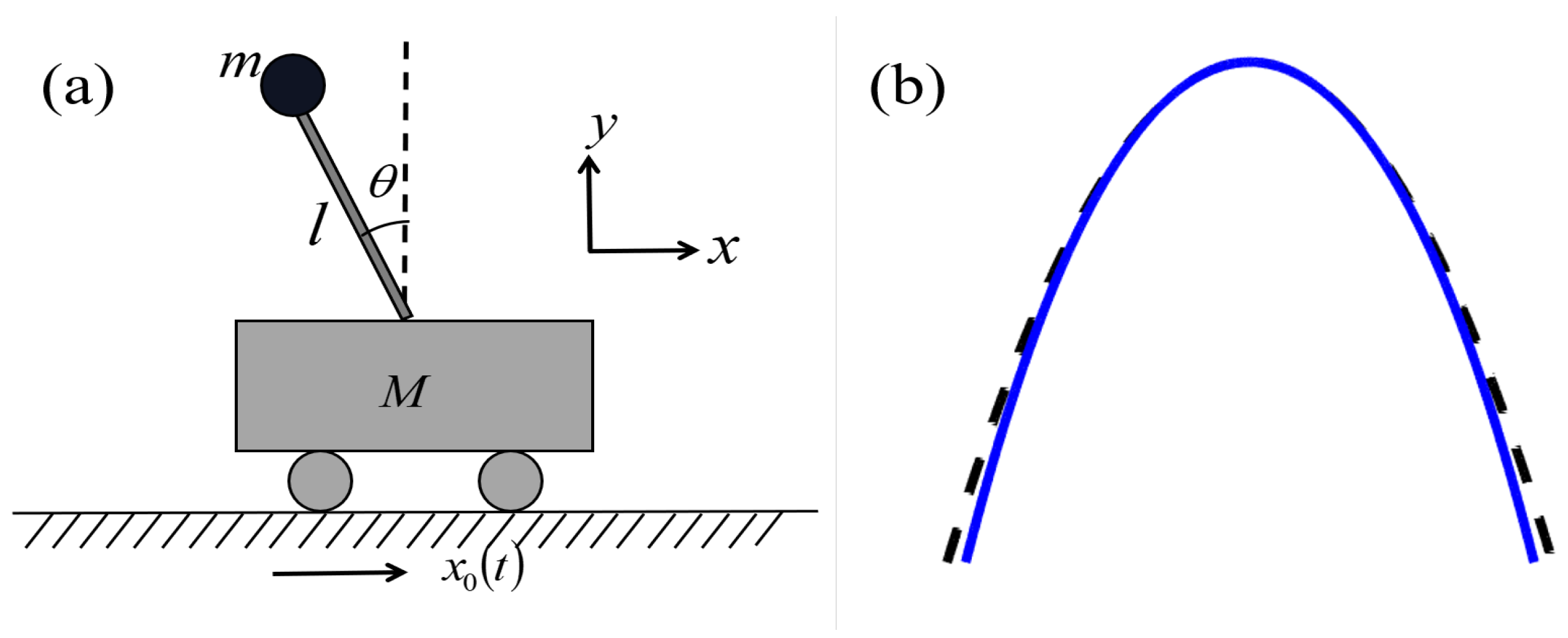
Here, we studied an ideal straight type cartpole system model; its schematic diagram and related parameters are shown in Figure 1. The trolley moves from and , swinging the pole as far as possible in a vertically upward position at the initial and final moments. Never a perfect harmonic in actual transmission, similar to the transport potential of approximate optical tweezers, the quartic anharmonic plays a very important role, as shown in Figure 1b. We aimed to combine the inverse engineering method [26,27,28,29] with the optimal control theory in the Pontryagin maximization principle [37,38]. By setting boundary conditions to suppress the final excitation, we used the relative distance between the ball and the trolley as a controller throughout the process, to achieve the time minimization.
The physical model and related parameters are shown in Figure 1, where M indicates the mass of the trolley, l is the length of the non-elongated rod, m is the mass of the ball, is the angle between the pole and the vertical direction, represents the position of the trolley over time, and x represents the position of the ball. We assumed that the model is an ideal model by setting the following conditions: (i) the quality and friction of the rod can be ignored; (ii) point masses; (iii) constant rod length l; (iv) the trolley position is treated as a control parameter rather than a dynamical variable.
3. Hamiltonian of the System and Inverse Engineering
The solution of the cartpole system can be solved by Lagrange mechanics. According to the parameters provided in Figure 1, the Cartesian coordinate of mass in a rest frame are given by:
where represents the position of the trolley. The kinetic energy and potential energy of the system can be expressed as follows:
where the dots represent time derivatives. It can be obtained by substituting Equation (1) into Equation (2),
Thus, the Lagrangian of the system can be written as:
Based on the Euler–Lagrange equation , we can obtain the corresponding dynamics equation as follows:
In order to reverse engineer the trajectory of the trolley, we need to calculate the Hamiltonian of the system, according to , where is the momentum with as the generalized coordinate. So, we need the conjugate momentum of ,
Thus, the Hamiltonian can be obtained from the Lagrangian:
Using the canonical transformation approach, change the system from to q as the coordinate, and the Hamiltonian is rewritten as (please refer to Appendix A for details):
where is the natural frequency of the pendulum, p represents the momentum with q as the generalized coordinate, . According to the canonical transformation [40], we can obtain:
from which the dynamic equation of the system becomes
This can be written as:
To fix the distance, we assumed that the trolley is transported from to . We can set suitable boundary conditions for according to our expectations, and based on these boundary conditions the trolley trajectory can be inverse engineered [26,27,28,29] to see how the position of the mass changes over time. We imposed the conditions as follows:
In general, there are different options from which to choose the trajectories fulfilling the boundary conditions. For instance, one can choose the polynomial ansatz to interpolate the function. In the following section, we would like to complement it with time-optimal control for this problem.
4. Optimal Control for Time Minimization
In this section, we try to find the time minimization by using the Pontryagin maximum principle [37,38]. To be consistent, we set new notations for the Equation (11) of motion of the system:
such that (where is the controller, representing the relative displacement of the ball to the trolley in the horizontal direction; x is the dynamic variable, representing the position of the ball)
For this system, the boundary conditions for , and can be given by Equations (11) and (12), and is required to satisfy at and . From the optimal control theory, one can find for a fixed bound and minimize the cost function J. The Pontryagin maximum principle finally provides the necessary conditions for optimal control [37,38].
For the relative displacement between the ball and the trolley, we utilized optimal control theory to find the time-optimal trajectory [38], so we defined the cost function as: . In this manner, we defined the control Hamiltonian as:
For almost all , the function attains its maximum at and , where c is constant, and . According to the cost function, the control Hamiltonian can be written as:
from which the canonical equations are
Accordingly, we can obtain the following costate equations by way of Equation (18):
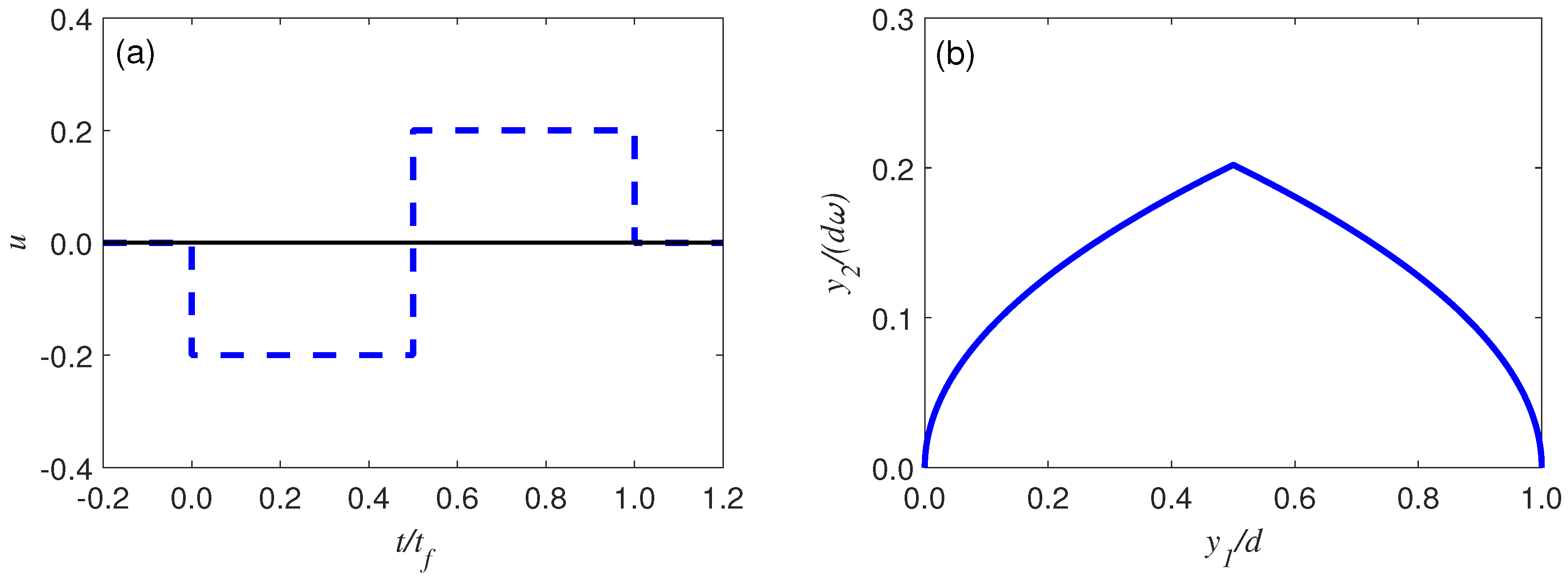
We can easily get and , where , are constant. In order to maximize the control of the Hamiltonian, we can obtain the optimal as a form of bang-bang control,
as shown in Figure 2, with only one intermediate switching time at . Since the controller is in the form of a switch, the trajectory of the trolley changes abruptly at . By substituting into Equation (11) and combining the boundary conditions in Equation (12), we eventually obtain the trajectory of ,
According to , the trajectory of the trolley can be represented as:
Solving the system of Equations (14) and (15), we find the switching time and final time as follows:
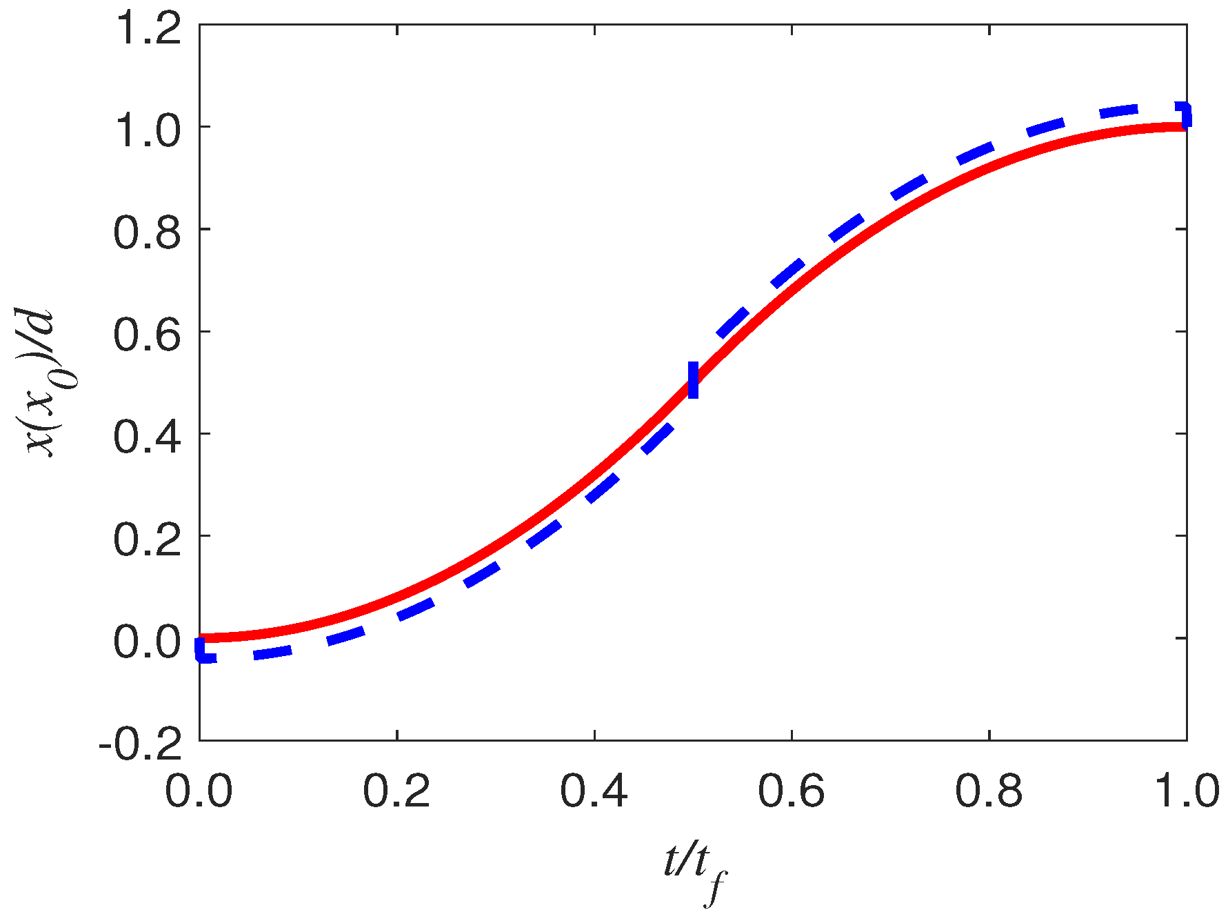
Again, the trajectory of the trolley and the trajectory of the swing ball are shown in Figure 3. Through the above control, the ball can be oscillated in a small angle range.
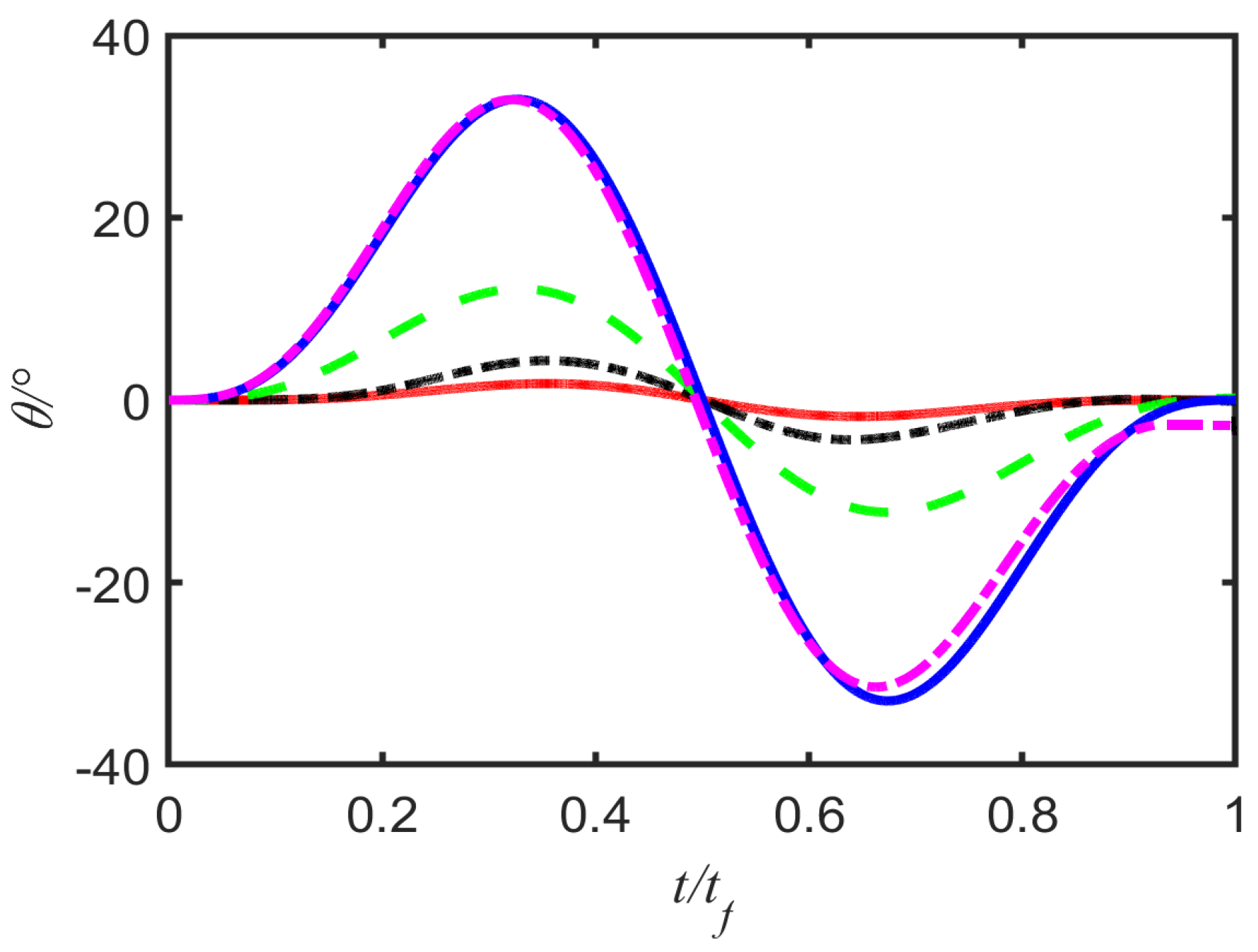
After finding the optimal trajectory, we brought it into the exact Equation (5) and approximate dynamic equations. Clearly, short times imply larger transient angles, as shown in Figure 4. In addition, for the long time, we can see that there is basically no big difference in the change of angle over time, but the difference is noticeable only for the smaller time, . The main reason is that if we ignore the higher-order terms, the approximation deviates from the reality. At the same time, because the is the relative displacement between the ball and the trolley, the maximum value of which is the length of the pendulum, when the has a fixed value, the will have a lower bound. In other words, when reaches a certain value, the transmission time of the system is relatively small, the speed is relatively large, and the system may break down so that the control is not very good. According to the analysis of physical meaning, when , in this case, the pendulum is in a “lying flat” state, that is, in horizontal direction, the system basically breaks down completely. In short, we can determine whether the system breaks down based on the change in relative displacement with .
5. Conclusions
In conclusion, we applied reverse engineering based on Lagrange mechanics and time minimization in the Pontriagin maximization principle for the fast but stable control of nonlinear unstable systems, e.g., the cartpole. In such control, we took an anharmonic effect and analyzed the stability of control. By fixing the relative displacement between the position of the ball and the trolley as constraints, we applied optimal control theory to design a time-optimal trajectory, as compared to the case of harmonic approximation. In the future, we will work out the classical control of the inverted double pendulum, and compare it with the control of the cartpole. Of course, the machine learning, fed by the results of STA, can be an interesting area for exploration as well.
Author Contributions
Formal analysis, L.M. and Q.K.; investigation, L.M. and Q.K.; methodology, Q.K.; writing—original draft preparation, L.M.; writing—review and editing, L.M. and Q.K.; supervision, Q.K. All authors have read and agreed to the published version of the manuscript.
Funding
This research was funded by the National Natural Science Foundation of China (Grant No. 12075145), STCSM (Grant No. 2019SHZDZX01-ZX04).
Institutional Review Board Statement
Not applicable.
Data Availability Statement
Not applicable.
Acknowledgments
We acknowledge the fruitful discussion with Yongcheng Ding.
Conflicts of Interest
The authors declare no conflict of interest.
Appendix A
The specific derivation of Equation (8) for the system is as follows: Start with Equation (4), according to , we can get:
We look for a canonical transformation to variables such that the new coordinate is the horizontal deviation from the suspension point . This transformation is achieved with the (time-dependent) generating function . generates the desired change of coordinate since:
The inertial effects is 0, so the Hamiltonian in the new variables is:
The last term introduces a linear-in-momentum term. To get rid of this term, we make a momentum shift by a second canonical transformation using the generating function,
The transformation equations to the new canonical variables are:
Including the inertial effects
the transformed Hamiltonian in the q and p variables is given by:
At the small angle approximation, , the Equation (A9) can be written as:
where is the natural frequency of the pendulum. Usually, the term can be ignored for second-order terms, but not for quartic terms. Here, we can not perform another canonical transformation to cancel this term, so we have to compromise by ignoring it in the next calculation, keeping other feasible high-order terms, and calculate the the controller. By numerical simulations of dynamics without any approximation, even though the term is neglected, the controller still has a satisfying performance. Somehow, we may conclude that, the effect of such term is not that significant.
References
- Fradkov, A.L. Swinging control of nonlinear oscillations. Int. J. Control 1996, 64, 1189–1202. [Google Scholar] [CrossRef]
- Chidambaram, M.; Jyothi, S.N. Control of Non-linear Unstable systems with Input Multiplicity. Indian Chem. Eng. 2001, 43, 99–100. [Google Scholar] [CrossRef]
- Kosmatopoulos, E.B. Control of Unknown Nonlinear Systems with Efficient Transient Performance Using Concurrent Exploitation and Exploration. IEEE Trans. Neural Netw. 2010, 21, 1245–1261. [Google Scholar] [CrossRef] [PubMed]
- Gorban, A.N.; Tyukin, I.Y.; Nijmeijer, H. Further Results on Lyapunov-Like Conditions of Forward Invariance and Boundedness for a Class of Unstable Systems. arXiv 2014, arXiv:2014.7039621. [Google Scholar]
- Wang, Q.D.; Jing, Y.W.; Zhang, S.Y. Global Adaptive Output Tracking Control of a Class of Nonlinear Systems. J. Northeast. Univ. 2004, 25, 817–820. [Google Scholar] [CrossRef]
- Greiner, M.; Bloch, I.; Hänsch, T.W.; Esslinger, T. Magnetic transport of trapped cold atoms over a large distance. Phys. Rev. A 2001, 63, 031401(R). [Google Scholar] [CrossRef]
- Schmid, S.; Thalhammer, G.; Winkler, K.; Lang, F.; Denschlag, J.H. Long distance transport of ultracold atoms using a 1D optical lattice. New J. Phys. 2006, 8, 159. [Google Scholar] [CrossRef]
- Dickinson, A.G.; Denker, J.S. Adiabatic dynamic logic. IEEE J. Solid-State Circuits 1995, 30, 311–315. [Google Scholar] [CrossRef]
- Gustavson, T.L.; Chikkatur, A.P.; Leanhardt, A.E.; Görlitz, A.; Gupta, S.; Pritchard, D.E.; Ketterle, W. Transport of Bose-Einstein condensates with optical tweezers. Am. Phys. Soc. 2001, 88, 020401. [Google Scholar] [CrossRef]
- Couvert, A.; Kawalec, T.; Reinaudi, G.; Guéry-Odelin, D. Optimal transport of ultracold atoms in the non-adiabatic regime. Europhys. Lett. 2008, 83, 13001. [Google Scholar] [CrossRef]
- Hauck, S.H.; Stojanovic, V.M. Coherent atom transport via enhanced shortcuts to adiabaticity: Double-well optical lattice. Phys. Rev. Appl. 2021, 18, 014016. [Google Scholar] [CrossRef]
- González-Resines, S.; Guéry-Odelin, D.; Tobalina, A.; Lizuain, I.; Torrontegui, E.; Muga, J. Invariant-based inverse engineering of crane control parameters. Phys. Rev. Appl. 2017, 8, 054008. [Google Scholar] [CrossRef]
- Hao, S.-Y.; Chen, Y.; Kang, Y.-E. Constructing shortcuts to the adiabatic passage for implementation of nongeomeric phase gates in a two-atom system. Laser Phys. Lett. 2021, 18, 10. [Google Scholar] [CrossRef]
- Klostermann, T.; Cabrera, C.R.; von Raven, H.; Wienand, J.F.; Schweizer, C.; Bloch, I.; Aidelsburger, M. Fast long-distance transport of cold cesium atoms. Phys. Rev. A 2021, 105, 4. [Google Scholar] [CrossRef]
- Chen, X.; Torrontegui, E.; Stefanatos, D.; Li, J.S.; Muga, J.G. Optimal trajectories for efficient atomic transport without final excitation. Phys. Rev. A 2011, 84, 043415. [Google Scholar] [CrossRef]
- Nakamura, K.; Matrasulov, J.; Izumida, Y. Fast-forward approach to stochastic heat engine. Phys. Rev. E 2020, 102, 012129. [Google Scholar] [CrossRef]
- Murphy, M.; Jiang, L.; Khaneja, N.; Calarco, T. High-fidelity fast quantum transport with imperfect controls. Phys. Rev. Appl. 2008, 79, 020301. [Google Scholar] [CrossRef]
- Ibáñez, S.; Martínez-Garaot, S.; Chen, X.; Torrontegui, E.; Muga, J.G. Shortcuts to adiabaticity for non-Hermitian systems. Phys. Rev. Appl. 2011, 84, 023415. [Google Scholar] [CrossRef]
- Torrontegui, E.; Lizuain, I.; González-Resines, S.; Tobalina, A.; Ruschhaupt, A.; Kosloff, R.; Muga, J.G. Energy consumption for shortcuts to adiabaticity. Phys. Rev. A 2017, 96, 022133. [Google Scholar] [CrossRef]
- Hauck, S.H.; Alber, G.; Stojanovic, V.M. Single-atom transport in optical conveyor belts: Enhanced shortcuts-to-adiabaticity approach. Phys. Rev. Appl. 2021, 104, 053110. [Google Scholar] [CrossRef]
- Pu, J.; Shi, J.; Wu, R.; Chen, X. Beam splitter in optical waveguides designed by shortcuts to adiabaticity. J. Shanghai Univ. 2016, 22, 545–551. [Google Scholar] [CrossRef]
- Zhao, Z.-Y.; Yan, R.-Y.; Feng, Z.-B. Shortcut-based quantum gates on superconducting qubits in circuit QED. Chin. Phys. B 2021, 30, 088501. [Google Scholar] [CrossRef]
- Guéry-Odelin, D.; Ruschhaupt, A.; Kiely, A.; Torrontegui, E.; Martínez-Garaot, S.; Muga, J.G. Shortcuts to adiabaticity: Concepts, methods, and applications. Rev. Mod. Phys. 2019, 91, 045001. [Google Scholar] [CrossRef]
- Kazutaka, T. Shortcuts to adiabaticity for quantum annealing. Phys. Rev. A 2017, 95, 012309. [Google Scholar] [CrossRef]
- Abah, O.; Puebla, R.; Paternostro, M. Quantum state engineering by shortcuts-to-adiabaticity in interacting spin-boson systems. Phys. Rev. Lett. 2019, 124, 180401. [Google Scholar] [CrossRef] [PubMed]
- Zhang, Q.; Chen, X.; Guéry-Odelin, D. Fast and optimal transport of atoms with nonharmonic traps. Phys. Rev. A 2015, 92, 043410. [Google Scholar] [CrossRef]
- Simsek, S.; Mintert, F. Quantum invariant-based control of interacting trapped ions. arXiv 2021, arXiv:2112.13905. [Google Scholar]
- Martínez-Garaot, S.; Tseng, S.-Y.; Muga, J.G. Compact and high conversion efficiency mode-sorting asymmetric Y junction using shortcuts to adiabaticity. Opt. Lett. 2014, 39, 2306–2309. [Google Scholar] [CrossRef]
- Li, Y.; Xin, T.; Qiu, C.; Li, K.; Liu, G.; Li, J.; Wan, Y.; Lu, D. Dynamical-invariant-based holonomic quantum gates: Theory and experiment—ScienceDirect. Fundam. Res. 2022, 3, 229–236. [Google Scholar] [CrossRef]
- Demirplak, M.; Rice, S.A. On the consistency, extremal, and global properties of counterdiabatic fields. J. Chem. Phys. 2008, 129, 165. [Google Scholar] [CrossRef]
- Chen, X.; Lizuain, I.; Ruschhaupt, A.; Guéry-Odelin, D.; Muga, J.G. Shortcut to adiabatic passage in two-and three-level atoms. Phys. Rev. Lett. 2010, 105, 123003. [Google Scholar] [CrossRef] [PubMed]
- Demirplak, M.; Rice, S.A. Assisted adiabatic passage revisited. J. Phys. Chem. B 2005, 109, 6838–6844. [Google Scholar] [CrossRef] [PubMed]
- Del Campo, A. Shortcuts to adiabaticity by counterdiabatic driving. Phys. Rev. Lett. 2013, 111, 501–509. [Google Scholar] [CrossRef]
- Berry, M.V. Transitionless quantum driving. J. Phys. A Math. Theor. 2009, 42, 365303. [Google Scholar] [CrossRef]
- Chen, Y.-H.; Xia, Y.; Wu, Q.-C.; Huang, B.-H.; Song, J. Method for constructing shortcuts to adiabaticity by a substitute of counterdiabatic driving terms. Phys. Rev. A 2016, 93, 052109. [Google Scholar] [CrossRef]
- Chen, X.; Torrontegui, E.; Muga, J.G. Lewis-Riesenfeld invariants and transitionless quantum driving. Phys. Rev. A 2011, 83, 062116. [Google Scholar] [CrossRef]
- Pontryagin, L.S. Mathematical Theory of Optimal Processes; Routledge: Abingdon-on-Thames, UK, 2018. [Google Scholar] [CrossRef]
- Bulirsch, R.; Montrone, F.; Pesch, H.J. Abort landing in the presence of windshear as a minimax optimal control problem, part 2: Multiple shooting and homotopy. J. Optim. Theory Appl. 1991, 70, 223–254. [Google Scholar] [CrossRef]
- Bellman, R.; Pontryagin, L.S.; Boltyanskii, V.G.; Gamkrelidze, R.V.; Mischenko, E.F. The Mathematical Theory of Optimal Processes. Math. Comput. 1965, 19, 159. [Google Scholar] [CrossRef]
- Fujimoto, K.; Sugie, T. Canonical transformation and stabilization of generalized hamiltonian systems. Syst. Control Lett. 2001, 42, 217–227. [Google Scholar] [CrossRef]
Figure 1.
(a) Physical model of the cartpole and related parameters, M indicates the mass of the trolley, l is the length of the non-elongated rod, m is the mass of the ball, is the angle between the pole and the vertical direction. (b) Quartic potential, i.e., anharmonic potential (blue solid line) compared with quadratic potential, i.e., harmonic potential (black dash line).

Figure 2.
(a) The control function (dashed blue line) for the time–optimal problem, and (b) the corresponding trajectory (solid blue line) for , , , , , .
Figure 2.
(a) The control function (dashed blue line) for the time–optimal problem, and (b) the corresponding trajectory (solid blue line) for , , , , , .

Figure 3.
(Blue dash line) The trajectory of the trolley for time–optimal problem, and (red solid line) the corresponding trajectory of the mass for , , , , , .
Figure 3.
(Blue dash line) The trajectory of the trolley for time–optimal problem, and (red solid line) the corresponding trajectory of the mass for , , , , , .

Figure 4.
Graph of pendulum angle over time of this system for comparison of angle under exact dynamics with the angle in approximate cases; when (dashed green line), (dashed–dotted black line), (solid red line), the exact and approximate curves essentially overlap perfectly. However, when , the exact (solid blue line) and approximate (dashed–dotted magenta line) curves are distinguishable. Other parameters: , , , , .

Disclaimer/Publisher’s Note: The statements, opinions and data contained in all publications are solely those of the individual author(s) and contributor(s) and not of MDPI and/or the editor(s). MDPI and/or the editor(s) disclaim responsibility for any injury to people or property resulting from any ideas, methods, instructions or products referred to in the content. |
© 2023 by the authors. Licensee MDPI, Basel, Switzerland. This article is an open access article distributed under the terms and conditions of the Creative Commons Attribution (CC BY) license (https://creativecommons.org/licenses/by/4.0/).
Share and Cite
MDPI and ACS Style
Ma, L.; Kong, Q. Optimal Shortcuts to Adiabatic Control by Lagrange Mechanics. Entropy 2023, 25, 719. https://doi.org/10.3390/e25050719
AMA Style
Ma L, Kong Q. Optimal Shortcuts to Adiabatic Control by Lagrange Mechanics. Entropy. 2023; 25(5):719. https://doi.org/10.3390/e25050719
Chicago/Turabian StyleMa, Lanlan, and Qian Kong. 2023. "Optimal Shortcuts to Adiabatic Control by Lagrange Mechanics" Entropy 25, no. 5: 719. https://doi.org/10.3390/e25050719
Note that from the first issue of 2016, this journal uses article numbers instead of page numbers. See further details here.