
Some Non-Obvious Consequences of Non-Extensiveness of Entropy

1
National Centre for Nuclear Research, Department of Fundamental Research, 02-093 Warsaw, Poland
2
Institute of Physics, Jan Kochanowski University, 25-406 Kielce, Poland
*
Author to whom correspondence should be addressed.
Entropy 2023, 25(3), 474; https://doi.org/10.3390/e25030474
Submission received: 1 February 2023
/
Revised: 25 February 2023
/
Accepted: 7 March 2023
/
Published: 9 March 2023
(This article belongs to the Special Issue Non-additive Entropy Formulas: Motivation and Derivations)
Abstract
:Non-additive (or non-extensive) entropies have long been intensively studied and used in various fields of scientific research. This was due to the desire to describe the commonly observed quasi-power rather than the exponential nature of various distributions of the variables of interest when considered in the full available space of their variability. In this work we will concentrate on the example of high energy multiparticle production processes and will limit ourselves to only one form of non-extensive entropy, namely the Tsallis entropy. We will discuss some points not yet fully clarified and present some non-obvious consequences of non-extensiveness of entropy when applied to production processes.
1. Introduction
Entropy plays an important role in the study of the production mechanism of elementary particles observed in hadronic and nuclear collisions. This is the case both in the modelling of these processes based on thermodynamics (that is, on the description of distributions of all kinds of observables characterizing multiparticle production processes) and in their description in the language of statistical models (i.e., mainly on the description of their multiplicity distributions).
Over time, more and more new experimental results appeared, which began clearly to indicate that the originally used Boltzmann entropy (in the first case) or Shannon entropy (treated as a measure of information in the second), did not describe the results in the entire range of measured values. Experimentally observed distributions depart from the expected exponential form (in the first case) and from the Poissonian distribution (in the second) [1,2]. This was generally taken as an indication that different mechanisms operate, resulting in the occurrence of various types of correlations and fluctuations, and these do not fit into the scheme of equilibrium thermodynamics or the Shannon information measure [3]. This meant that it was necessary either to add appropriate conditions to the definition of the Boltzmann-Shannon entropy used, or to extend the very concept of entropy so that in its new form it could be applied to more complex systems without any additional conditions (their operation would be replaced by a new form of the entropy formula and by some new parameters appearing in it).
A multitude of new definitions of entropy and related measures of information have appeared in various fields of science (see, for example, [3,4,5,6,7] and references cited therein). In most cases, their distinguishing feature is their non-extensiveness. Here we will consider only the case of Tsallis entropy [5] , which for becomes Boltzmann-Shannon entropy, :
which is currently the most widely-used to describe the particle production processes mentioned above (in fact, Tsallis entropy was introduced independently before and then rediscovered by Tsallis in thermodynamics [8,9]. It should be mentioned that from the point of view of information theory, the entropies and are related to a different, specific way of collecting information about the object of interest [10]. This observation has recently been used in cognitive science [11]). The reason for this is the quasi-power nature of the Tsallis distribution that is obtained from it,
and, as it was shown a long time ago in [12,13,14], it is this type of distribution that is most suitable for describing the distributions of various variables in the full observable range of their variability. In fact, there are a variety of systems that do not comply with the standard equilibrium theory and that fit under the description of non-extensive entropy, thus suggesting that the entropic index q could be a convenient manner for quantifying some relevant aspects of complexity [5].
The Tsallis distribution is obtained by maximizing the Tsallis entropy using some constraints imposed on the distribution function sought. It turns out that in the commonly used version this procedure leads to a rather surprising result, namely that the non-extensiveness parameter q appearing in the definition of entropy is, in a sense, dual to the non-extensiveness parameter obtained from the description of the observed distributions. As we show in (Section 2), this result is confirmed by the simultaneous analysis of multiparticle production processes in nucleon and nuclear collisions. In (Section 3) we show how by properly redefining the functions and this problem of duality can be avoided.
Tsallis entropy is nonadditive, namely
where A and B are two systems independent in the sense that and the parameter q is simply a measure of the degree of this non-additivity (note that we tacitly assume here and in all subsequent considerations that q is the same in both systems). If, hypothetically, we extended this reasoning to the system of independent components (again, with the same q), , , ..., such that , then we would have some kind of non-linear non-additivity (in parameter q), because now
To better understand the role of the parameter q, let us additionally consider the non-additive versions of conditional probability and conditional entropy. Let us say that the considered system can be divided into two subsystems, A and B, and that is the joint normalized probability of finding A in state i and B in state j. Then the conditional probability B with A being in the state, , is given by Bayes’ multiplication law,
and the corresponding conditional Shannon entropy is
By analogy to Equation (3) we can now write the corresponding conditional non-additive Tsallis entropy as
where
(note that because one must have ). This allows us to interpret the nonextensivity parameter q in terms of the conditional entropy as
and turns out to be crucial for nonadditive (quantum) information theory [15].
In practical applications, the non-extensiveness of the entropy manifests itself in the quasi-power character of the distributions obtained from it, i.e., in the case considered here in the appearance of the non-extensiveness parameter q in the Tsallis distribution. However, there is a problem here that we discuss in Section 2 and Section 3, namely that for a certain type of constraints, the parameters q in the definition of entropy and in the Tsallis distribution are not identical but dual to each other, i.e., . Usually, the meaning of the non-extensiveness parameter is related to Tsallis distributions rather than to entropy as above. These, in turn, can be obtained in many ways, depending on the details of the described physical process and even from the Shannon entropy, if only the appropriate constraints are applied. We discuss this issue in more detail in Section 4. Section 5 contains our summary and conclusions.
2. From Tsalis Entropy to Tsalis Distribution
The Tsallis distribution (2) (valid for ) is obtained by maximizing the Tsallis entropy (1) using the following constraints [16]:
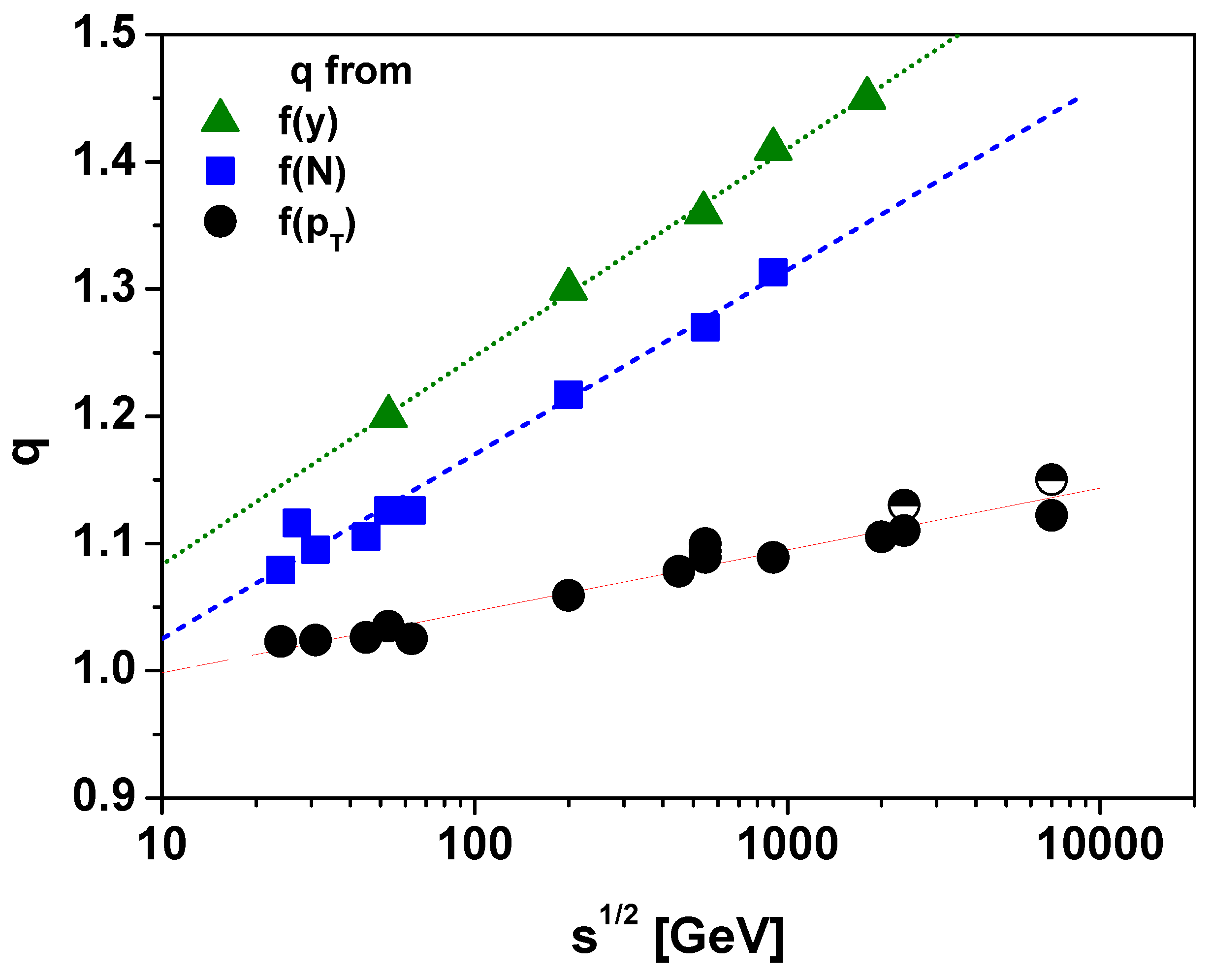
In most cases, it is this form of distribution that is used phenomenologically to describe the various distributions measured in high-energy multiple particle production experiments (with and the scaling factor T is usually identified with the temperature and X denotes the energy or momentum of the measured particles; it also appears in the normalization as ). As shown in Figure 1, using this form of Tsallis distribution one obtains from measurements of different observables (rapidity, multiplicity and transverse momentum) and for high enough energies (for low energies, conservation laws are important and they can sometimes push the parameter to the region). In addition, note that the values of q obtained from different observables are different (but always ). These differences are due to the influence of two factors. The first is whether is estimated from the temperature fluctuations obtained from data already averaged over other fluctuations or from data taking other fluctuations into account as well, and the second is that in different analyzes is obtained in other regions of the phase space.
However, this is not the only possible choice of constraints. Instead, using constraints in the form which seems to be more natural from the point of view of physical interpretation, namely that
obtain [16]
These two different definitions pertain to two different schemes of the nonextensive statistical mechanics [24]. It should be noted that [25] proposes a parametric technique that shows the equivalence of different schemes (including those discussed here), and [26] once again shows the relationship of both averaging schemes (i.e., Equations (10) and (11)) with duality . Now note that for
distribution from Equation (12) becomes from Equation (2) (note that in addition to the additive duality represented by Equation (13), multiplicative duality, , was also considered [27,28] shows the potential physical application of a combination of both types of duality to study cosmic ray physics). This means that the imposition of these constraints leads to a situation in which the non-extensiveness parameter q appearing in the definition of entropy is dual to the non-extensiveness parameter obtained from describing the observed distributions. The problem of this duality has been raised many times (for example in [29,30,31]), but it does not seem to have been put to the experimental test yet, at least not in the field of multiparticle production. It turns out, however, that experiments measuring the multiplicities and distributions of particles produced in nuclear () and nucleon () collisions are very useful for this purpose, because they simultaneously measure the multiplicities (enabling the estimation of the entropy produced) and particle distributions, and thus allow for the simultaneous determination and comparison of the non-extensiveness of the above mentioned relevant parameters and to verify the hypothesis of their duality.
Nuclear collisions are usually described by increasingly complex statistical models that try to account for all possible collective effects [32,33,34]. Because, however, for our purposes, the mutual relation between the entropies of and collisions will be important, to estimate the entropy in the nuclear collision, it will therefore be more convenient to use the phenomenological description based on the assumption that it can be described by a certain superposition of collisions of single nucleons (taking into account only nucleons that collided at least once and assuming that their collisions are independent—these are the so-called “wounded nucleons”) [35]. (The reason for this choice may be the fact that, despite its apparent simplicity, this model is still able to describe a surprisingly large number of experimental results [36,37]).
In this approach, the total observed multiplicity N is the sum of the multiplicities of particles emitted from individual sources, and the average total multiplicity is the product of the average number of sources, , and the average multiplicity from the source, , (which here is assumed to be the same for each source):
The identity of the sources assumed here means that their entropies are equal, so using the relationship (4) the entropy of such sources is
In further considerations, will denote the number of nucleons of the incident nucleus participating in the collision (i.e., participants), and , where is the number of wounded nucleons. Continuing in the same vein and assuming that the total entropy is proportional to the average multiplicity of particles produced in the collision,
we can relate the average multiplicities in nuclear () and nucleon () collisions, namely
This simple dependence already allows for some preliminary assessment of the q parameter. It turns out that the observed grows non-linearly with , [38]. Considering this observation from the point of view of entropy, it is clear that we must have here.
However, this is only a very rough estimate, because, strictly speaking, formula (17) is not fully correct with respect to the entropy. We will therefore return to Equation (15) denoting now the entropy for the whole particle production process by s and the corresponding non-extensiveness parameter by , and their equivalents for nucleon collisions by S and q, respectively. The relation (15) for N particles now looks like this:
where is the entropy for a single particle. In the collision with nucleons participating Equation (15) results in
where is the entropy for a single nucleon. Denoting multiplicity in single collisions by n, one can write that the respective entropy is
whereas the entropy in collisions for N produced particles is
This means therefore that
Parameters q and are usually not the same. However, from analyzes in [38,39] one obtains that for collisions (where ) . On the other hand, for Equation (22) corresponds to the situation encountered in superpositions as now one obtains
In the general case, we obtain the formula for the ratio )
where
which for , and is presented in Figure 2 for different reactions (see [40] for more details). Note that for energies GeV one has . This means that and (because ) also , confirming therefore previous estimates based on Equation (17).
This, however, is as much as can be said for sure, because while the distributions can give exact values of the parameter , the same cannot be said about q except that (at least in a certain energy range). We still have too many free parameters here, e.g., unknown a priori entropy . Therefore, while the statement that mostly we have and seems certain, it is not known how exactly (if at all) the duality (13) is satisfied.
3. More Thorough Screening of Duality
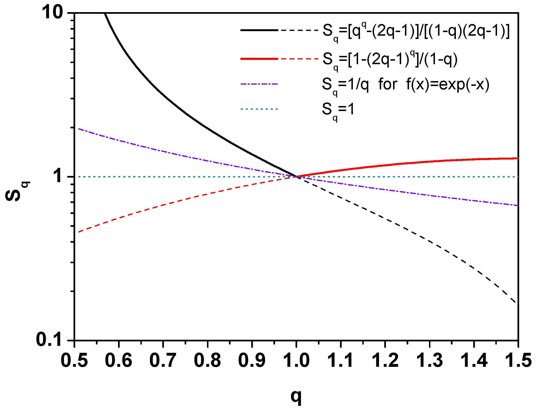
We will now deal with the problem of duality in more detail. Figure 3 shows the entropies obtained from the distributions (12) for ,
(here, was changed to ), and for ,
Let us note that for values of q outside the range of variability declared for a given entropy, , i.e., it is always lower than unity, which is less than the Shannon entropy. From Figure 3 it can be seen that the entropy formula , which could be used in the entire allowable range of the parameter q, describing both q cases and dual to them, must contain both elements of (26) and (27), i.e., have the following form:
The corresponding Tsallis distribution is now
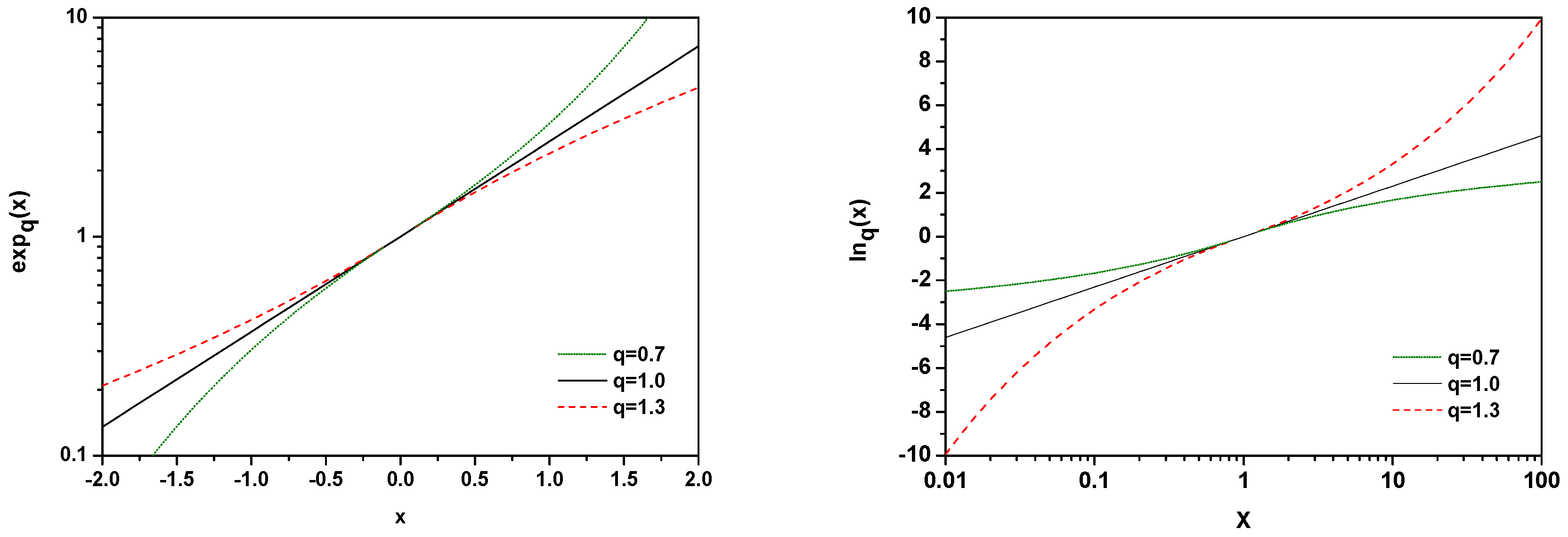
A natural question arises as to what should be modified and how in such a case? What we would like to suggest here is the use of appropriately modified definitions of the and functions, namely to replace defined in Equation (2) by
and, accordingly,
This form works for all x and q values, and there are no additional restrictions on the admissible values of the q parameter depending on whether or . Formally, this corresponds to replacing when changing the sign of x. Figure 4 shows behaviour of the functions and . Note that using this form we now have
and the ocupation numbers of particles and antiparticles satisfy relation
for all values of q ( for bosons and for fermions). The naive replecement of the Euler-exponential with another, deformed exponential function (namely given by Equation (2)) can lose the particle-hole symmetry, inherent in the traditional Fermi distribution above and below the Fermi level. Previously, these relationships had a dual form,
This means that such an approach avoids not only the problem of duality discussed earlier in Section 2, but also preserves the particle-hole symmetry concerning distribution above and below the Fermi level which is fundamental in field theory and was discussed in [42,43].
In the above considerations, we must remember that the modified functions and are not differentiable everywhere because the functions (in the first case) and (in the second) have a discontinuity at or . Therefore, by their derivatives for (or ), we understand their limits for (or ). In this approach, the first derivatives and are the same for and as the first derivatives and , while their n-th derivatives already depend on q in the following way:
and
4. Other Sources of Tsallis Distribution
Note that since Equation (2) describes the data in the entire measured area of phase space, i.e., both those associated with the thermal approach and those associated with hard collisions, the justification of this formula cannot be reduced to the Tsallis entropy only. It is worth noting that for each probability distribution the appropriate form of entropy can be given and for each probability distribution one can also give the constraints which, when used together with the Shannon entropy, lead to this probability distribution [44]. For our considerations, it is important to note that when selecting the constraints in such a way that they best take into account the most important dynamic features of the examined system, one could basically stop at the Shannon entropy [45]. For example, condition provides to the usual exponential distribution, gives Gaussian distribution, gamma distribution, whereas gives a Cauchy distribution. In general, for some function , the maximum entropy density for satisfying the constraint has the form where parameters and are fixed by the requirement of normalization for and by the above constraint. To obtain the Tsallis distribution in this way,
we need to use a constraint like this:
The Tsallis distribution understood as a quasi-power distribution can also be obtained in many ways without referring to any form of entropy [46]. We will now discuss a few of them in more detail.
Superstatistics. This approach extends the exponential description, , characterized by some parameter of the scale, T, by allowing fluctuations of this parameter [47]. In particular, if they are described by a gamma distribution,
the total result is a Tsallis distribution [29,48], the , where the parameter q characterizing the strength of fluctuations in T is given by its variance, . Since in thermal models is related to the heat capacity , one possible meaning of the parameter q is its relationship to the heat capacity, (note that here always). Other classes of generalized statistics can also be obtained, and with small variance of fluctuations they all behave universally [47].
Preferential attachment. This approach describes a situation where the scale parameter depends linearly on the variable under consideration, as is the case when preferential attachment correlations are encountered in the system under consideration, e.g., when . This changes the equation defining the distribution, resulting in the Tsallis distribution with [49,50],
Tsallis distribution from multiplicative noise. The Tsallis distribution may also mean that the described process has a stochastic character defined by the additive, , and multiplicative, , noise and described by the Langevin equation,
The corresponding Fokker-Planck equation has the form
and for stationary solutions
When both noises are uncorrelated (i.e., when ) and when there is no drift caused by additive noise (i.e., ) the solution to Equation (44) is the Tsallis distribution in [51]:
The Tsallis distribution with p (as in Equation (2)) and not is obtained for the more complicated case of when [46]
Note that T now depends non-linearly on q, which significantly makes the Tsallis distribution more flexible, allowing for the analysis and comparison of various types of processes (cf. [46]).
At this point, it is worth noting that there is a relationship between the type of noise and the condition imposed in MaxEnt. In the case of Shannon entropy, a condition imposed on the arithmetic mean corresponds to additive noise, while the use of a condition imposed on the geometric mean corresponds to multiplicative noise and leads to a power distribution [52].
Conditional probability. The methods for obtaining the Tsallis distribution presented so far are basically limited to cases with . Cases with can only be observed in constrained systems. Consider for example N independent energies, , where each of them follows the Boltzman distribution, , and their sum, , has a gamma distribution, . However, if the available energy is bounded, , these energies will no longer be independent and will be described by conditional probabilities in the form of Tsallis distributions with :
One could obtain a Tsallis-like distribution with only if the scale parameter fluctuates in the same way as in the case of superstatistics.
Statistical physics. A Tsallis distribution with also follows from statistical physics. Consider an isolated system with energy and degrees of freedom (particles). We choose one of them with energy , then the rest of the system has energy . If this particle is in one well-defined state then the number of states of the entire system is , and the probability that the energy of the selected particle is E is . Expanding around U and keeping only the first two terms one obtains
that is a Boltzman distribution with
However, it is usually expected that with . Choosing and (because the number of states in the reservoir has decreased by one), therefore
This allows us to write the probability of selection of energy E as:
that is, in the form of the Tsallis distribution with , such as in the case of conditional probability above.
5. Summary and Conclusions
Entropy has always played an important role in the study of the production mechanisms of particles produced in high-energy hadronic and nuclear collisions, either in their description based on thermodynamics [2] or in descriptions using elements of information theory [4].
In the application of the non-extensive approach, we encounter the problem of a certain duality manifested in the parallel occurrence of the parameter q and , which is best illustrated by the parallel description of particle production processes in nucleon and nuclear collisions discussed in Section 2. The second manifestation of duality appears in an attempt at a non-extensive description of quantum statistical distributions. As suggested by the results of [42,43] they are inconsistent with the conventional description using Tsallis distributions (and prefer the nonextensive Kaniadakis distribution). The point here is the necessity to preserve the particle-hole symmetry requiring that , while using the original q-exponential Tsallis distribution it leads to . In Section 3 we propose a new formula defining the non-extensive function which restores this symmetry and we have a nonextensive version of particle-hole symmetry again which restores this symmetry in the form .
From a more technical perspective, it is worth noting that both Shannon’s and Tsallis’ entropies have the same generating function, , and that the difference in their forms is just due to the form of adopted differentiation operator. For standard first-order differentiation, , we obtain the Shannon entropy, whereas adopting the Jackson q-derivative, , yields the Tsallis entropy. In fact, other expressions for entropy can be obtained by using yet other forms of differentiation operators [7].
Author Contributions
G.W. and Z.W. contributed equally to all stages of this work: conceived the problem, calculations and preparation of the manuscript. All authors have read and agreed to the published version of the manuscript.
Funding
This research was supported in part by the Polish Ministry of Education and Science, grant Nr 2022/WK/01.(GW).
Institutional Review Board Statement
Not applicable.
Data Availability Statement
Not applicable.
Acknowledgments
We would like to thank warmly Nicholas Keeley for reading the manuscript.
Conflicts of Interest
The authors declare no conflict of interest.
References
- Kittel, W.; De Wolf, E.A. Multihadron Dynamics; World Scientific: Singapore, 2005. [Google Scholar]
- Schlögl, F. Probability and Heat—Fundamentals of Thermostatistics; Springer Fachmedien Wiesbaden GmbH: Wiesbaden, Germany, 1989. [Google Scholar]
- Biró, T.S. Is there a Temperature? Conceptual Challenges at High Energy, Acceleration and Complexity; Springer: New York, NY, USA; Dordrecht, The Netherlands; Heidelberg, Germany; London, UK, 2011. [Google Scholar]
- Arndt, C. Information Measures—Information and its Description in Science and Engineering; Springer: Berlin/Heidelberg, Germany; New York, NY, USA, 2001. [Google Scholar]
- Tsallis, C. Introduction to Nonextensive Statistical Mechanics; Springer: New York, NY, USA, 2009. [Google Scholar]
- Naudts, J. Generalised Thermostatistics; Springer: London, UK; Dordrecht, The Netherlands; Heidelberg, Germany; New York, NY, USA, 2011. [Google Scholar]
- Lopes, A.M.; Machado, J.A. A Review of Fractional Order Entropies. Entropy 2020, 22, 1374. [Google Scholar] [CrossRef] [PubMed]
- Havrda, J.; Charvat, F. Quantification Method of Classification Processes—Concept of Structural α-Entropy. Kybernetica 1967, 3, 30–34. [Google Scholar]
- Daroczy, Z. Generalized information functions. Inf. Control 1970, 16, 36–51. [Google Scholar] [CrossRef] [Green Version]
- Wilk, G.; Włodarczyk, Z. Example of a possible interpretation of Tsallis entropy. Phys. A 2008, 387, 4809–4813. [Google Scholar] [CrossRef] [Green Version]
- Neuman, Y.; Cohen, Y.; Neuman, Y. How to (better) find a perpetrator in a haystack. J. Big Data 2019, 6, 1–17. [Google Scholar] [CrossRef] [Green Version]
- Michael, C.; Vanryckeghem, L. Consequences of momentum conservation for particle production at large transverse momentum. J. Phys. G 1977, 3, L151–L156. [Google Scholar] [CrossRef]
- Michael, C. Large transverse momentum and large mass production in hadronic interactions. Prog. Part. Nucl. Phys. 1979, 2, 1–39. [Google Scholar] [CrossRef]
- Hagedorn, R. Multiplicities, pT Distributions and the Expected Hadron → Quark-Gluon Phase Transition. Riv. Nuovo Cim. 1983, 6, 1–50. [Google Scholar] [CrossRef]
- Abe, S. Nonadditive conditional entropy and its significance for local realism. Phys. A 2001, 289, 157–164. [Google Scholar] [CrossRef] [Green Version]
- Rathie, P.N.; Da Silva, S. Shannon, Lévy, and Tsallis: A Note. Appl. Math. Sci. 2008, 2, 1359–1363. [Google Scholar]
- Dash, A.K.; Mohanty, B.M. Extrapolation of multiplicity distribution in p + p() collisions to LHC energies. J. Phys. G 2010, 37, 025102. [Google Scholar] [CrossRef] [Green Version]
- Geich-Gimbel, C. Particle production at collider energies. Int. J. Mod. Phys. A 1989, 4, 1527–1680. [Google Scholar] [CrossRef]
- Wibig, T. The non-extensivity parameter of a thermodynamical model of hadronic interactions at LHC energies. J. Phys. G 2010, 37, 115009. [Google Scholar] [CrossRef] [Green Version]
- Khachatryan, V.; Sirunyan, A.M.; Tumasyan, A.; Adam, W.; Bergauer, T.; Dragicevic, M.; Erö, J.; Friedl, M.; Fruehwirth, R.; Ghete, V.M.; et al. Transverse-momentum and pseudorapidity distributions of charged hadrons in pp collisions at = 0.9 and 2.36 TeV. J. High Energ. Phys. 2010, 2, 41. [Google Scholar] [CrossRef] [Green Version]
- Khachatryan, V.; Sirunyan, A.M.; Tumasyan, A.; Adam, W.; Bergauer, T.; Dragicevic, M.; Erö, J.; Fabjan, C.; Friedl, M.; Fruehwirth, R.; et al. Transverse-Momentum and Pseudorapidity Distributions of Charged Hadrons in pp Collisions at = 7 TeV. Phys. Rev. Lett. 2010, 105, 022002. [Google Scholar] [CrossRef] [Green Version]
- Navarra, F.S.; Utyuzh, O.V.; Wilk, G.; Włodarczyk, Z. Information theory approach (extensive and nonextensive) to high-energy multiparticle production processes. Phys. A 2004, 340, 467–476. [Google Scholar] [CrossRef] [Green Version]
- Rybczyński, M.; Włodarczyk, Z.; Wilk, G. Rapidity spectra analysis in terms of non-extensive statistic approach. Nucl. Phys. B (Proc. Suppl.) 2003, 122, 325–328. [Google Scholar] [CrossRef] [Green Version]
- Tsallis, C.; Mendes, R.S.; Plastino, A.R. The role of constraints within generalized nonextensive statistics. Physica A 1998, 261, 534–554. [Google Scholar] [CrossRef]
- Ferri, G.L.; S Martínez, S.; Plastino, A. Equivalence of the four versions of Tsallis’s statistics. J. Stat. Mech. 2005, P04009, 1–14. [Google Scholar] [CrossRef] [Green Version]
- Parvan, A.S. Equivalence of the phenomenological Tsallis distribution to the transverse momentum distribution of q-dual statistics. Eur. Phys. J. A 2020, 56, 106. [Google Scholar] [CrossRef]
- Tsallis, C. On the foundations of statistical mechanics. Eur. Phys. J. Spec. Topics 2017, 226, 1433–1443. [Google Scholar] [CrossRef] [Green Version]
- Yalcin, G.C.; Beck, C. Generalized statistical mechanics of cosmic rays: Application to positron-electron spectral indices. Sci. Rep. 2018, 8, 1764. [Google Scholar] [CrossRef] [PubMed] [Green Version]
- Biró, T.S.; Jakovác, A. Power-Law Tails from Multiplicative Noise. Phys. Rev. Lett. 2005, 94, 132302. [Google Scholar] [CrossRef] [Green Version]
- Biró, T.S.; Purcel, G.; Ürmösy, K. Non-extensive approach to quark matter. Eur. Phys. J. A 2009, 40, 325–340. [Google Scholar]
- Karlin, I.V.; Grmela, M.; Gorban, N. Duality in nonextensive statistical mechanics. Phys. Rev. E 2002, 65, 036128. [Google Scholar] [CrossRef] [Green Version]
- Gaździcki, M.; Gorenstein, M.; Seybothe, P. Onset of Deconfinement in Nucleus–Nucleus Collisions: Review for Pedestrians and Experts. Acta Phys. Polon. B 2011, 42, 307–351. [Google Scholar] [CrossRef]
- Gaździcki, M.; Rybicki, A. Overview of results from NA61/SHINE: Uncovering critical structures. Acta Phys. Polon. B 2019, 50, 1057–1070. [Google Scholar] [CrossRef]
- Noronha, J. Collective effects in nuclear collisions: Theory overview. Nucl. Phys. A 2019, 982, 78–84. [Google Scholar] [CrossRef]
- Białas, A.; Błeszynski, M.; Czyż, W. Multiplicity distributions in nucleus-nucleus collisions at high energies. Nucl. Phys. B 1976, 111, 461–476. [Google Scholar] [CrossRef]
- Fiałkowski, K.; Wit, R. RHIC Multiplicity Distributions and Superposition Models. Acta Phys. Pol. B 2010, 41, 1317–1325. [Google Scholar]
- Fiałkowski, K.; Wit, R. Superposition models and the multiplicity fluctuations in heavy-ion collisions. Eur. Phys. J. A 2010, 45, 51–55. [Google Scholar] [CrossRef]
- Wilk, G.; Włodarczyk, Z. Multiplicity fluctuations due to the temperature fluctuations in high-energy nuclear collisions. Phys. Rev. C 2009, 79, 054903. [Google Scholar] [CrossRef] [Green Version]
- Shao, M.; Yi, L.; Tang, Z.; Chen, H.; Li, C.; Xu, Z. Examination of the species and beam energy dependence of particle spectra using Tsallis statistics. J. Phys. G 2010, 37, 085104. [Google Scholar] [CrossRef]
- Wilk, G.; Włodarczyk, Z. The imprints of superstatistics in multiparticle production processes. Cent. Eur. J. Phys. 2012, 10, 568–575. [Google Scholar] [CrossRef] [Green Version]
- Backet, B.B.; Baker, M.D.; Barton, D.S.; Betts, R.R.; Ballintijn, M.; Bickley, A.A.; Bindel, R.; Budzanowski, A.; Busza, W.; Carroll, A.; et al. Centrality and energy dependence of charged-particle multiplicities in heavy ion collisions in the context of elementary reactions. Phys. Rev. C 2006, 74, 021902. [Google Scholar] [CrossRef]
- Biró, T.S.; Shen, K.M.; Zhang, B.W. Non-extensive quantum statistics with particle–hole symmetry. Phys. A 2015, 428, 410–415. [Google Scholar] [CrossRef] [Green Version]
- Biró, T.S. Kaniadakis Entropy Leads to Particle–Hole Symmetric Distribution. Entropy 2022, 24, 1217. [Google Scholar] [CrossRef]
- Papalexiou, S.M.; Koutsoyiannis, D. Entropy Maximization, P-Moments and Power-Type Distributions in Nature. Available online: http://itia.ntua.gr/1127 (accessed on 8 April 2011).
- Rufeil Fiori, E.; Plastino, A. A Shannon–Tsallis transformation. Phys. A 2013, 392, 1742–1749. [Google Scholar]
- Wilk, G.; Włodarczyk, Z. Quasi-power law ensembles. Acta Phys. Pol. B 2015, 46, 1103–1122. [Google Scholar] [CrossRef] [Green Version]
- Beck, C.; Cohen, E.G.D. Superstatistics. Phys. A 2003, 322, 267–275. [Google Scholar] [CrossRef] [Green Version]
- Wilk, G.; Włodarczyk, Z. Interpretation of the Nonextensivity Parameter q in Some Applications of Tsallis Statistics and Lévy Distributions. Phys. Rev. Lett. 2000, 84, 2770–2773. [Google Scholar] [CrossRef] [PubMed] [Green Version]
- Wilk, G.; Włodarczyk, Z. Nonextensive information entropy for stochastic networks. Acta Phys. Pol. B 2004, 35, 871–879. [Google Scholar]
- Soares, D.J.B.; Tsallis, C.; Mariz, A.M.; da Silva, L.R. Preferential attachment growth model and nonextensive statistical mechanics. Europhys. Lett. 2005, 70, 70–76. [Google Scholar] [CrossRef] [Green Version]
- Anteneodo, C.; Tsallis, C. Multiplicative noise: A mechanism leading to nonextensive statistical mechanics. J. Math. Phys. 2003, 44, 5194–5203. [Google Scholar] [CrossRef] [Green Version]
- Rostovtsev, A. On a geometric mean and power-law statistical distributions. arXiv 2005, arXiv:cond-mat/0507414. [Google Scholar]
Figure 1.
(Color online) Energy dependencies of the parameters q obtained from different observables. Squares: q obtained from multiplicity distributions [17,18] (fitted by ). Circles: q obtained from different analyses of the transverse momenta distribution . Data points are, respectively, from a compilation of data (full symbols) [19], from CMS data (half filled circles at high energies) [20,21] (fitted by . Triangles: q obtained from analyses of rapidity distributions [22,23] (and fitted by .

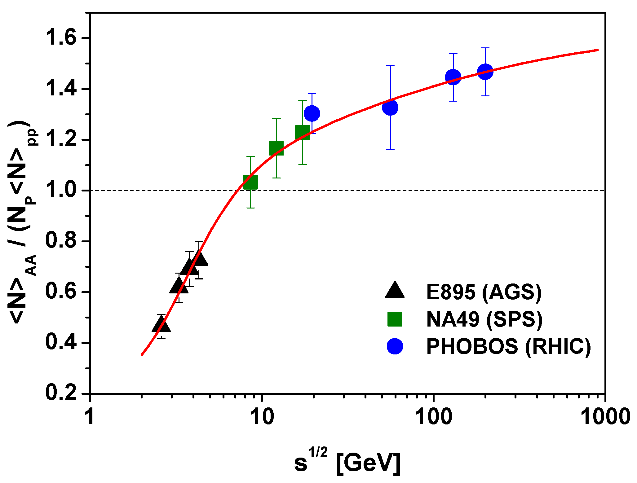
Figure 2.
(Color online) Energy dependence of the charged multiplicity for nucleus-nucleus collisions divided by the superposition of multiplicities from proton-proton collisions using Equation (24) with and with depending on energy according to . Experimental data on multiplicity are taken from the compilation of Ref. [41].

Figure 3.
(Color online) Tsallis entropy for different nonextensivity parameter (see text for details).
Figure 3.
(Color online) Tsallis entropy for different nonextensivity parameter (see text for details).


Disclaimer/Publisher’s Note: The statements, opinions and data contained in all publications are solely those of the individual author(s) and contributor(s) and not of MDPI and/or the editor(s). MDPI and/or the editor(s) disclaim responsibility for any injury to people or property resulting from any ideas, methods, instructions or products referred to in the content. |
© 2023 by the authors. Licensee MDPI, Basel, Switzerland. This article is an open access article distributed under the terms and conditions of the Creative Commons Attribution (CC BY) license (https://creativecommons.org/licenses/by/4.0/).
Share and Cite
MDPI and ACS Style
Wilk, G.; Włodarczyk, Z. Some Non-Obvious Consequences of Non-Extensiveness of Entropy. Entropy 2023, 25, 474. https://doi.org/10.3390/e25030474
AMA Style
Wilk G, Włodarczyk Z. Some Non-Obvious Consequences of Non-Extensiveness of Entropy. Entropy. 2023; 25(3):474. https://doi.org/10.3390/e25030474
Chicago/Turabian StyleWilk, Grzegorz, and Zbigniew Włodarczyk. 2023. "Some Non-Obvious Consequences of Non-Extensiveness of Entropy" Entropy 25, no. 3: 474. https://doi.org/10.3390/e25030474
Note that from the first issue of 2016, this journal uses article numbers instead of page numbers. See further details here.