
System Integrated Information

 , , , , , , , and
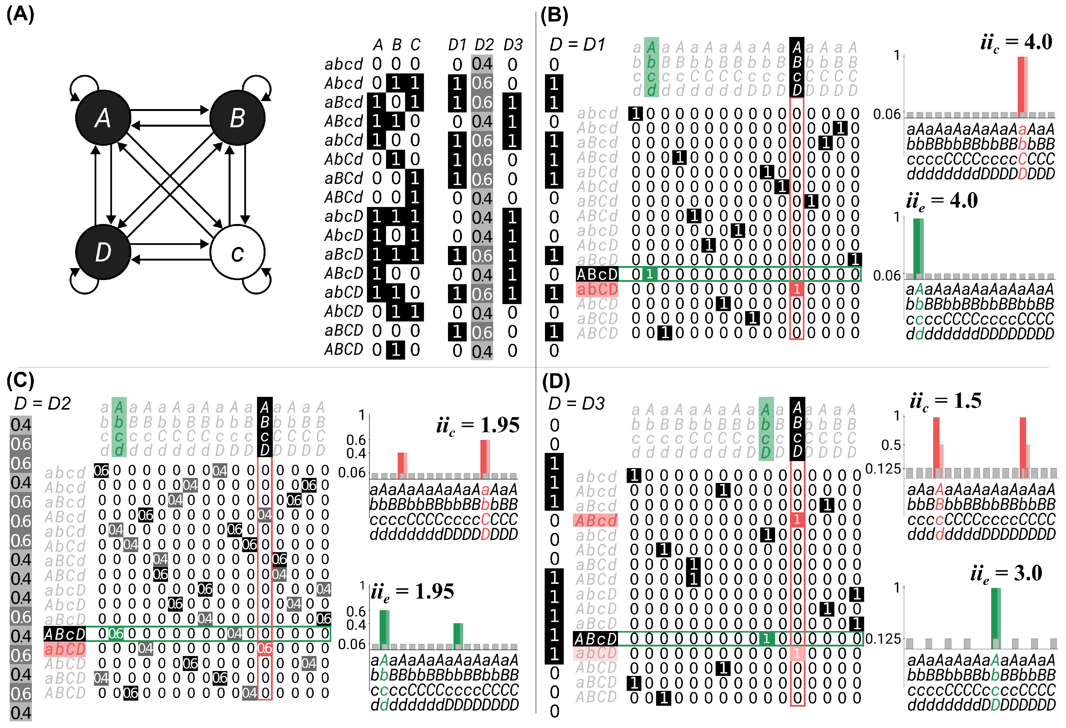
Abstract
:1. Introduction
- Intrinsicality
- Experience is intrinsic: it exists for itself.
- Information
- Experience is specific: it is the way it is.
- Integration
- Experience is unitary: it is a whole, irreducible to separate experiences.
- Exclusion
- Experience is definite: it is this whole.
- Composition
- Experience is structured: it is composed of distinctions and the relations that bind them together, yielding a phenomenal structure.
- Intrinsicality
- The substrate of consciousness must have intrinsic cause–effect power: it must take and make a difference within itself.
- Information
- The substrate of consciousness must have specific cause–effect power: it must select a specific cause–effect state.
- Integration
- The substrate of consciousness must have unitary cause–effect power: it must specify its cause–effect state as a whole set of units, irreducible to separate subsets of units.
- Exclusion
- The substrate of consciousness must have definite cause–effect power: it must specify its cause–effect state as this set of units.
- Composition
- The substrate of consciousness must have structured cause–effect power: subsets of its units must specify cause–effect states over subsets of units (distinctions) that can overlap with one another (relations), yielding a cause–effect structure.
2. Theory
2.1. Intrinsicality
2.2. Information
2.3. Integration
2.4. Exclusion
3. Results and Discussion
3.1. Example 1: Information
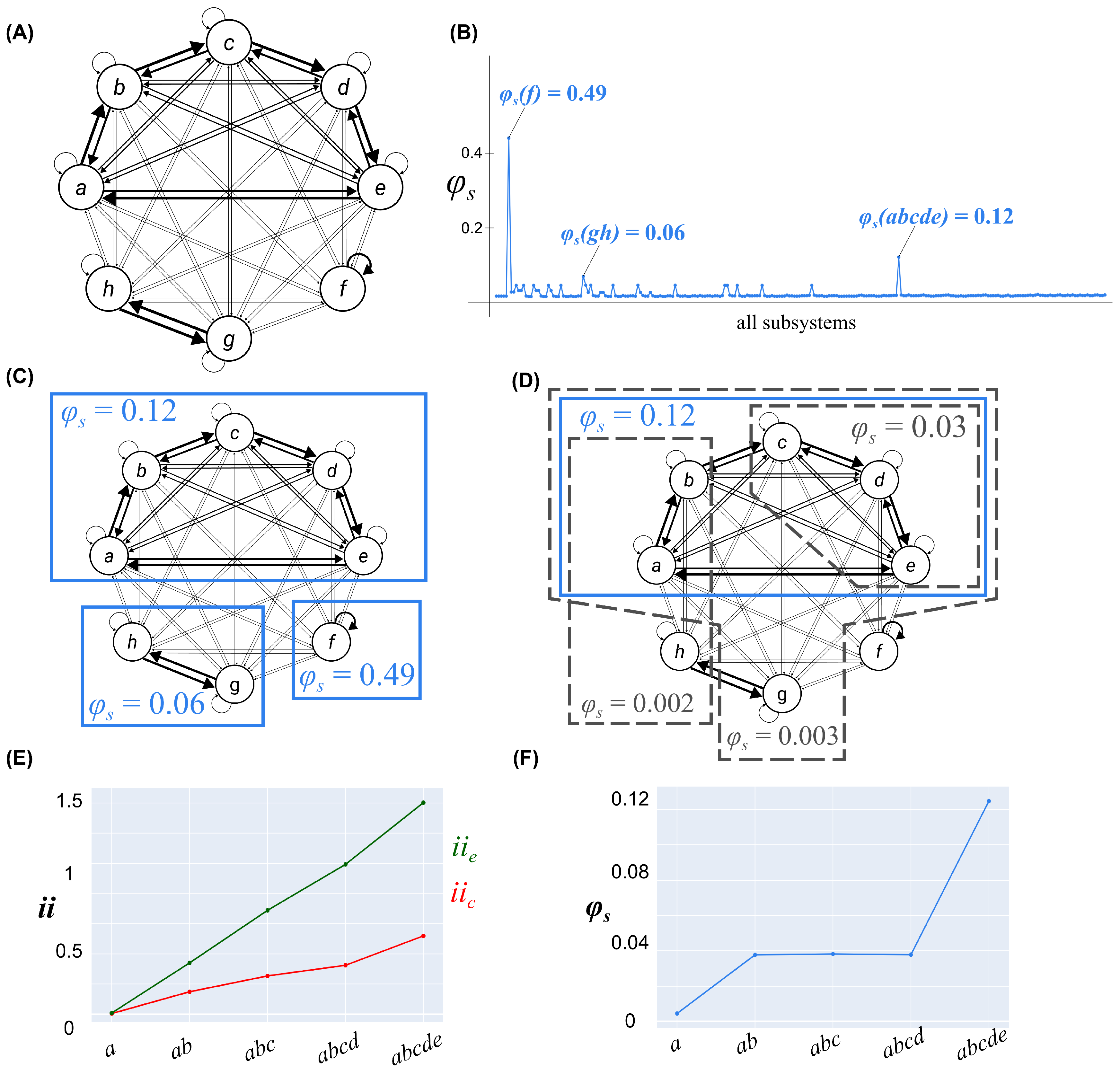
3.2. Example 2: Integration
3.3. Example 3: Exclusion
4. Conclusions
Author Contributions
Funding
Conflicts of Interest
Appendix A. Computations
Appendix A.1. Cause–Effect Repertoires
Appendix A.2. System Partition
Appendix B. Proof of Theorem 1
Appendix C. Recursive PSC Algorithm
| Algorithm A1 An algorithm for carving a universe U into a set of non-overlapping complexes |
|
References
- Tononi, G.; Boly, M.; Massimini, M.; Koch, C. Integrated information theory: From consciousness to its physical substrate. Nat. Rev. Neurosci. 2016, 17, 450–461. [Google Scholar] [CrossRef]
- Tononi, G.; Koch, C. Consciousness: Here, there and everywhere? Philos. Trans. R. Soc. B Biol. Sci. 2015, 370, 20140167. [Google Scholar] [CrossRef] [PubMed]
- Albantakis, L.; Barbosa, L.; Findlay, G.; Grasso, M.; Haun, A.M.; Marshall, W.; Mayner, W.G.; Zaeemzadeh, A.; Boly, M.; Juel, B.E.; et al. Integrated information theory 4.0: A comprehensive overview. arXiv 2022, arXiv:2212.14787. [Google Scholar] [CrossRef]
- Tononi, G. Integrated information theory. Scholarpedia 2015, 10, 4164. [Google Scholar] [CrossRef]
- Oizumi, M.; Albantakis, L.; Tononi, G. From the phenomenology to the mechanisms of consciousness: Integrated information theory 3.0. PLoS Comput. Biol. 2014, 10, e1003588. [Google Scholar] [CrossRef]
- Barbosa, L.S.; Marshall, W.; Albantakis, L.; Tononi, G. Mechanism integrated information. Entropy 2021, 23, 362. [Google Scholar] [CrossRef]
- Balduzzi, D.; Tononi, G. Integrated information in discrete dynamical systems: Motivation and theoretical framework. PLoS Comput. Biol. 2008, 4, e1000091. [Google Scholar] [CrossRef]
- Tononi, G. An information integration theory of consciousness. BMC Neurosci. 2004, 5, 42. [Google Scholar] [CrossRef]
- Barbosa, L.S.; Marshall, W.; Streipert, S.; Albantakis, L.; Tononi, G. A measure for intrinsic information. Sci. Rep. 2020, 10, 1–9. [Google Scholar] [CrossRef] [PubMed]
- Haun, A.; Tononi, G. Why does space feel the way it does? Towards a principled account of spatial experience. Entropy 2019, 21, 1160. [Google Scholar] [CrossRef] [Green Version]
- Albantakis, L.; Tononi, G. Causal composition: Structural differences among dynamically equivalent systems. Entropy 2019, 21, 989. [Google Scholar] [CrossRef]
- Albantakis, L.; Marshall, W.; Hoel, E.; Tononi, G. What caused what? A quantitative account of actual causation using dynamical causal networks. Entropy 2019, 21, 459. [Google Scholar] [CrossRef] [PubMed]
- Mayner, W.; Marshall, W.; Albantakis, L.; Findlay, G.; Marchman, R.; Tononi, G. PyPhi: A toolbox for integrated information theory. PLoS Comput. Biol. 2018, 14, e1006343. [Google Scholar] [CrossRef] [PubMed]
- Tononi, G.; Sporns, O.; Edelman, G.M. Measures of degenearcy and redundancy in biological networks. Proc. Natl. Acad. Sci. USA 1999, 96, 3257–3262. [Google Scholar] [CrossRef] [PubMed]
- Hoel, E.P.; Albantakis, L.; Tononi, G. Quantifying causal emergence shows that macro can beat micro. Proc. Natl. Acad. Sci. USA 2013, 110, 19790–19795. [Google Scholar] [CrossRef]
- Hoel, E.P.; Albantakis, L.; Marshall, W.; Tononi, G. Can the macro beat the micro? Integrated information across spatiotemporal scales. Neurosci. Conscious. 2016, 2016, niw012. [Google Scholar] [CrossRef]
- Albantakis, L.; Hintze, A.; Koch, C.; Adami, C.; Tononi, G. Evolution of integrated causal structures in animats exposed to environments of increasing complexity. PLoS Comput. Biol. 2014, 10, e1003966. [Google Scholar] [CrossRef]
- Safron, A. Integrated world modeling theory expanded: Implications for the future of consciousness. Front. Comput. Neurosci. 2022, 16, 642397. [Google Scholar] [CrossRef]
- Olesen, C.; Waade, P.; Albantakis, L.; Mathys, C. Phi fluctuates with surprisal: An empirical pre-study for the synthesis of the free energy principle and integrated information theory. PsyArXiv 2023. [Google Scholar] [CrossRef]
- Edlund, J.A.; Chaumont, N.; Hintze, A.; Koch, C.; Tononi, G.; Adami, C. Integrated information increases with fitness in the evolution of animats. PLoS Comput. Biol. 2011, 7, e1002236. [Google Scholar] [CrossRef] [Green Version]
- Joshi, N.; Tononi, G.; Koch, C. The minimal complexity of adapting agents increases with fitness. PLoS Compuational Biol. 2013, 9, e1003111. [Google Scholar] [CrossRef] [PubMed]
- Marshall, W.; Kim, H.; Walker, S.I.; Tononi, G.; Albantakis, L. How causal analysis can reveal autonomy in models of biological systems. Philos. Trans. R. Soc. A 2017, 375, 20160358. [Google Scholar] [CrossRef] [PubMed]
- Marshall, W.; Albantakis, L.; Tononi, G. Black-boxing and cause-effect power. PLoS Comput. Biol. 2018, 14, e1006114. [Google Scholar] [CrossRef] [PubMed] [Green Version]


Disclaimer/Publisher’s Note: The statements, opinions and data contained in all publications are solely those of the individual author(s) and contributor(s) and not of MDPI and/or the editor(s). MDPI and/or the editor(s) disclaim responsibility for any injury to people or property resulting from any ideas, methods, instructions or products referred to in the content. |
© 2023 by the authors. Licensee MDPI, Basel, Switzerland. This article is an open access article distributed under the terms and conditions of the Creative Commons Attribution (CC BY) license (https://creativecommons.org/licenses/by/4.0/).
Share and Cite
Marshall, W.; Grasso, M.; Mayner, W.G.P.; Zaeemzadeh, A.; Barbosa, L.S.; Chastain, E.; Findlay, G.; Sasai, S.; Albantakis, L.; Tononi, G. System Integrated Information. Entropy 2023, 25, 334. https://doi.org/10.3390/e25020334
Marshall W, Grasso M, Mayner WGP, Zaeemzadeh A, Barbosa LS, Chastain E, Findlay G, Sasai S, Albantakis L, Tononi G. System Integrated Information. Entropy. 2023; 25(2):334. https://doi.org/10.3390/e25020334
Chicago/Turabian StyleMarshall, William, Matteo Grasso, William G. P. Mayner, Alireza Zaeemzadeh, Leonardo S. Barbosa, Erick Chastain, Graham Findlay, Shuntaro Sasai, Larissa Albantakis, and Giulio Tononi. 2023. "System Integrated Information" Entropy 25, no. 2: 334. https://doi.org/10.3390/e25020334