
Random Walks on Networks with Centrality-Based Stochastic Resetting


 ,
,  , and
, and
Abstract
:1. Introduction
2. Materials and Methods
2.1. Random Walk on Networks with Stochastic Resetting
2.2. Mean First Passage Time
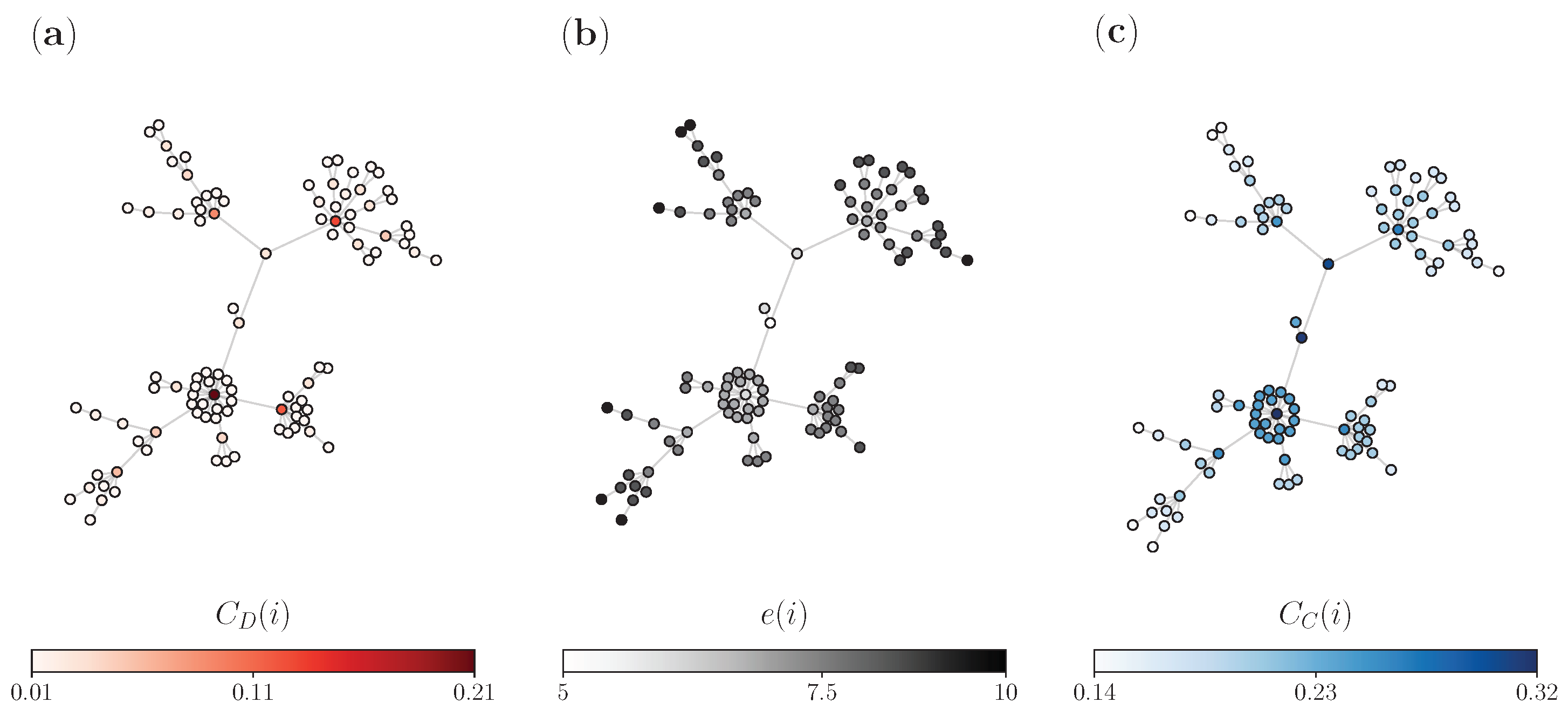
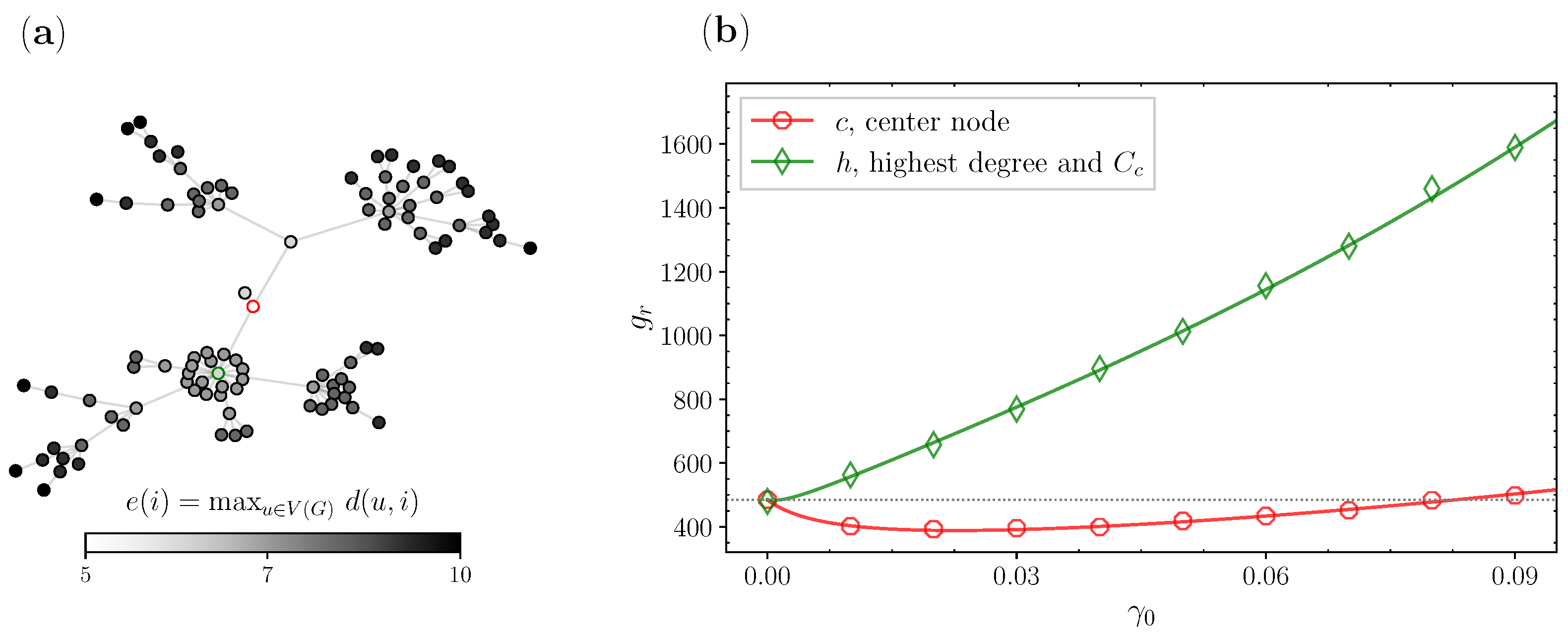
2.3. Node Centrality Approach
3. Results
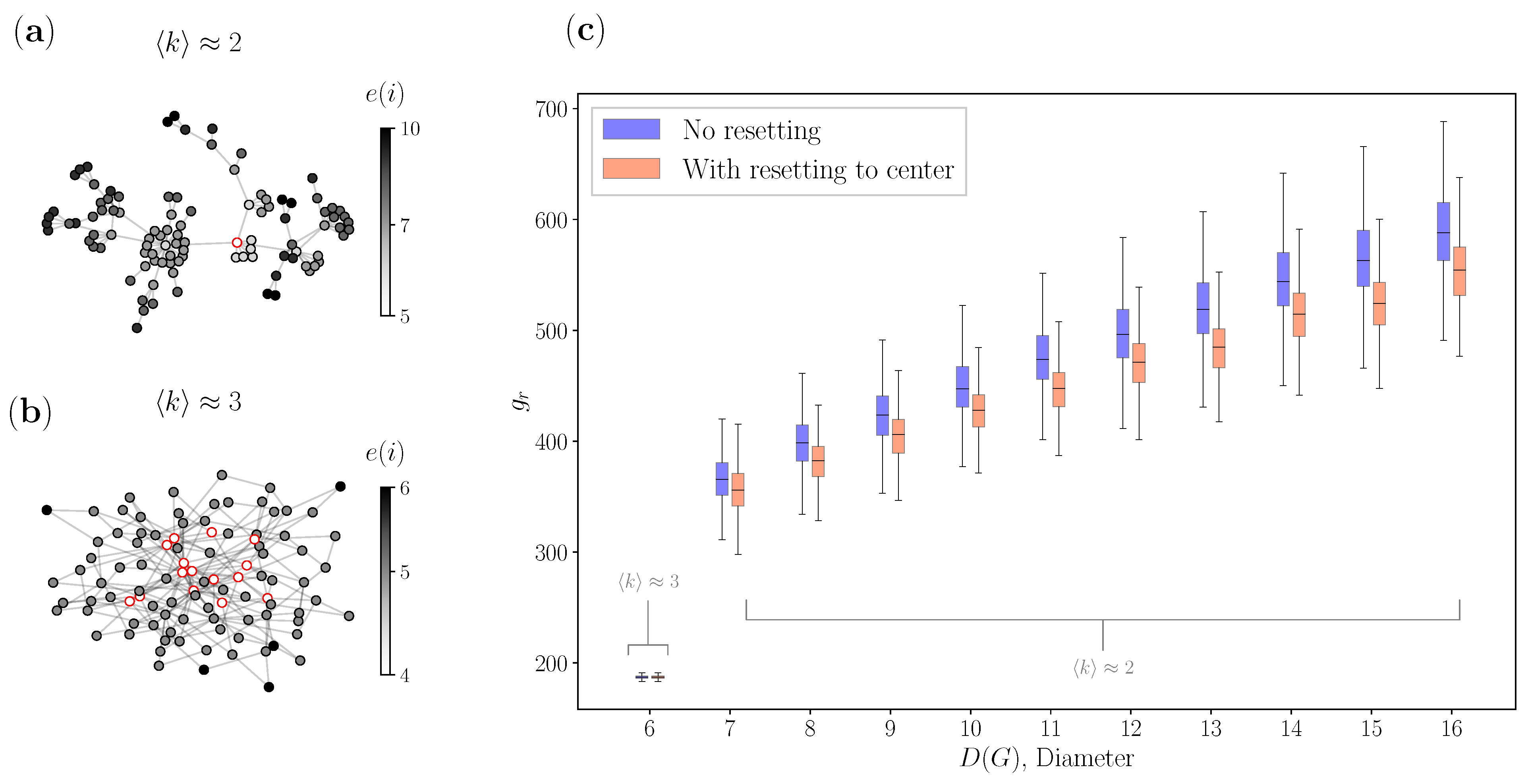
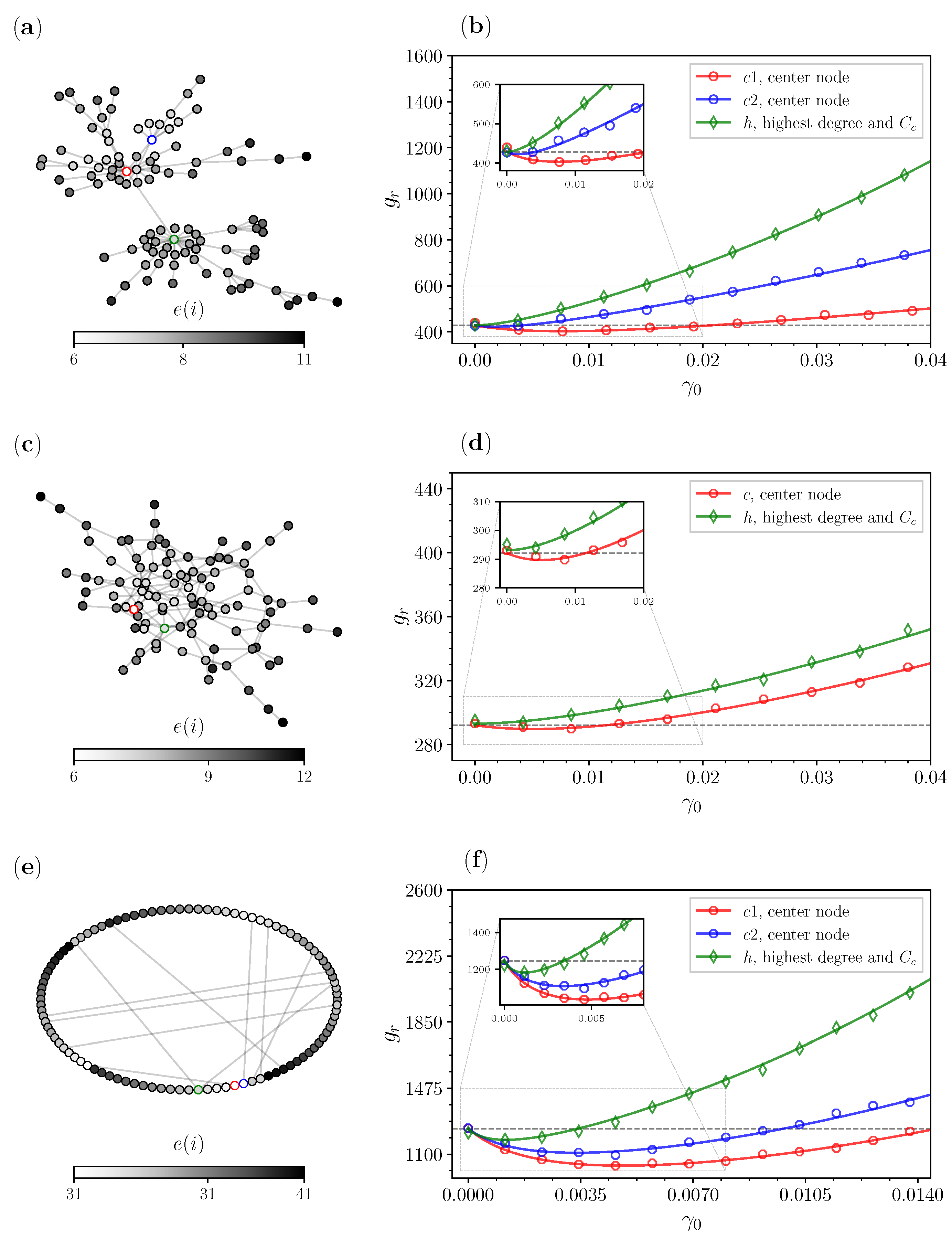
3.1. Complex Networks
3.2. Special Graphs
3.3. Real Networks
4. Conclusions
Author Contributions
Funding
Institutional Review Board Statement
Data Availability Statement
Conflicts of Interest
Abbreviations
| GMFPT | Global Mean First Passage Time |
| GMFPT | |
| FPT | First Passage Time |
| MFPT | Mean First Passage Time |
| AI | Artificial Intelligence |
| LSCC | Largest strongly connected component |
| ER | Erdos-Rényi |
| WS | Watts-Strogatz |
| BA | Barabási-Albert |
References
- Adamic, L.A.; Lukose, R.M.; Puniyani, A.R.; Huberman, B.A. Search in power-law networks. Phys. Rev. E 2001, 64, 046135. [Google Scholar] [CrossRef] [PubMed]
- Noh, J.D.; Rieger, H. Random walks on complex networks. Phys. Rev. Lett. 2004, 92, 118701. [Google Scholar] [CrossRef]
- Zhou, H. Distance, dissimilarity index, and network community structure. Phys. Rev. E 2003, 67, 061901. [Google Scholar] [CrossRef] [PubMed]
- Rosvall, M.; Bergstrom, C.T. Maps of random walks on complex networks reveal community structure. Proc. Natl. Acad. Sci. USA 2008, 105, 1118–1123. [Google Scholar] [CrossRef] [PubMed]
- Liu, W.; Lü, L. Link prediction based on local random walk. EPL (Europhys. Lett.) 2010, 89, 58007. [Google Scholar] [CrossRef]
- Brin, S.; Page, L. The anatomy of a large-scale hypertextual web search engine. Comput. Netw. ISDN Syst. 1998, 30, 107–117. [Google Scholar] [CrossRef]
- Fronczak, A.; Fronczak, P. Biased random walks in complex networks: The role of local navigation rules. Phys. Rev. E 2009, 80, 016107. [Google Scholar] [CrossRef] [PubMed]
- Basnarkov, L.; Mirchev, M.; Kocarev, L. Random walk with memory on complex networks. Phys. Rev. E 2020, 102, 042315. [Google Scholar] [CrossRef]
- Estrada, E.; Delvenne, J.C.; Hatano, N.; Mateos, J.L.; Metzler, R.; Riascos, A.P.; Schaub, M.T. Random multi-hopper model: Super-fast random walks on graphs. J. Complex Netw. 2018, 6, 382–403. [Google Scholar] [CrossRef]
- Riascos, A.P.; Boyer, D.; Herringer, P.; Mateos, J.L. Random walks on networks with stochastic resetting. Phys. Rev. E 2020, 101, 062147. [Google Scholar] [CrossRef]
- Bell, W.J. Searching Behaviour: The Behavioural Ecology of Finding Resources; Springer Science & Business Media: Berlin/Heidelberg, Germany, 2012. [Google Scholar]
- Bartumeus, F.; Catalan, J. Optimal search behavior and classic foraging theory. J. Phys. A Math. Theor. 2009, 42, 434002. [Google Scholar] [CrossRef]
- Visco, P.; Allen, R.J.; Majumdar, S.N.; Evans, M.R. Switching and growth for microbial populations in catastrophic responsive environments. Biophys. J. 2010, 98, 1099–1108. [Google Scholar] [CrossRef]
- Evans, M.R.; Majumdar, S.N. Diffusion with stochastic resetting. Phys. Rev. Lett. 2011, 106, 160601. [Google Scholar] [CrossRef] [PubMed]
- Evans, M.R.; Majumdar, S.N.; Schehr, G. Stochastic resetting and applications. J. Phys. A Math. Theor. 2020, 53, 193001. [Google Scholar] [CrossRef]
- Kusmierz, L.; Majumdar, S.N.; Sabhapandit, S.; Schehr, G. First order transition for the optimal search time of Lévy flights with resetting. Phys. Rev. Lett. 2014, 113, 220602. [Google Scholar] [CrossRef]
- Campos, D.; Méndez, V. Phase transitions in optimal search times: How random walkers should combine resetting and flight scales. Phys. Rev. E 2015, 92, 062115. [Google Scholar] [CrossRef] [PubMed]
- Pal, A.; Reuveni, S. First passage under restart. Phys. Rev. Lett. 2017, 118, 030603. [Google Scholar] [CrossRef]
- Chechkin, A.; Sokolov, I. Random search with resetting: A unified renewal approach. Phys. Rev. Lett. 2018, 121, 050601. [Google Scholar] [CrossRef]
- Dahlenburg, M.; Chechkin, A.V.; Schumer, R.; Metzler, R. Stochastic resetting by a random amplitude. Phys. Rev. E 2021, 103, 052123. [Google Scholar] [CrossRef]
- Stojkoski, V.; Sandev, T.; Basnarkov, L.; Kocarev, L.; Metzler, R. Generalised geometric Brownian motion: Theory and applications to option pricing. Entropy 2020, 22, 1432. [Google Scholar] [CrossRef]
- Bonomo, O.L.; Pal, A. First passage under restart for discrete space and time: Application to one-dimensional confined lattice random walks. Phys. Rev. E 2021, 103, 052129. [Google Scholar] [CrossRef]
- Das, D.; Giuggioli, L. Discrete space-time resetting model: Application to first-passage and transmission statistics. J. Phys. A Math. Theor. 2022, 55, 424004. [Google Scholar] [CrossRef]
- González, F.H.; Riascos, A.P.; Boyer, D. Diffusive transport on networks with stochastic resetting to multiple nodes. Phys. Rev. E 2021, 103, 062126. [Google Scholar] [CrossRef]
- Wang, S.; Chen, H.; Huang, F. Random walks on complex networks with multiple resetting nodes: A renewal approach. Chaos 2021, 31, 093135. [Google Scholar] [CrossRef] [PubMed]
- Ye, Y.; Chen, H. Random walks on complex networks under node-dependent stochastic resetting. J. Stat. Mech. 2022, 2022, 053201. [Google Scholar] [CrossRef]
- Riascos, A.P.; Boyer, D.; Mateos, J.L. Discrete-time random walks and Lévy flights on arbitrary networks: When resetting becomes advantageous? J. Phys. A Math. Theor. 2022, 55, 274002. [Google Scholar] [CrossRef]
- Wang, Y.; Chen, H. Entropy rate of random walks on complex networks under stochastic resetting. Phys. Rev. E 2022, 106, 054137. [Google Scholar] [CrossRef] [PubMed]
- Chen, H.; Ye, Y. Random walks on complex networks under time-dependent stochastic resetting. Phys. Rev. E 2022, 106, 044139. [Google Scholar] [CrossRef]
- Wuchty, S.; Stadler, P.F. Centers of complex networks. J. Theor. Biol. 2003, 223, 45–53. [Google Scholar] [CrossRef]
- Slater, P.J. On locating a facility to service areas within a network. Oper. Res. 1981, 29, 523–531. [Google Scholar] [CrossRef]
- Buckley, F. Facility location problems. Coll. Math. J. 1987, 18, 24–32. [Google Scholar] [CrossRef]
- Hage, P.; Harary, F. Eccentricity and centrality in networks. Soc. Netw. 1995, 17, 57–63. [Google Scholar] [CrossRef]
- Pavlopoulos, G.A.; Secrier, M.; Moschopoulos, C.N.; Soldatos, T.G.; Kossida, S.; Aerts, J.; Schneider, R.; Bagos, P.G. Using graph theory to analyze biological networks. BioData Min. 2011, 4, 10. [Google Scholar] [CrossRef] [PubMed]
- Krnc, M.; Sereni, J.S.; Skrekovski, R.; Yilma, Z. Eccentricity of networks with structural constraints. Discuss. Math. Graph Theory 2020, 40, 1141–1162. [Google Scholar] [CrossRef]
- Takes, F.W.; Kosters, W.A. Computing the eccentricity distribution of large graphs. Algorithms 2013, 6, 100–118. [Google Scholar] [CrossRef]
- Grinstead, C.M.; Snell, J.L. Introduction to Probability; American Mathematical Soc.: Providence, RI, USA, 2012. [Google Scholar]
- Tejedor, V.; Bénichou, O.; Voituriez, R. Global mean first-passage times of random walks on complex networks. Phys. Rev. E 2009, 80, 065104. [Google Scholar] [CrossRef] [PubMed]
- Zhang, Z.; Julaiti, A.; Hou, B.; Zhang, H.; Chen, G. Mean first-passage time for random walks on undirected networks. Eur. Phys. J. B 2011, 84, 691–697. [Google Scholar] [CrossRef]
- Newman, M.E. The structure and function of complex networks. SIAM Rev. 2003, 45, 167–256. [Google Scholar] [CrossRef]
- Barabási, A.L. Network science. Philos. Trans. R. Soc. A Math. Phys. Eng. Sci. 2013, 371, 20120375. [Google Scholar] [CrossRef]
- Boccaletti, S.; Latora, V.; Moreno, Y.; Chavez, M.; Hwang, D.U. Complex networks: Structure and dynamics. Phys. Rep. 2006, 424, 175–308. [Google Scholar] [CrossRef]
- You, J.; Ying, Z.; Leskovec, J. Design space for graph neural networks. Adv. Neural Inf. Process. Syst. 2020, 33, 17009–17021. [Google Scholar]
- Ying, Z.; Bourgeois, D.; You, J.; Zitnik, M.; Leskovec, J. Gnnexplainer: Generating explanations for graph neural networks. Adv. Neural Inf. Process. Syst. 2019, 32. [Google Scholar]
- Xu, K.; Hu, W.; Leskovec, J.; Jegelka, S. How powerful are graph neural networks? arXiv 2018, arXiv:1810.00826. [Google Scholar]
- Grover, A.; Leskovec, J. node2vec: Scalable feature learning for networks. In Proceedings of the 22nd ACM SIGKDD International Conference on Knowledge Discovery and Data Mining, San Francisco, CA, USA, 13–17 August 2016; pp. 855–864. [Google Scholar]
- Macropol, K.; Can, T.; Singh, A.K. RRW: Repeated random walks on genome-scale protein networks for local cluster discovery. BMC Bioinform. 2009, 10, 283. [Google Scholar] [CrossRef] [PubMed]
- Masuda, N.; Porter, M.A.; Lambiotte, R. Random walks and diffusion on networks. Phys. Rep. 2017, 716, 1–58. [Google Scholar] [CrossRef]
- Page, L.; Brin, S.; Motwani, R.; Winograd, T. The PageRank Citation Ranking: Bringing Order to the Web; Technical Report; Stanford InfoLab: Stanford, CA, USA, 1999. [Google Scholar]
- Bonanno, G.; Caldarelli, G.; Lillo, F.; Mantegna, R.N. Topology of correlation-based minimal spanning trees in real and model markets. Phys. Rev. E 2003, 68, 046130. [Google Scholar] [CrossRef] [PubMed]
- Leskovec, J.; Huttenlocher, D.; Kleinberg, J. Signed Networks in Social Media. In Proceedings of the SIGCHI Conference on Human Factors in Computing Systems, Atlanta, GA, USA, 10–15 April 2010; pp. 1361–1370. [Google Scholar]
- Ghosh, R.; Lerman, K. Rethinking centrality: The role of dynamical processes in social network analysis. Discret. Contin. Dyn. Syst.-B 2014, 19, 1355–1372. [Google Scholar] [CrossRef]
- Kumar, P.; Sinha, A. Information diffusion modeling and analysis for socially interacting networks. Soc. Netw. Anal. Min. 2021, 11, 11. [Google Scholar] [CrossRef]
- Kandhway, K.; Kuri, J. Using node centrality and optimal control to maximize information diffusion in social networks. IEEE Trans. Syst. Man Cyber. Syst. 2016, 47, 1099–1110. [Google Scholar] [CrossRef]
- Lind, P.G.; Da Silva, L.R.; Andrade, J.S., Jr.; Herrmann, H.J. Spreading gossip in social networks. Phys. Rev. E 2007, 76, 036117. [Google Scholar] [CrossRef]
- Pastor-Satorras, R.; Vespignani, A. Epidemic dynamics and endemic states in complex networks. Phys. Rev. E 2001, 63, 066117. [Google Scholar] [CrossRef]
- Pastor-Satorras, R.; Castellano, C.; Van Mieghem, P.; Vespignani, A. Epidemic processes in complex networks. Rev. Mod. Phys. 2015, 87, 925. [Google Scholar] [CrossRef]
- Bavelas, A. A mathematical model for group structures. Hum. Organ. 1948, 7, 16–30. [Google Scholar] [CrossRef]
- Albert, R.; Barabási, A.L. Statistical mechanics of complex networks. Rev. Mod. Phys. 2002, 74, 47. [Google Scholar] [CrossRef]
- Erdos, P.; Rényi, A. On the evolution of random graphs. Publ. Math. Inst. Hung. Acad. Sci. 1960, 5, 17–60. [Google Scholar]
- Watts, D.J.; Strogatz, S.H. Collective dynamics of ‘small-world’networks. Nature 1998, 393, 440–442. [Google Scholar] [CrossRef] [PubMed]
- Fouad, M.R.; Elbassioni, K.; Bertino, E. Modeling the risk & utility of information sharing in social networks. In Proceedings of the IEEE 2012 International Conference on Privacy, Security, Risk and Trust and 2012 International Conference on Social Computing, Amsterdam, The Netherlands, 3–5 September 2012; pp. 441–450. [Google Scholar]
- Aldous, D.; Fill, J. Reversible Markov Chains and Random Walks on Graphs, 1995. Unfinished Monograph, Recompiled 2014. Available online: https://www.stat.berkeley.edu/users/aldous/RWG/book.html (accessed on 1 September 2022).
- Ore, O. Theory of Graphs; American Mathematical Society Colloquium: Providence, RI, USA, 1962. [Google Scholar]
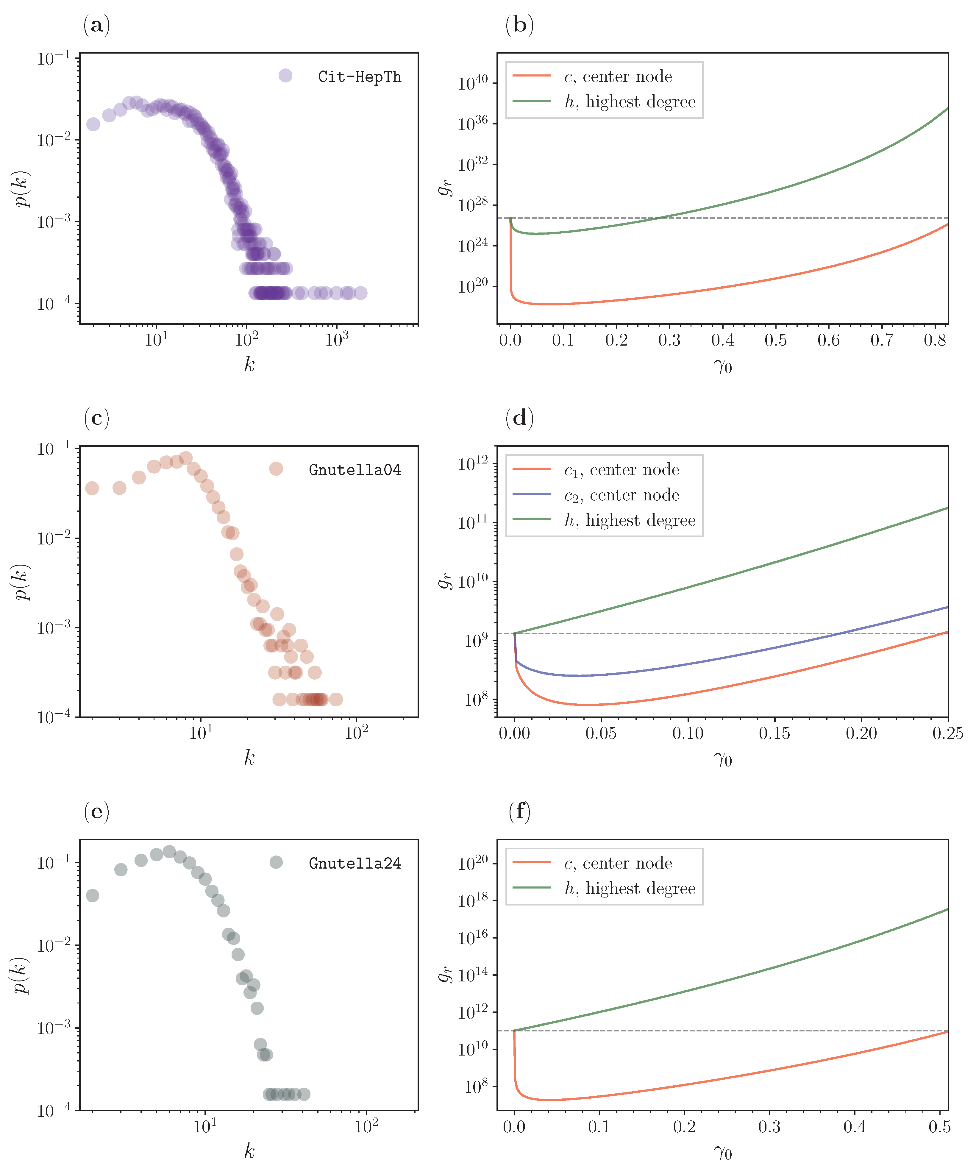
- Leskovec, J.; Krevl, A. SNAP Datasets: Stanford Large Network Dataset Collection. 2014. Available online: http://snap.stanford.edu/data (accessed on 1 September 2022).
- Leskovec, J.; Kleinberg, J.; Faloutsos, C. Graphs over time: Densification laws, shrinking diameters and possible explanations. In Proceedings of the Eleventh ACM SIGKDD International Conference on Knowledge Discovery in Data Mining, Chicago, IL, USA, 21–24 August 2005; pp. 177–187. [Google Scholar]
- Ripeanu, M.; Foster, I.; Iamnitchi, A. Mapping the gnutella network: Properties of large-scale peer-to-peer systems and implications for system design. arXiv 2002, arXiv:cs/0209028. [Google Scholar]
- Leskovec, J.; Kleinberg, J.; Faloutsos, C. Graph evolution: Densification and shrinking diameters. ACM Trans. Knowl. Discov. Data (TKDD) 2007, 1, 2–es. [Google Scholar] [CrossRef]
- Clauset, A.; Shalizi, C.R.; Newman, M.E. Power-law distributions in empirical data. SIAM Rev. 2009, 51, 661–703. [Google Scholar] [CrossRef]
- Broido, A.D.; Clauset, A. Scale-free networks are rare. Nat. Commun. 2019, 10, 1017. [Google Scholar] [CrossRef]
- Goh, K.I.; Oh, E.; Jeong, H.; Kahng, B.; Kim, D. Classification of scale-free networks. Proc. Natl. Acad. Sci. USA 2002, 99, 12583–12588. [Google Scholar] [CrossRef] [PubMed]
- Sarkar, M.; Gupta, S. Biased random walk on random networks in presence of stochastic resetting: Exact results. J. Phys. A Math. Theor. 2022, 55, 42LT01. [Google Scholar] [CrossRef]
- Sinatra, R.; Gómez-Gardenes, J.; Lambiotte, R.; Nicosia, V.; Latora, V. Maximal-entropy random walks in complex networks with limited information. Phys. Rev. E 2011, 83, 030103. [Google Scholar] [CrossRef] [PubMed]
- Godec, A.; Metzler, R. Universal proximity effect in target search kinetics in the few-encounter limit. Phy. Rev. X 2016, 6, 041037. [Google Scholar] [CrossRef]
- Grebenkov, D.S.; Metzler, R.; Oshanin, G. Strong defocusing of molecular reaction times results from an interplay of geometry and reaction control. Commun. Chem. 2018, 1, 96. [Google Scholar] [CrossRef] [Green Version]


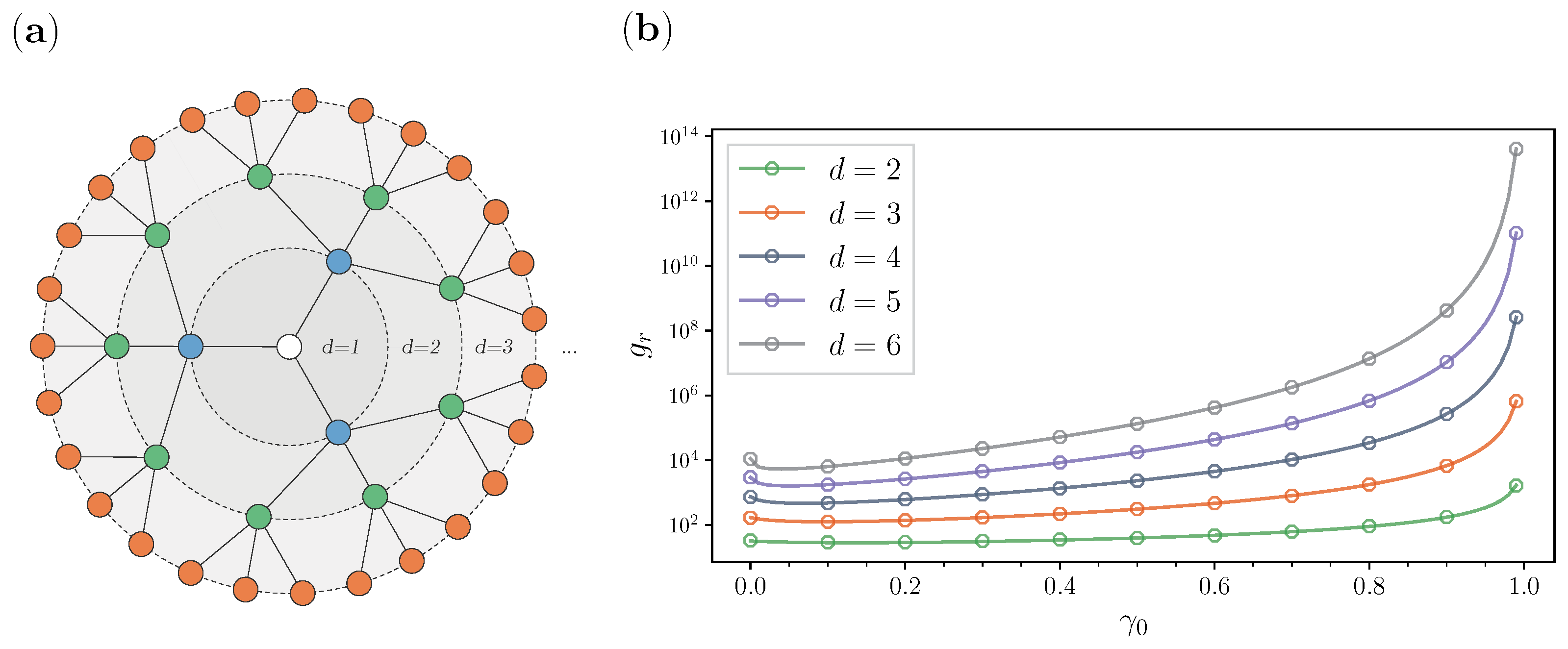
| d, Depth | N, No. Nodes | , Diameter | Improvement 1 |
|---|---|---|---|
| 2 | 13 | 4 | 11.1% |
| 3 | 40 | 6 | 25.4% |
| 4 | 121 | 8 | 36.7% |
| 5 | 364 | 10 | 45.2% |
| 6 | 1093 | 12 | 51.7% |
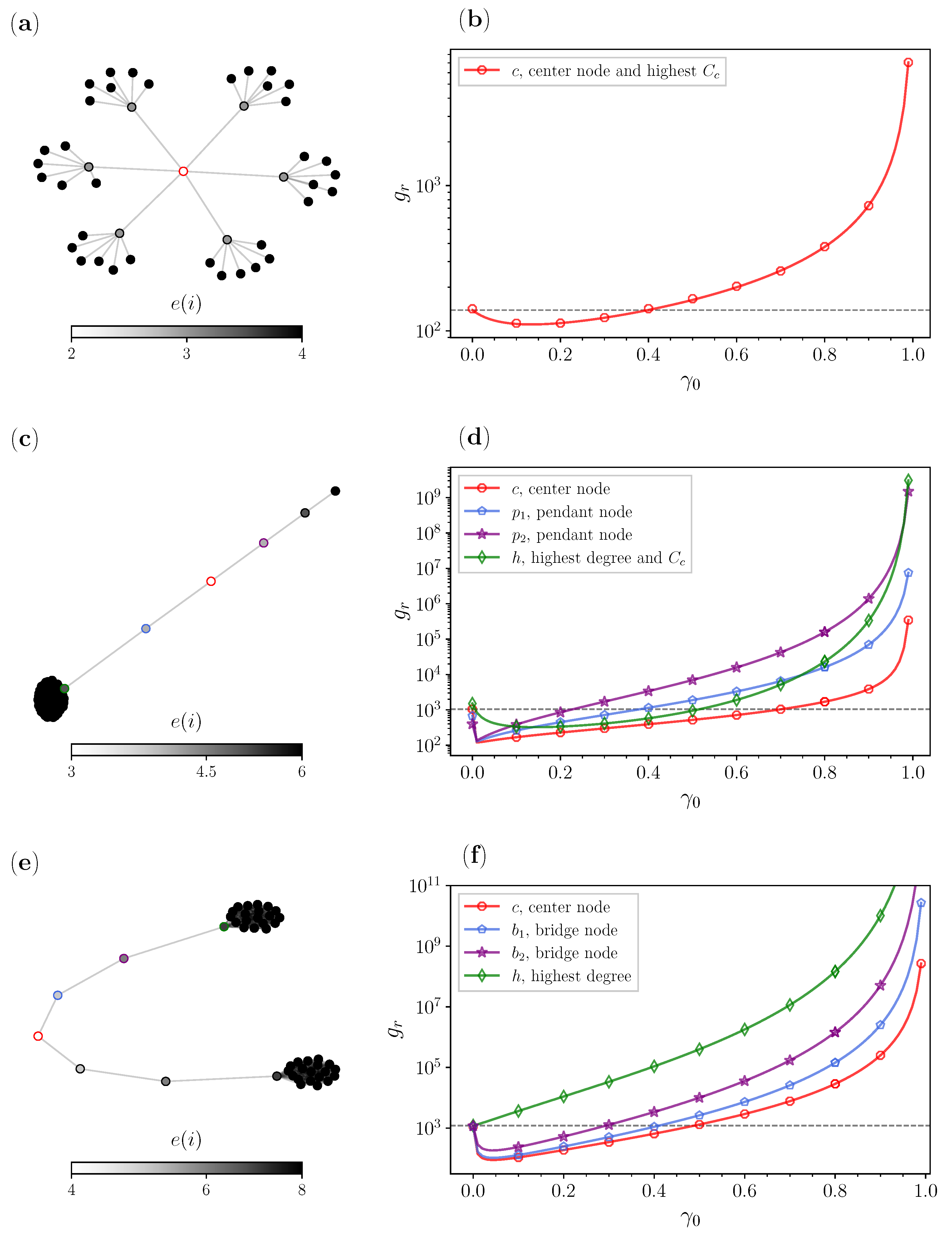
| Type of Special Graph | Resetting Node Candidate | Improvement 1 |
|---|---|---|
| Balanced tree | c, center/highest | 20.27% |
| Lollipop | c, center node | 88.49% |
| , pendant node | 81.14% | |
| , pendant node | 65.68% | |
| h, highest degree/ | 78.53% | |
| Barbell | c, center | 92.19% |
| , bridge node | 90.88% | |
| , bridge node | 84.30% | |
| h, highest degree | 0.00% |
Disclaimer/Publisher’s Note: The statements, opinions and data contained in all publications are solely those of the individual author(s) and contributor(s) and not of MDPI and/or the editor(s). MDPI and/or the editor(s) disclaim responsibility for any injury to people or property resulting from any ideas, methods, instructions or products referred to in the content. |
© 2023 by the authors. Licensee MDPI, Basel, Switzerland. This article is an open access article distributed under the terms and conditions of the Creative Commons Attribution (CC BY) license (https://creativecommons.org/licenses/by/4.0/).
Share and Cite
Zelenkovski, K.; Sandev, T.; Metzler, R.; Kocarev, L.; Basnarkov, L. Random Walks on Networks with Centrality-Based Stochastic Resetting. Entropy 2023, 25, 293. https://doi.org/10.3390/e25020293
Zelenkovski K, Sandev T, Metzler R, Kocarev L, Basnarkov L. Random Walks on Networks with Centrality-Based Stochastic Resetting. Entropy. 2023; 25(2):293. https://doi.org/10.3390/e25020293
Chicago/Turabian StyleZelenkovski, Kiril, Trifce Sandev, Ralf Metzler, Ljupco Kocarev, and Lasko Basnarkov. 2023. "Random Walks on Networks with Centrality-Based Stochastic Resetting" Entropy 25, no. 2: 293. https://doi.org/10.3390/e25020293