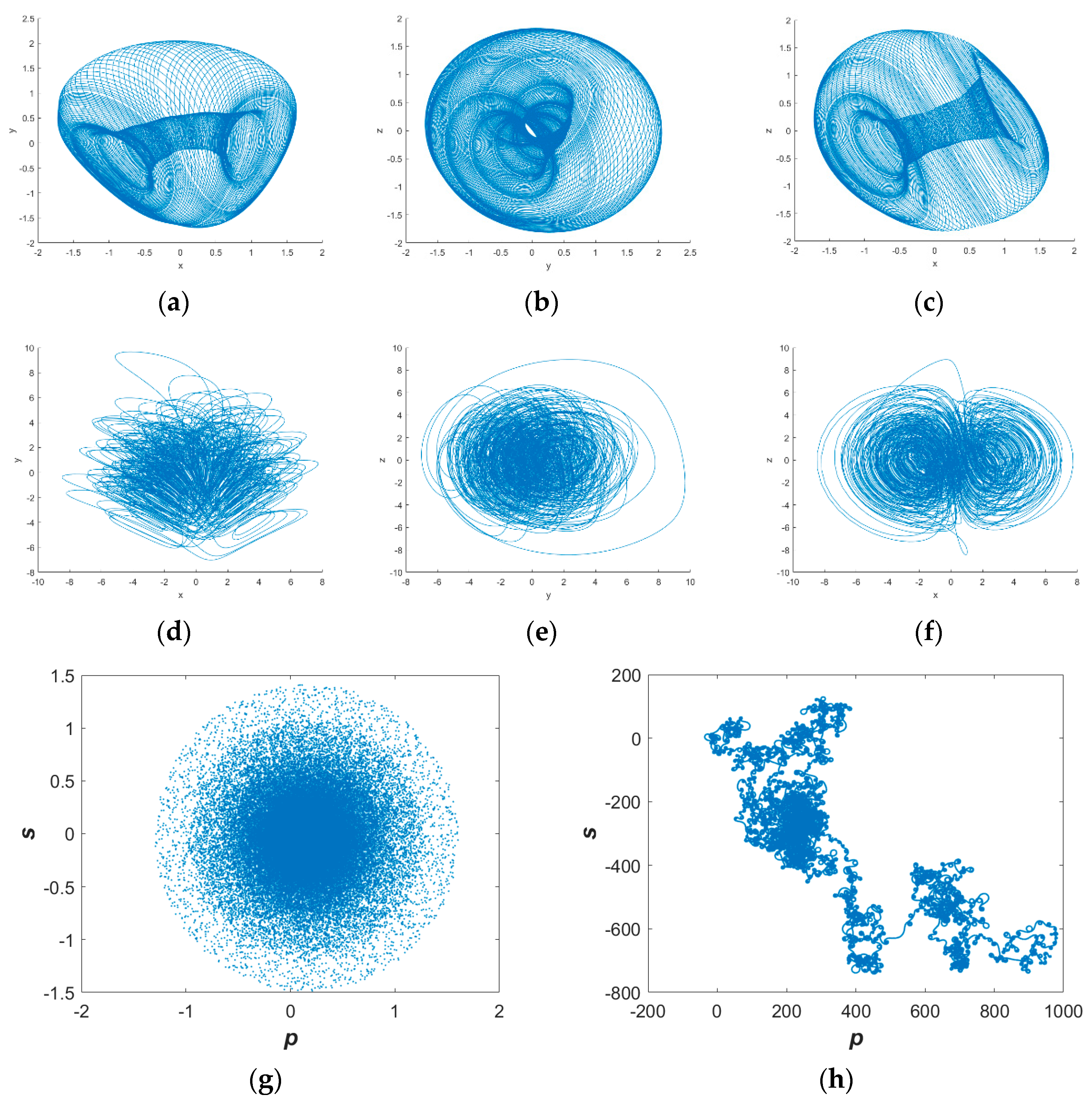
Figure 1.
Basic phase diagram of the system: (a) x–y Plane (period); (b) y–z Plane (period); (c) x–z Plane (period); (d) x–y Plane (Chaos); (e) y–z Plane (Chaos); (f) x–z Plane (Chaos); (g) 0–1 test (periodic); (h) 0–1 test (chaotic).
Figure 1.
Basic phase diagram of the system: (a) x–y Plane (period); (b) y–z Plane (period); (c) x–z Plane (period); (d) x–y Plane (Chaos); (e) y–z Plane (Chaos); (f) x–z Plane (Chaos); (g) 0–1 test (periodic); (h) 0–1 test (chaotic).
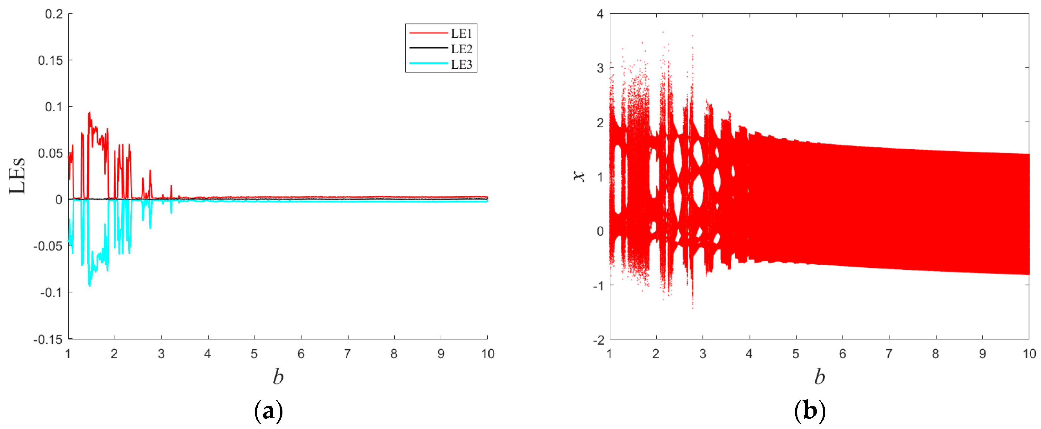
Figure 2.
Lyapunov exponential spectrum and bifurcation diagram with b: (a) Lyapunov exponential spectra; (b) bifurcation diagram.
Figure 2.
Lyapunov exponential spectrum and bifurcation diagram with b: (a) Lyapunov exponential spectra; (b) bifurcation diagram.
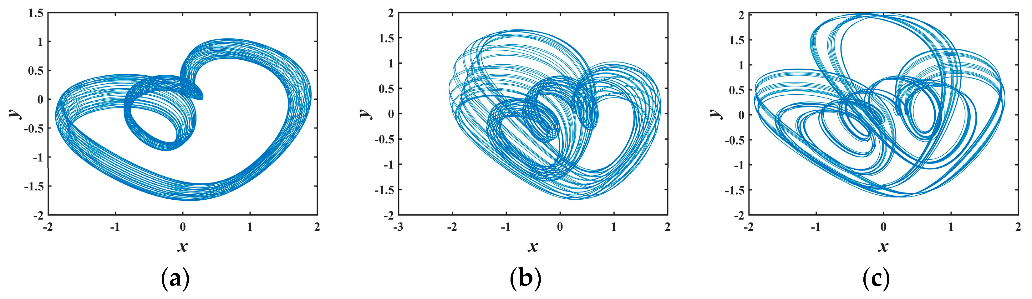
Figure 3.
Various phase diagrams varying with b: (a) b = 1.2; (b) b = 1.9; (c) b = 2.2; (d) b = 2.4; (e) b = 2.8; (f) b = 4.6.
Figure 3.
Various phase diagrams varying with b: (a) b = 1.2; (b) b = 1.9; (c) b = 2.2; (d) b = 2.4; (e) b = 2.8; (f) b = 4.6.
Figure 4.
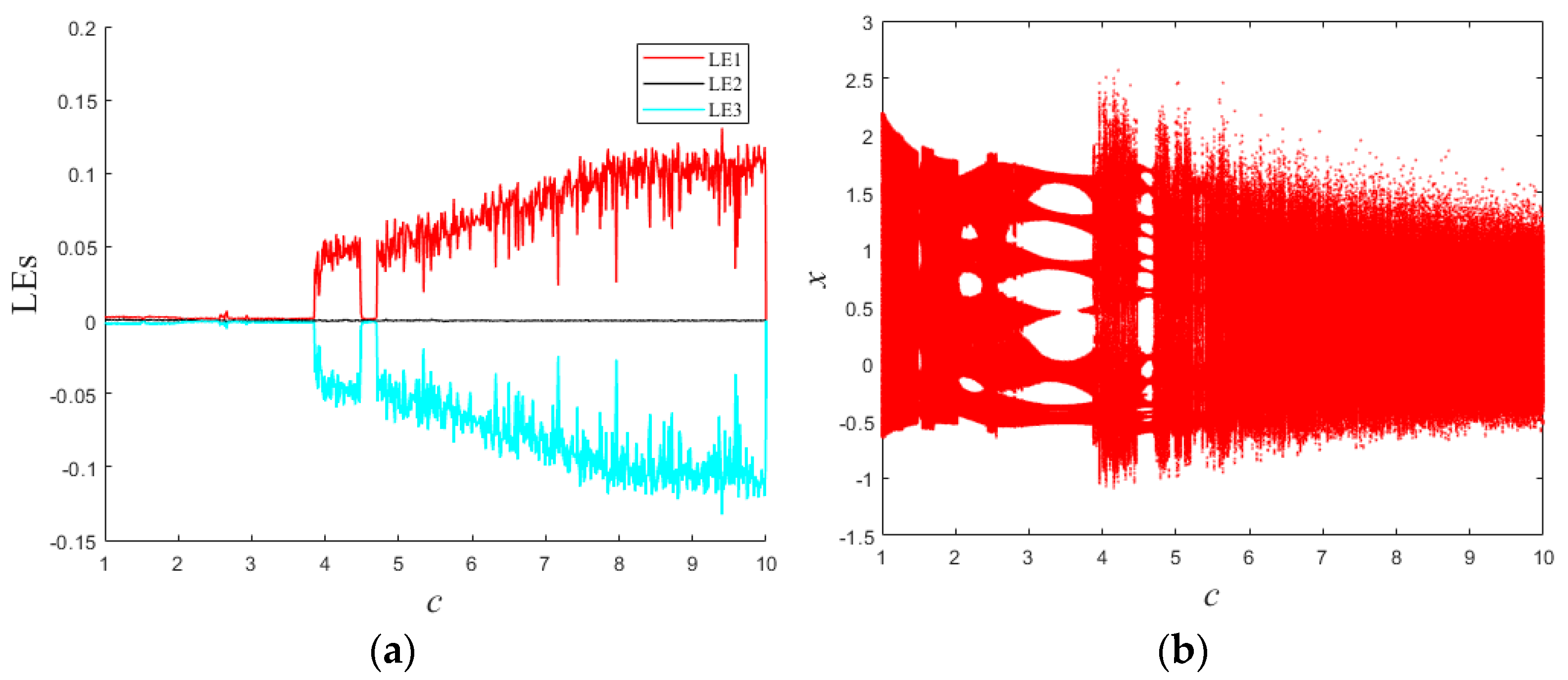
Lyapunov exponential spectrum and bifurcation diagram with c: (a) Lyapunov exponential spectrum; (b) bifurcation diagram.
Figure 4.
Lyapunov exponential spectrum and bifurcation diagram with c: (a) Lyapunov exponential spectrum; (b) bifurcation diagram.
Figure 5.
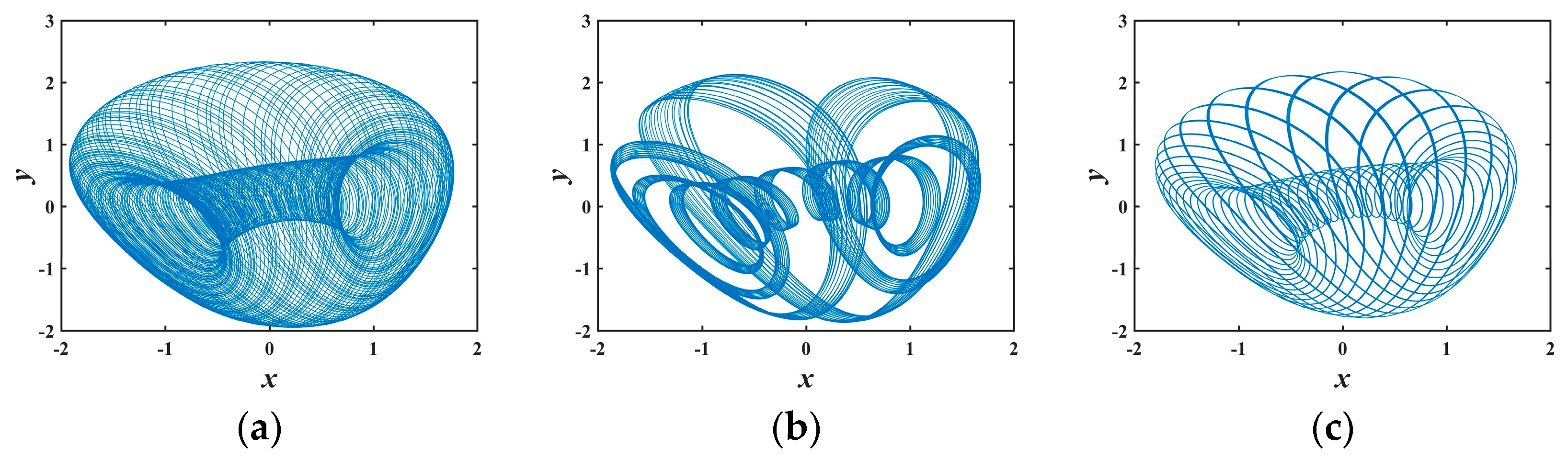
Various phase diagrams varying with c: (a) c = 1.4; (b) c = 1.5; (c) c = 1.7; (d) c = 3.3; (e) c = 4; (f) c = 8.5.
Figure 5.
Various phase diagrams varying with c: (a) c = 1.4; (b) c = 1.5; (c) c = 1.7; (d) c = 3.3; (e) c = 4; (f) c = 8.5.
Figure 6.
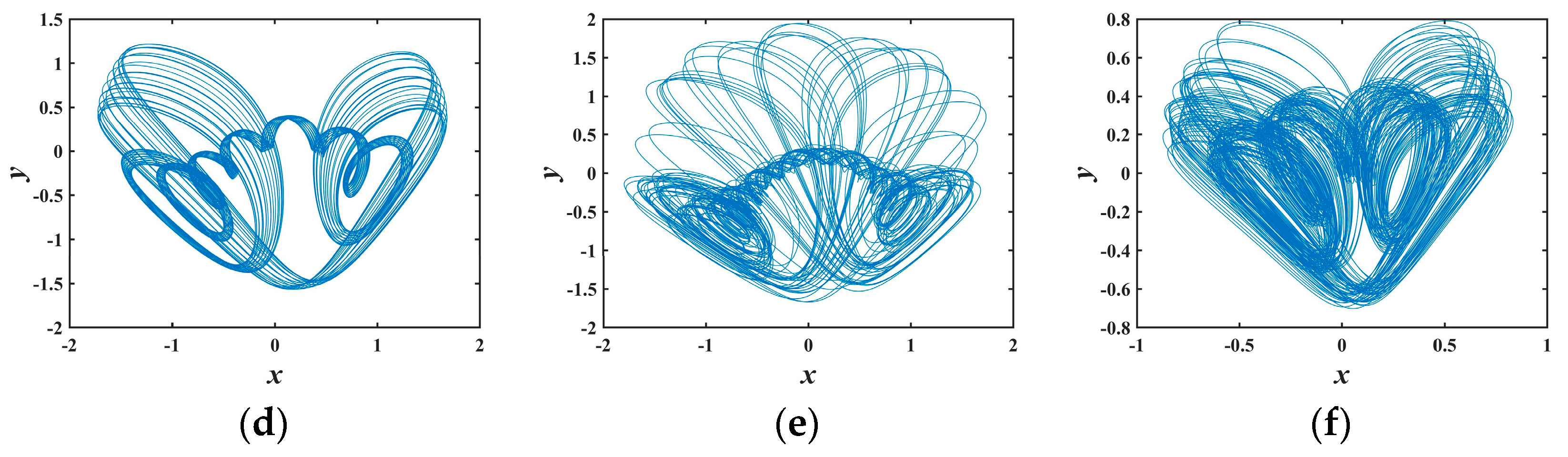
Lyapunov exponential spectra and bifurcation diagram with d: (a) Lyapunov exponential spectra; (b) bifurcation diagram.
Figure 6.
Lyapunov exponential spectra and bifurcation diagram with d: (a) Lyapunov exponential spectra; (b) bifurcation diagram.
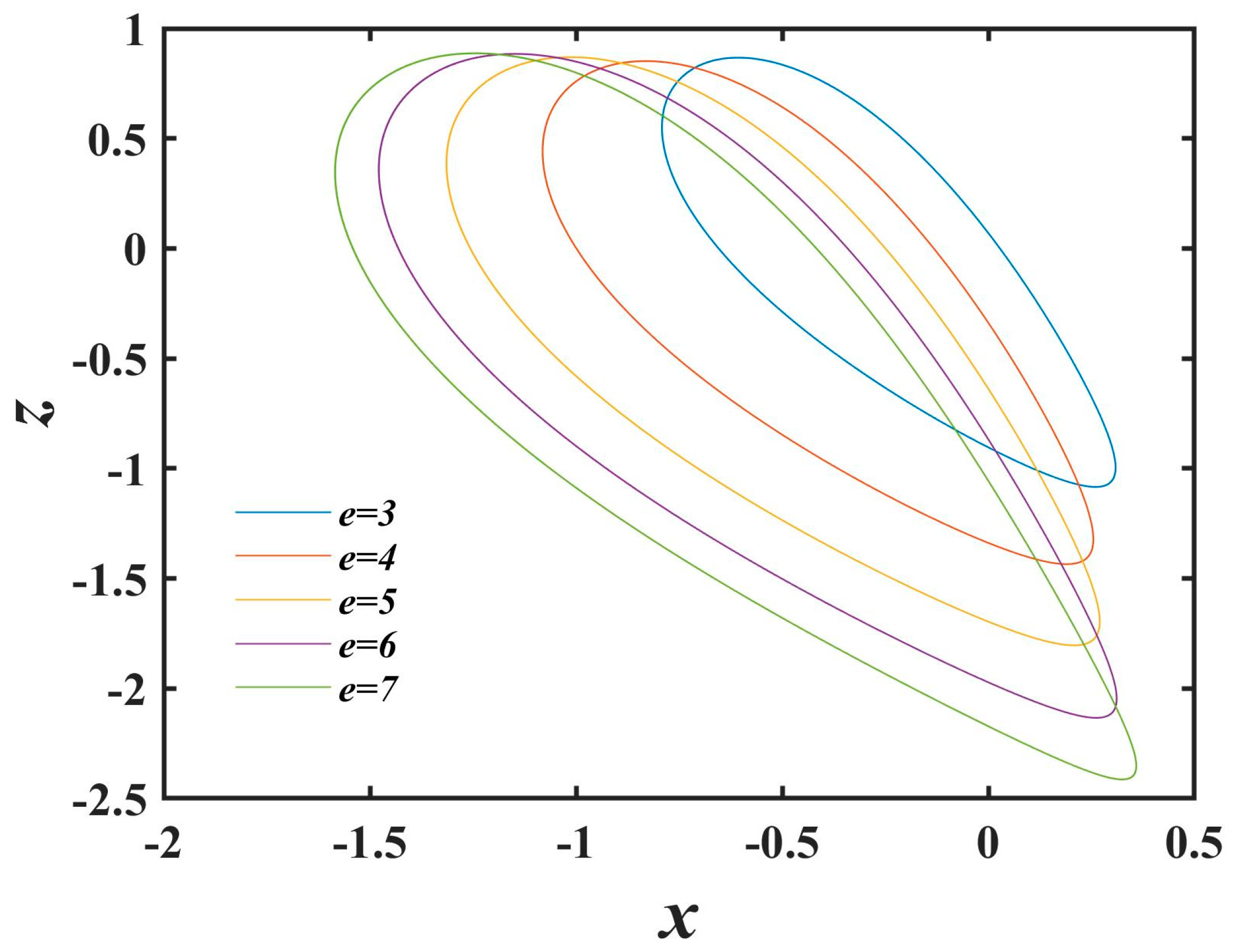
Figure 7.
Phase trajectories varying with e.
Figure 7.
Phase trajectories varying with e.
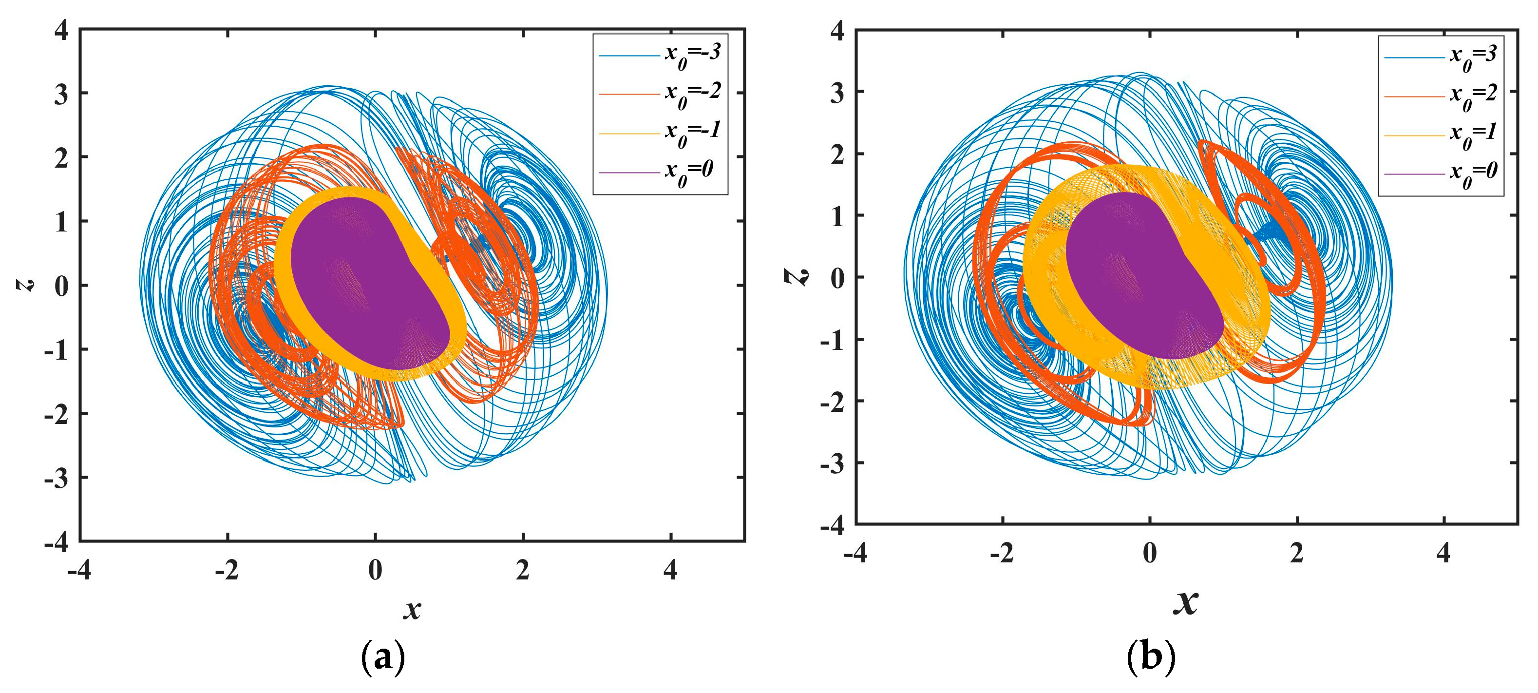
Figure 8.
Expansion and contraction behavior with x0: (a) contraction behavior; (b) expansion behavior.
Figure 8.
Expansion and contraction behavior with x0: (a) contraction behavior; (b) expansion behavior.
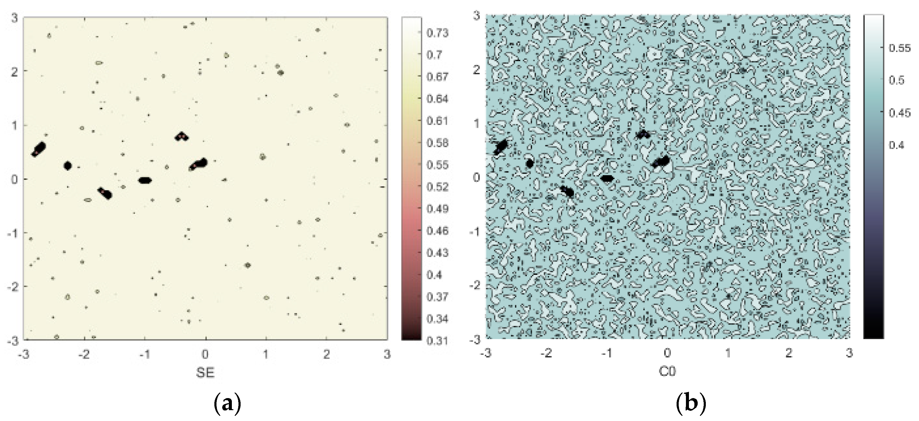
Figure 9.
SE and C0 complexity under condition a = 2; b = 4; c = 2; d = 10; e = 2; (a) SE (x0 ∈ [−3, 3], y0 ∈ [−3, 3]); (b) C0 (x0 ∈ [−3, 3], y0 ∈ [−3, 3]).
Figure 9.
SE and C0 complexity under condition a = 2; b = 4; c = 2; d = 10; e = 2; (a) SE (x0 ∈ [−3, 3], y0 ∈ [−3, 3]); (b) C0 (x0 ∈ [−3, 3], y0 ∈ [−3, 3]).
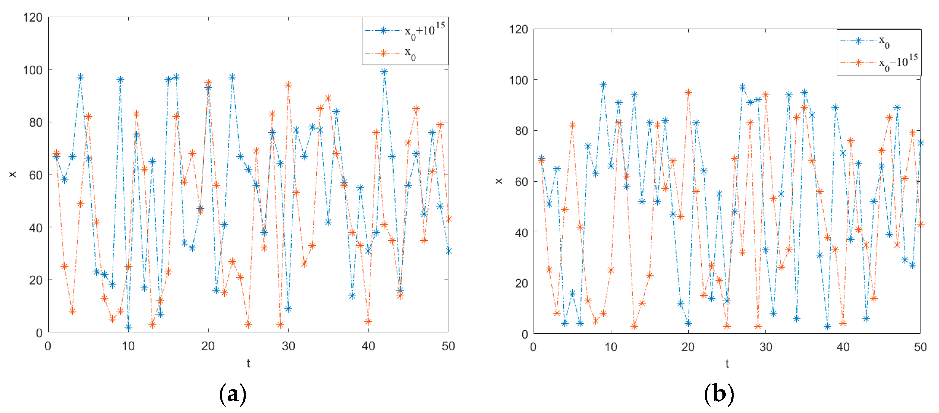
Figure 10.
Sensitivity test results for system (1). (a) x0 + 10−15; (b) x0 − 10−15.
Figure 10.
Sensitivity test results for system (1). (a) x0 + 10−15; (b) x0 − 10−15.
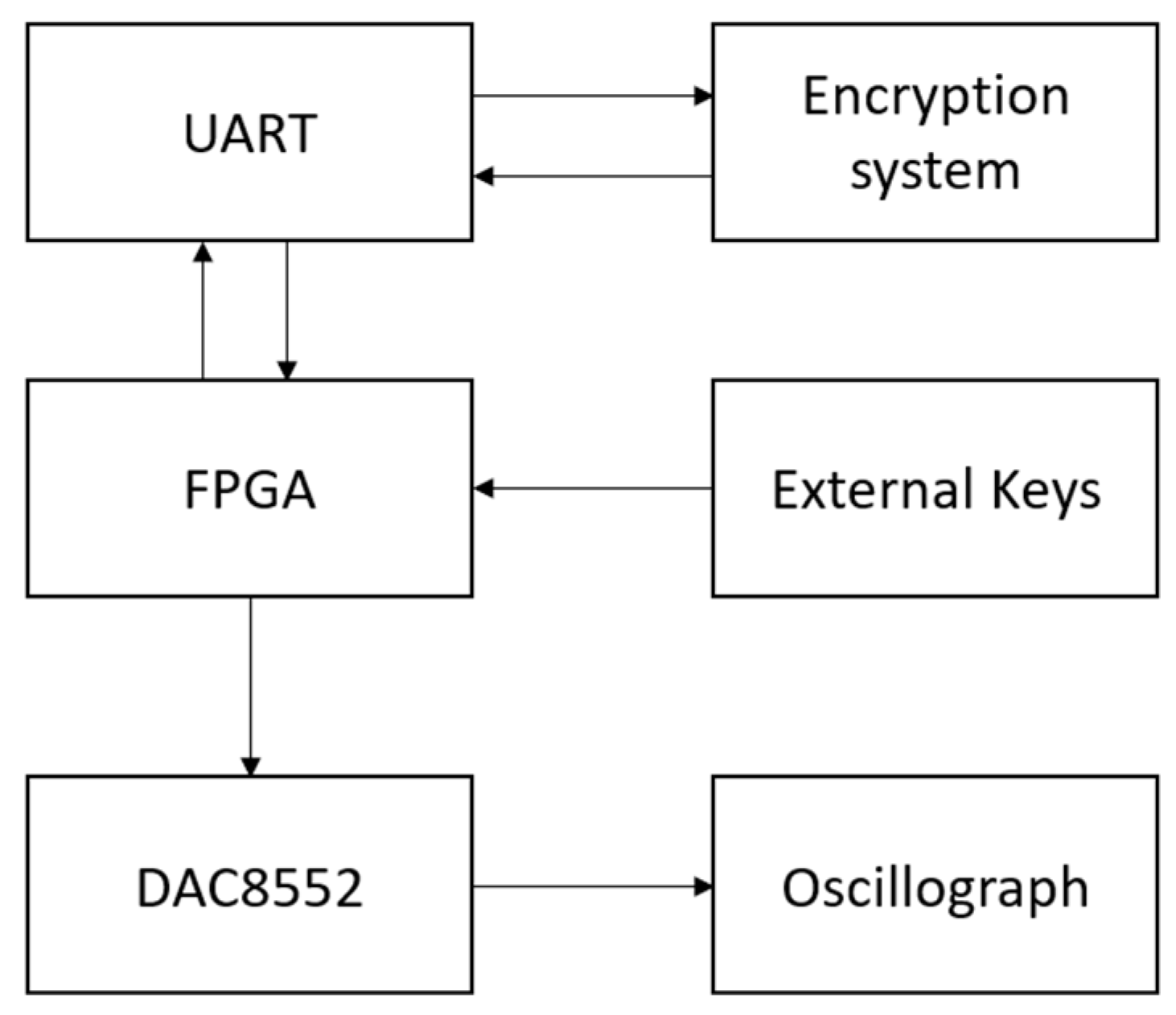
Figure 11.
Hardware platform design diagram.
Figure 11.
Hardware platform design diagram.
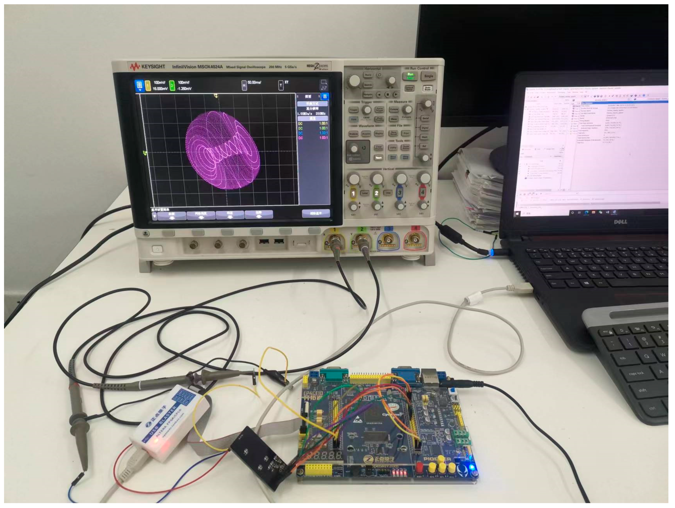
Figure 12.
Actual connection setup.
Figure 12.
Actual connection setup.
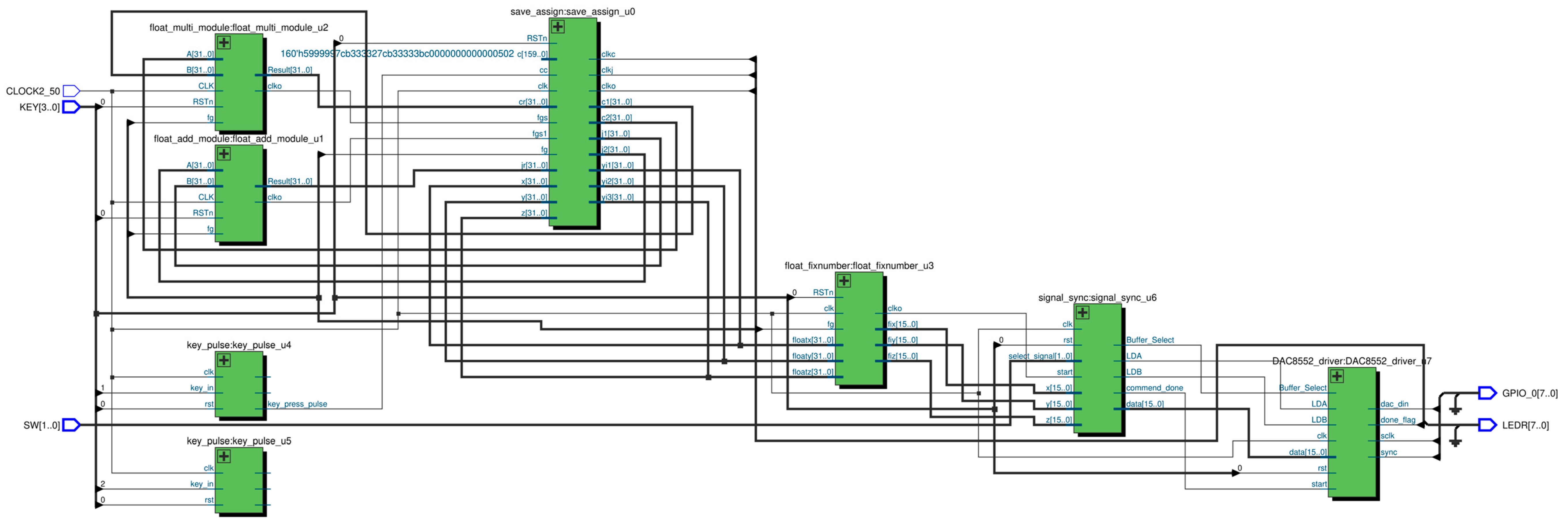
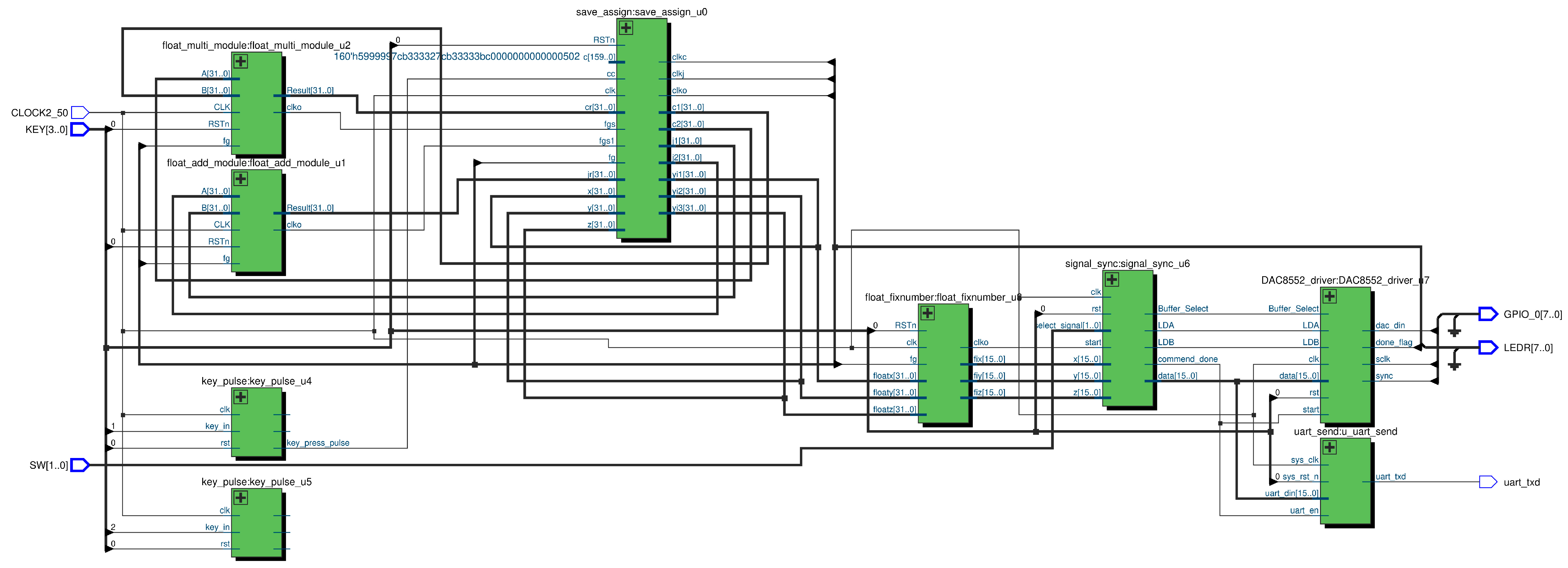
Figure 13.
Wiring diagram of the logic structure of the chaotic system.
Figure 13.
Wiring diagram of the logic structure of the chaotic system.
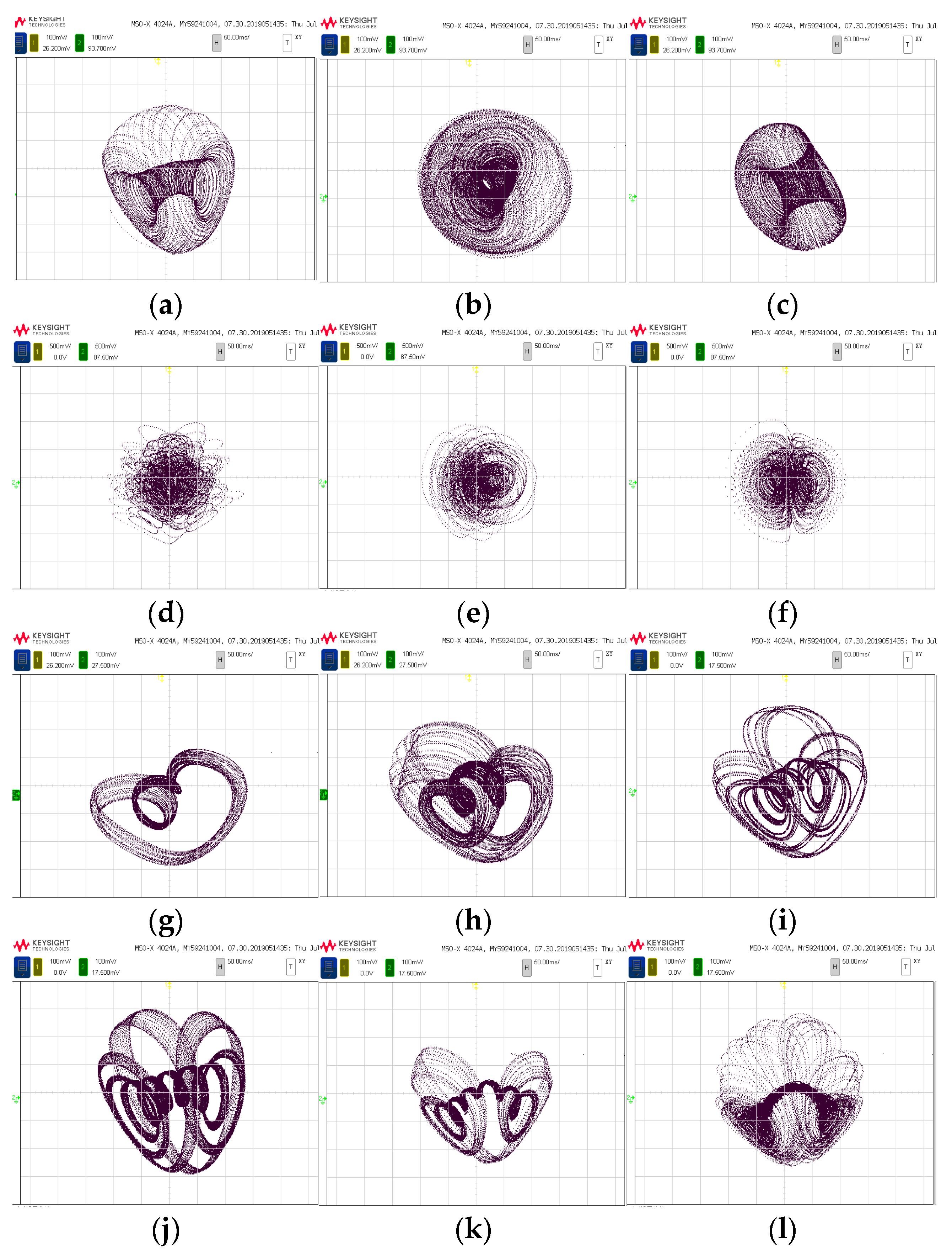
Figure 14.
FPGA realization of chaotic system attractor map; (a) x–y Plane (period); (b) y–z Plane (period); (c) x–z Plane (period); (d) x–y Plane (Chaos); (e) y–z Plane (Chaos); (f) x–z Plane (Chaos) (g) b = 1.2 (h) b = 1.9; (i) b = 2.2 (j) c = 1.5 (k) c = 3.3 (l) c = 4.
Figure 14.
FPGA realization of chaotic system attractor map; (a) x–y Plane (period); (b) y–z Plane (period); (c) x–z Plane (period); (d) x–y Plane (Chaos); (e) y–z Plane (Chaos); (f) x–z Plane (Chaos) (g) b = 1.2 (h) b = 1.9; (i) b = 2.2 (j) c = 1.5 (k) c = 3.3 (l) c = 4.
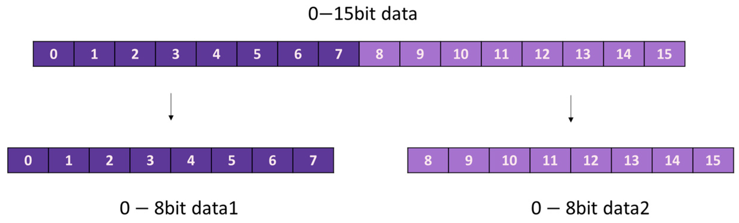
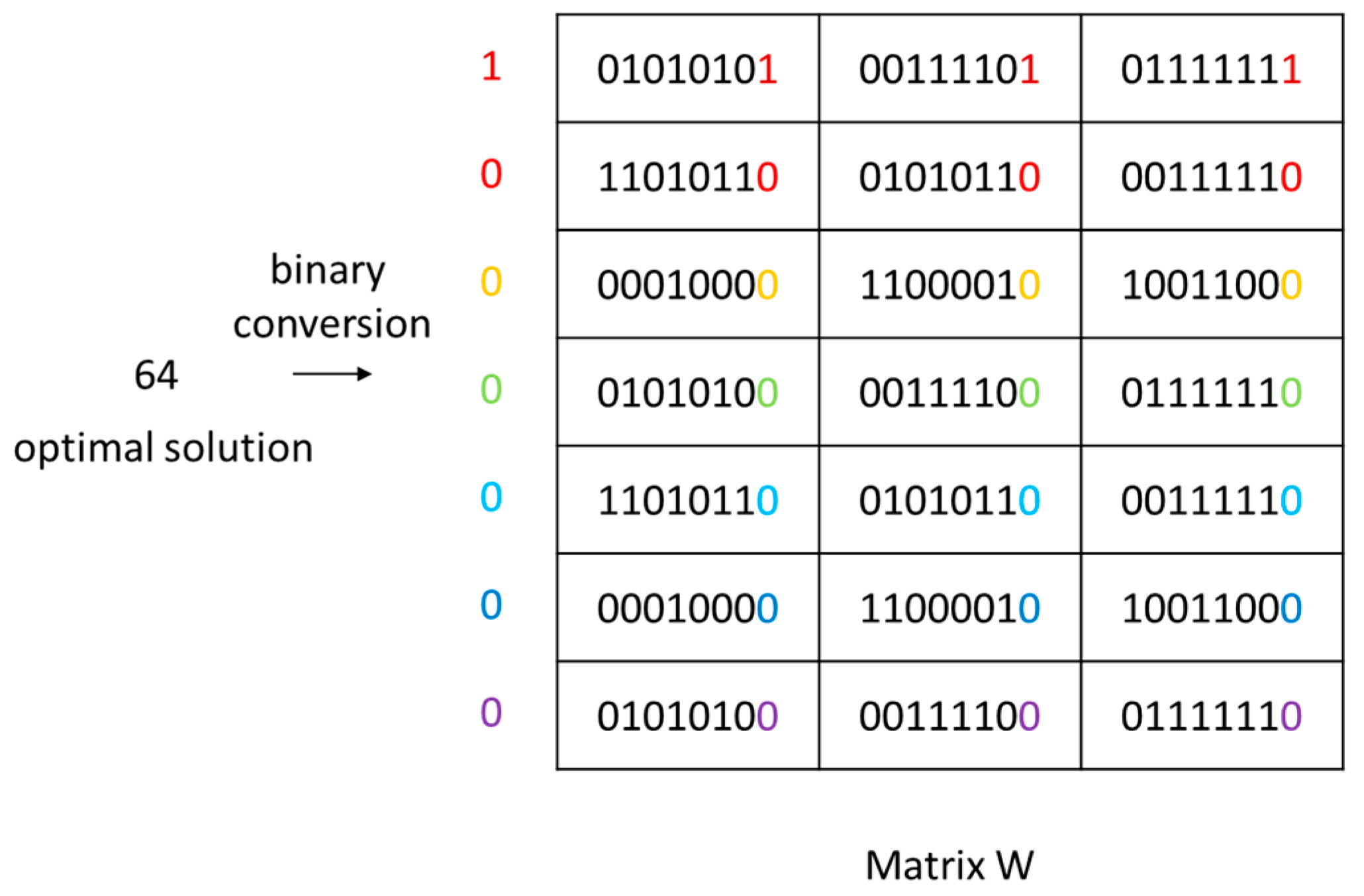
Figure 15.
Data decomposition schematic.
Figure 15.
Data decomposition schematic.
Figure 16.
Serial data receiving interface diagram.
Figure 16.
Serial data receiving interface diagram.
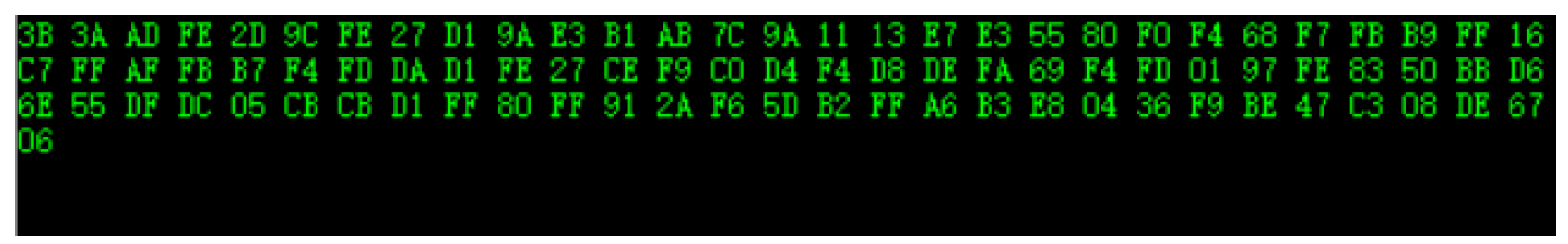
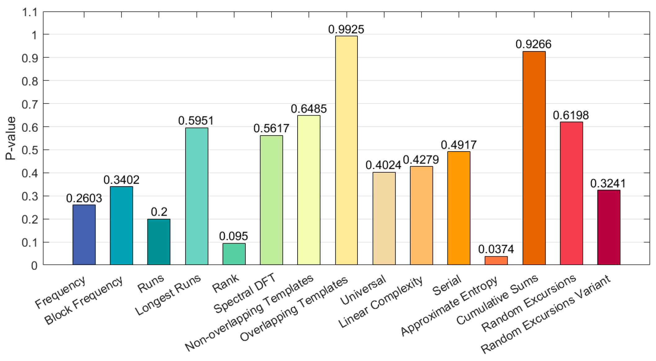
Figure 17.
NIST testing of serial data.
Figure 17.
NIST testing of serial data.
Figure 18.
Wiring diagram of the logical structure of the pseudo-random sequence generator.
Figure 18.
Wiring diagram of the logical structure of the pseudo-random sequence generator.
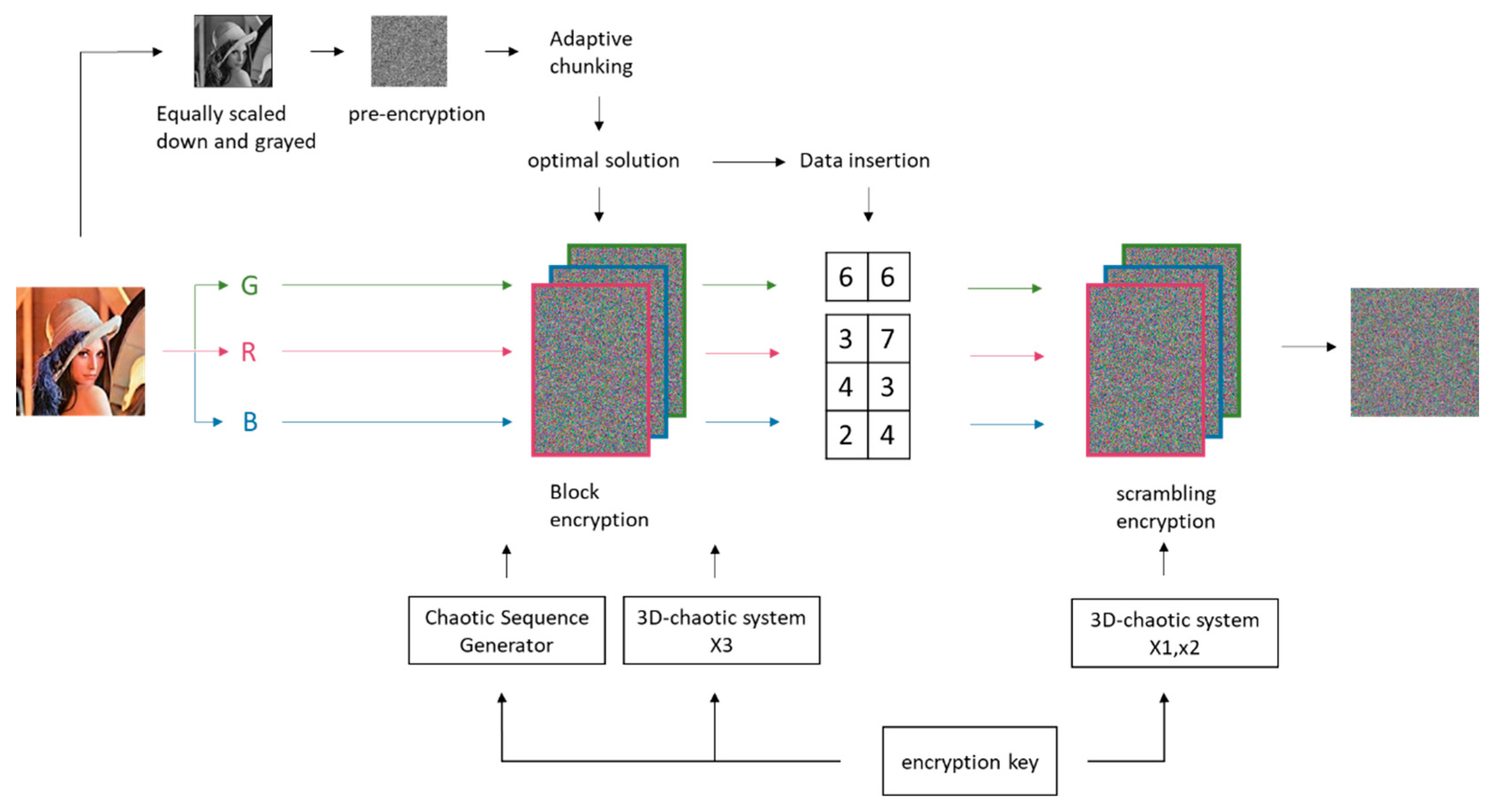
Figure 19.
encryption schematic.
Figure 19.
encryption schematic.
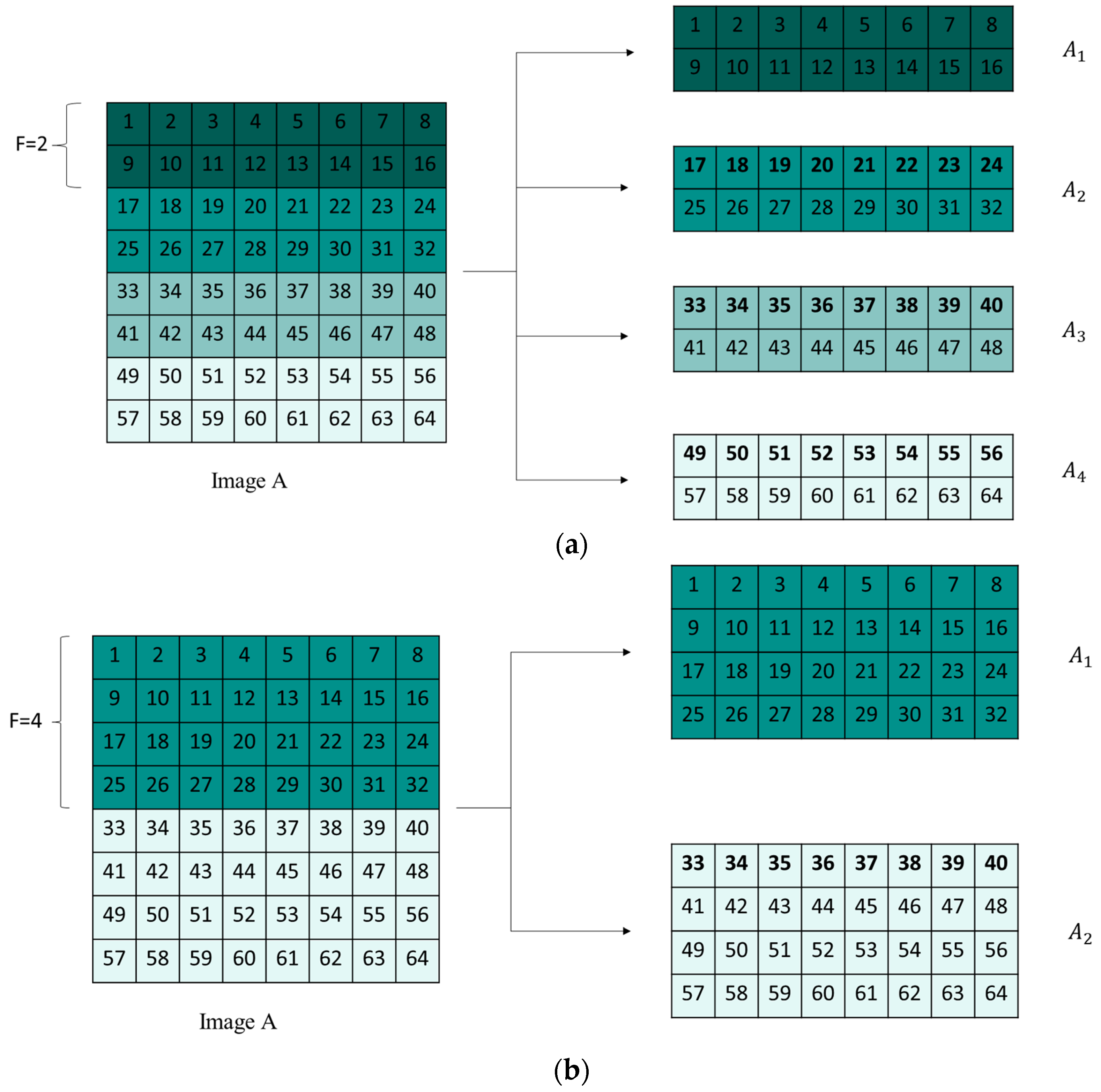
Figure 20.
Image chunk process: (a) F = 2; (b) F = 4.
Figure 20.
Image chunk process: (a) F = 2; (b) F = 4.
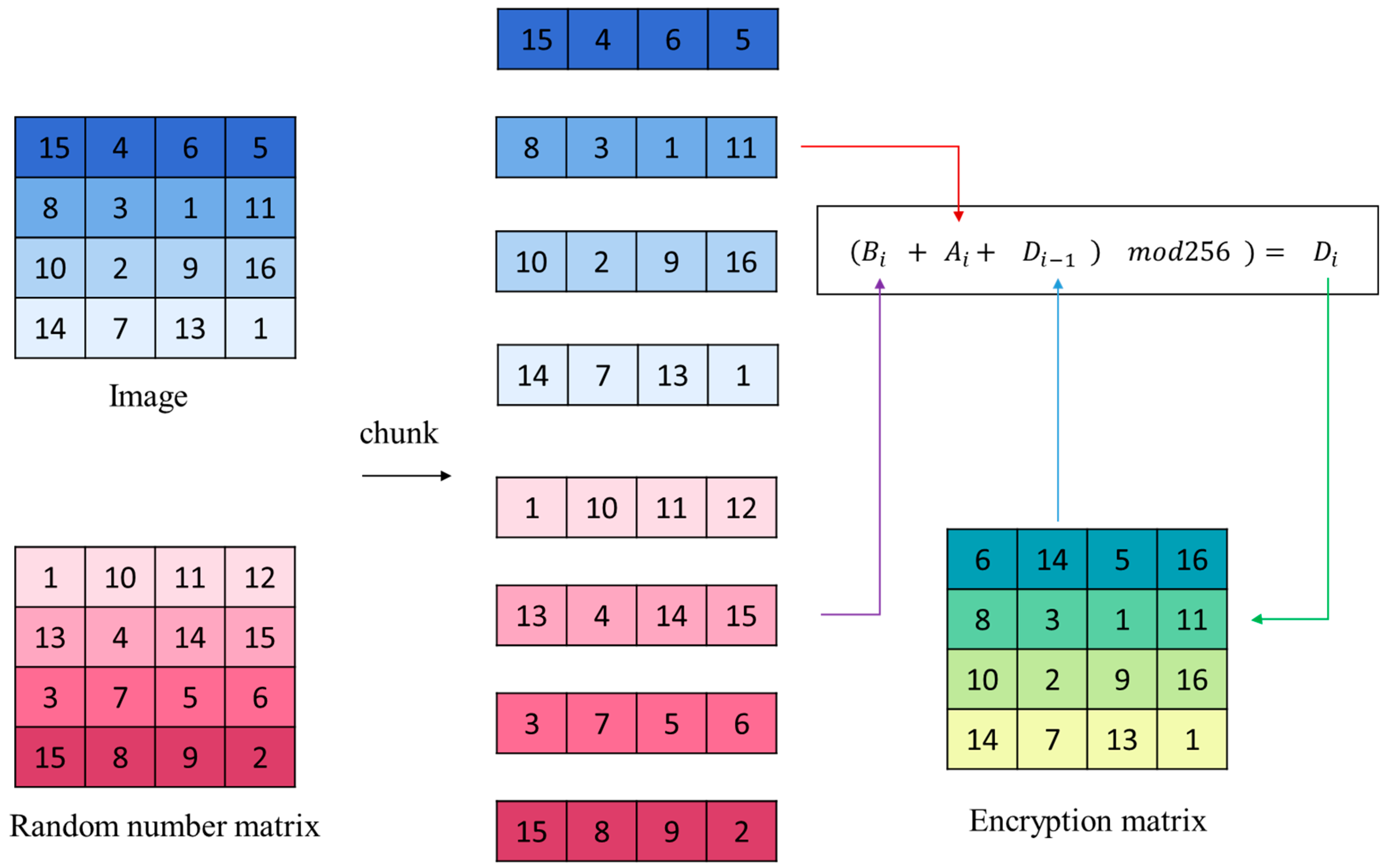
Figure 21.
Schematic diagram of chunk encryption.
Figure 21.
Schematic diagram of chunk encryption.
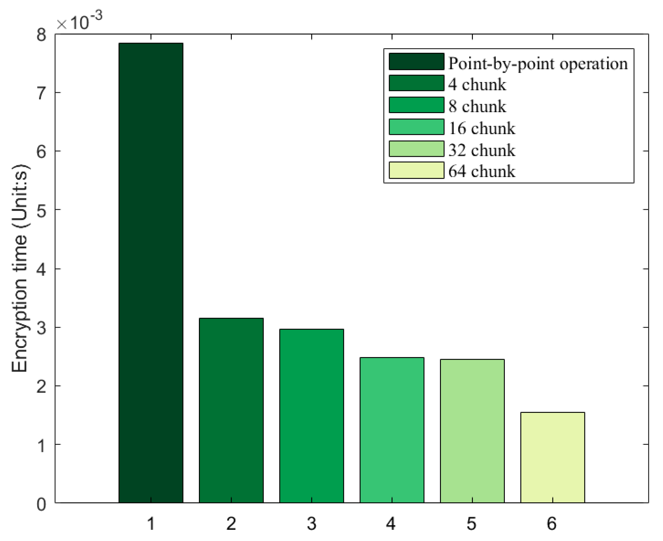
Figure 22.
Comparison of encryption times of different chunking policies (Unit: s).
Figure 22.
Comparison of encryption times of different chunking policies (Unit: s).
Figure 23.
Encryption performance of different images with different chunking strategies: (a) Baboon; (b) Barbara; (c); House (d) Pepper.
Figure 23.
Encryption performance of different images with different chunking strategies: (a) Baboon; (b) Barbara; (c); House (d) Pepper.
Figure 24.
Schematic diagram of data steganography.
Figure 24.
Schematic diagram of data steganography.
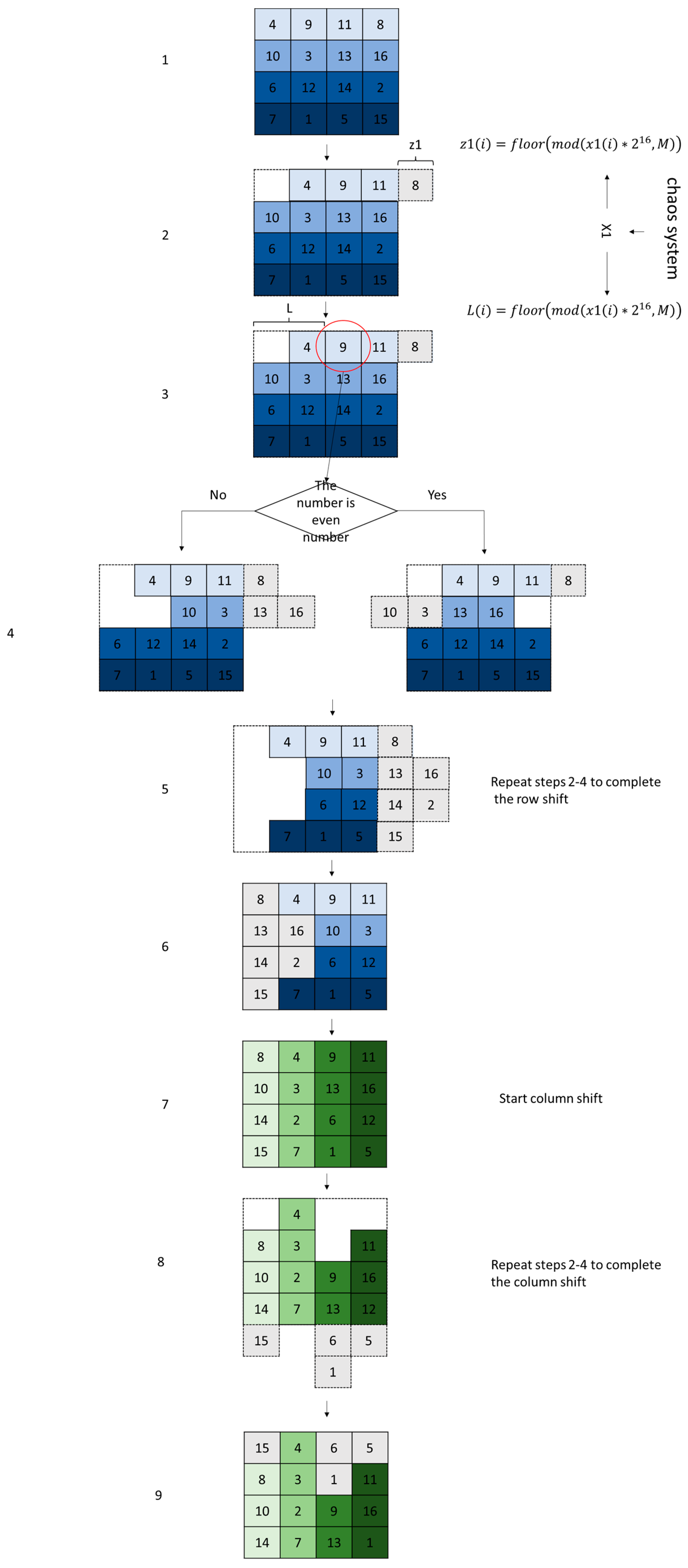
Figure 25.
Schematic diagram of disorganization.
Figure 25.
Schematic diagram of disorganization.
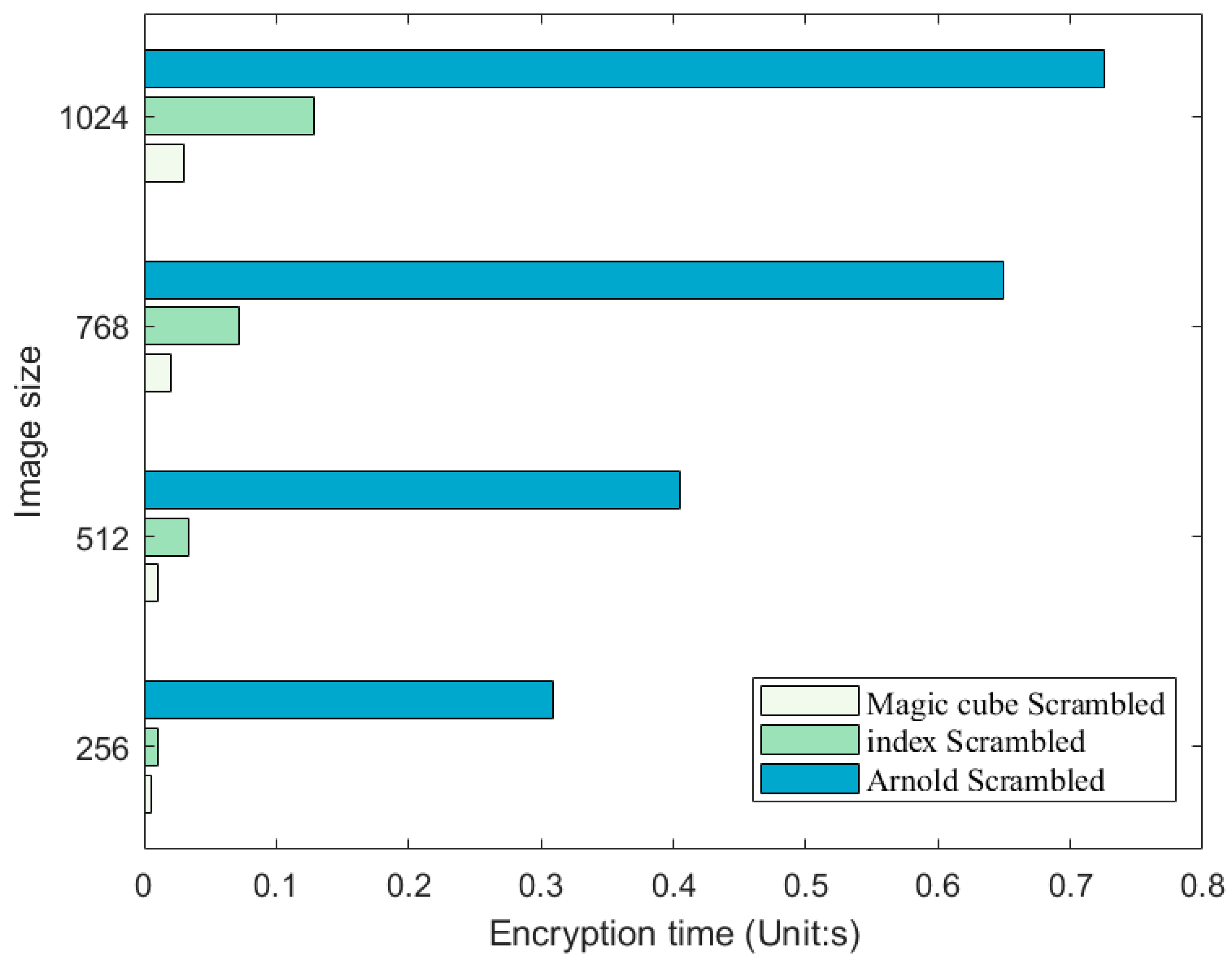
Figure 26.
Comparison of encryption times of different scrambling methods (Unit: s).
Figure 26.
Comparison of encryption times of different scrambling methods (Unit: s).
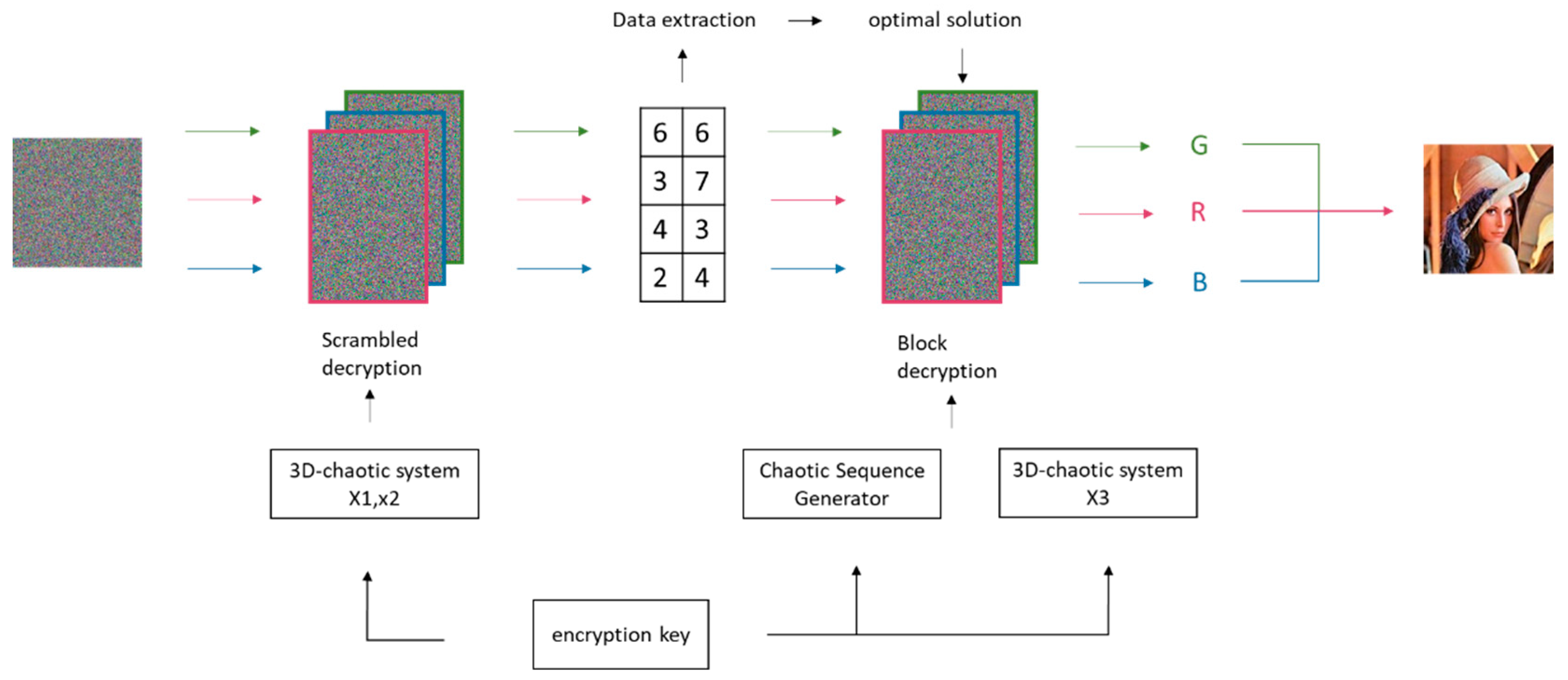
Figure 27.
Decryption schematic.
Figure 27.
Decryption schematic.
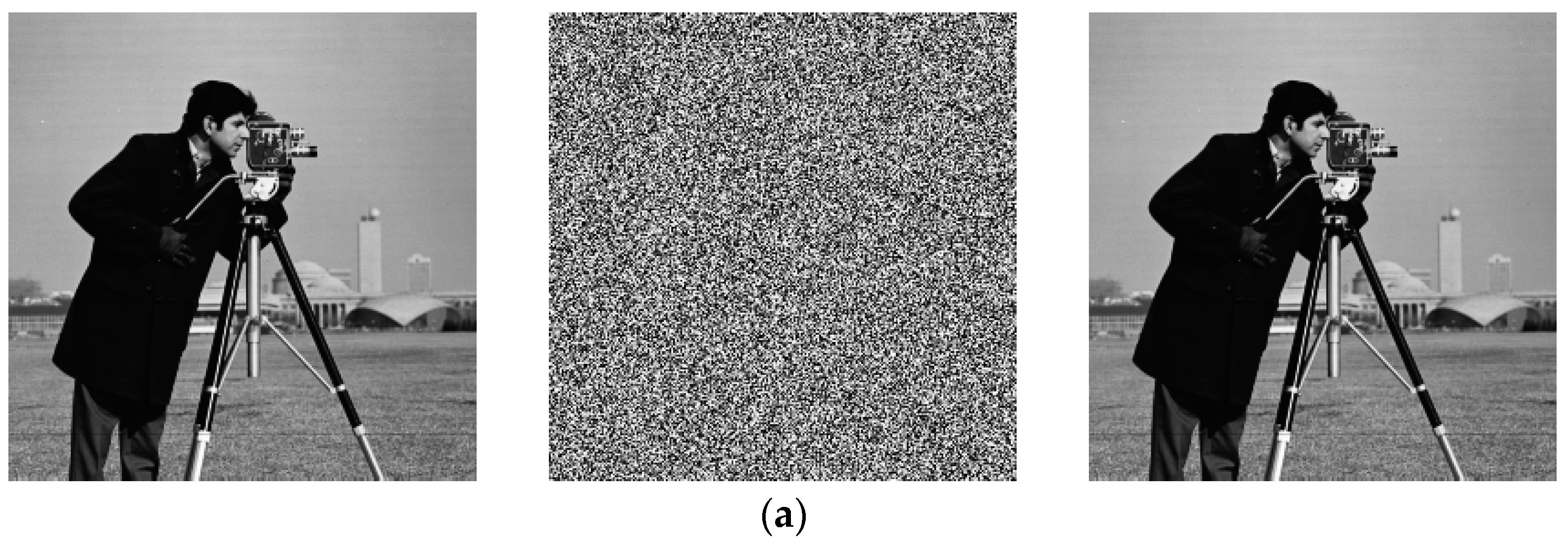
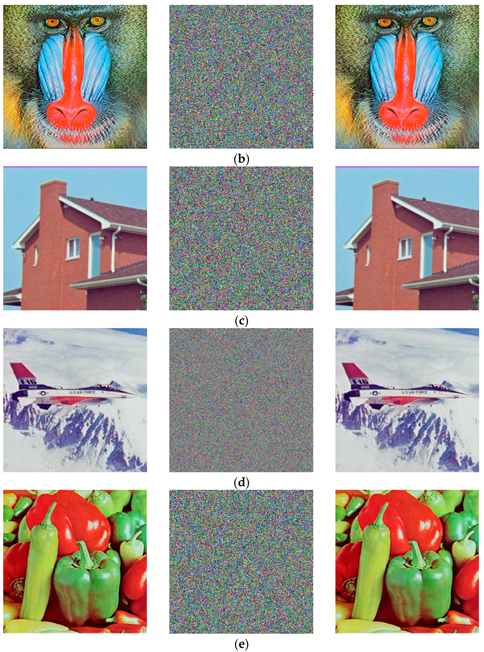
Figure 28.
Encryption and decryption renderings of the test images: (a) encryption and decryption image of cameraman; (b) encryption and decryption image of baboon; (c) encryption and decryption image of house; (d) encryption and decryption image of airplane (e) encryption and decryption image of pepper.
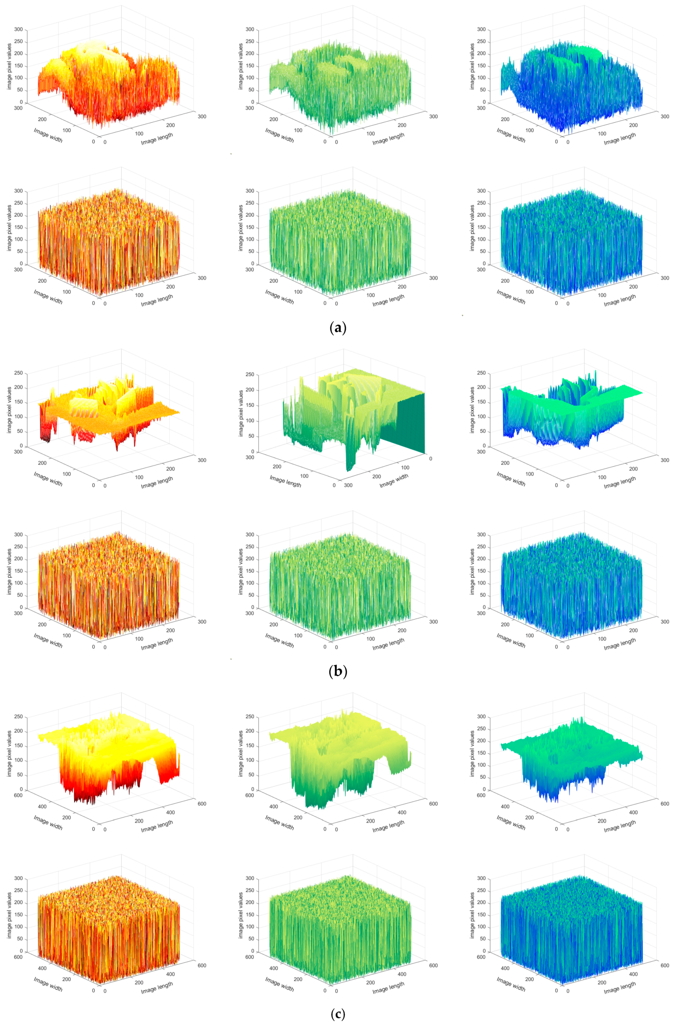
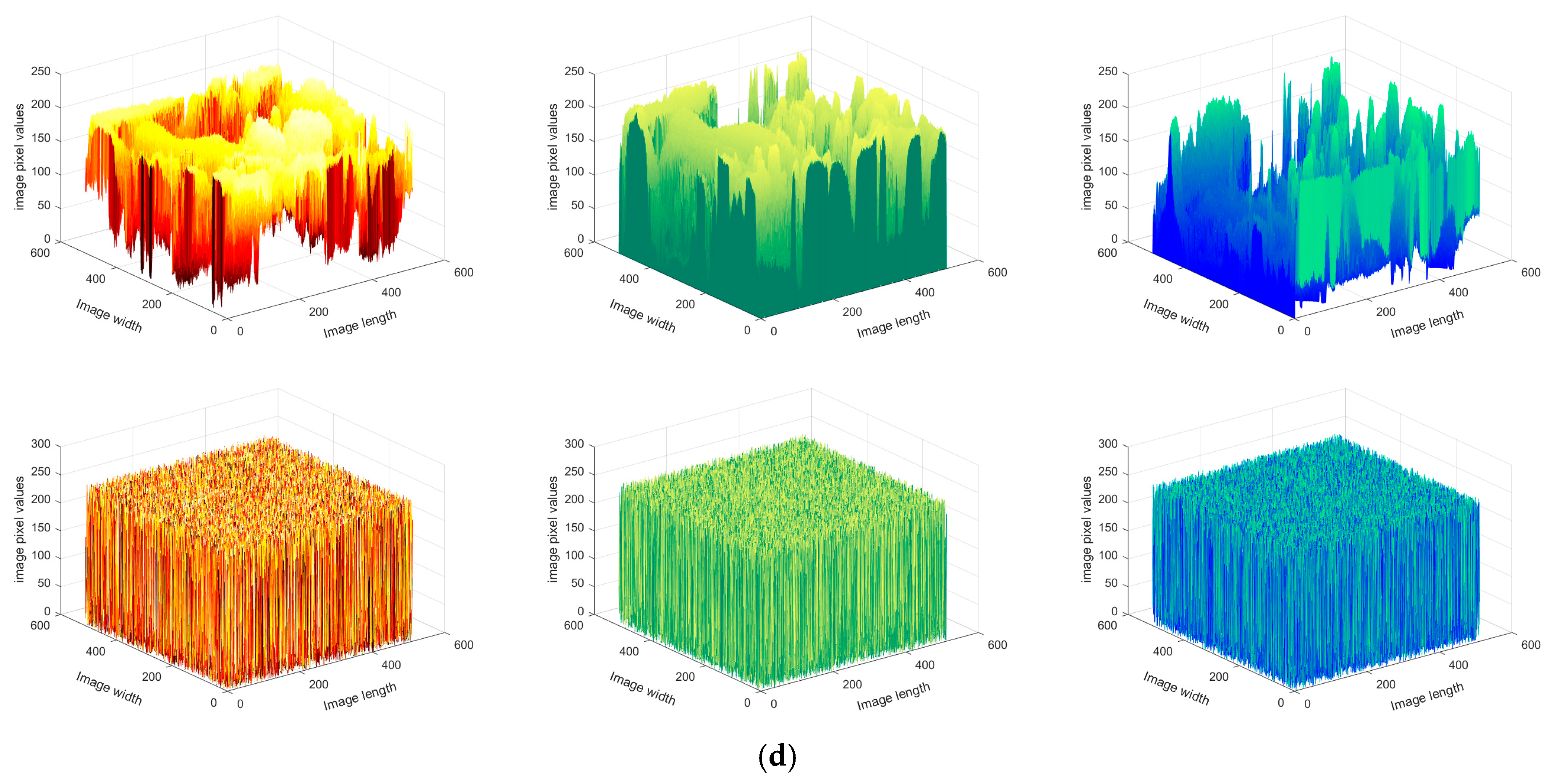
Figure 29.
Three-dimensional histograms of the original and encrypted images: (a) baboon, (b) house, (c) airplane, (d) pepper.
Figure 29.
Three-dimensional histograms of the original and encrypted images: (a) baboon, (b) house, (c) airplane, (d) pepper.
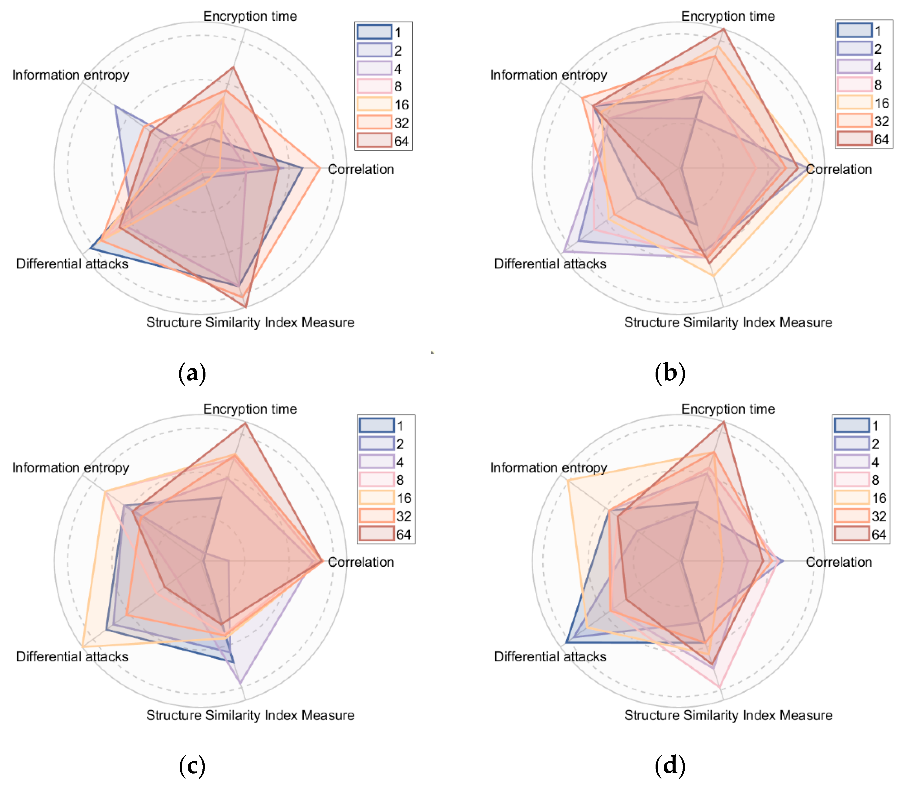
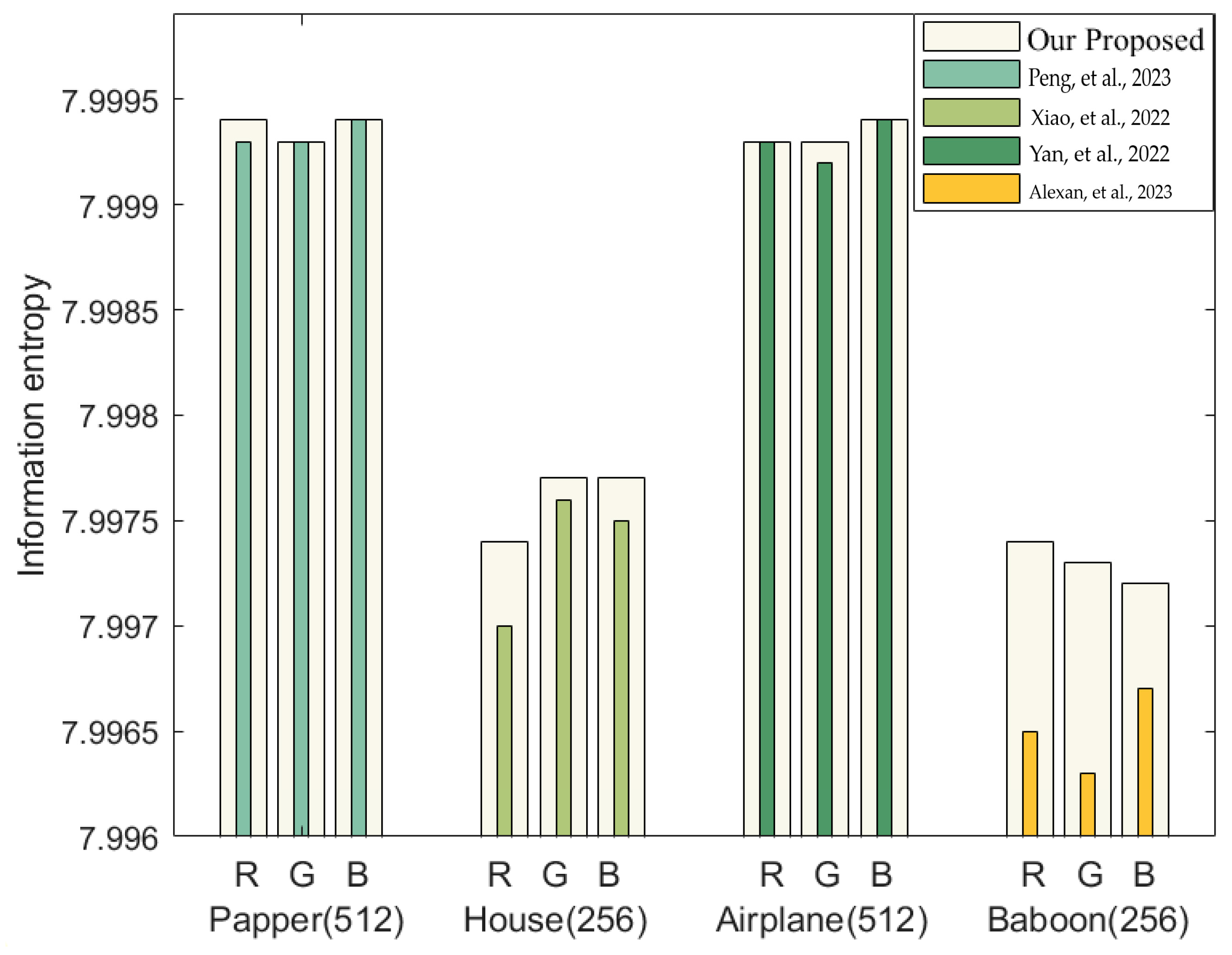
Figure 30.
Comparison of information entropy with other algorithms [
49,
50,
51,
52].
Figure 30.
Comparison of information entropy with other algorithms [
49,
50,
51,
52].
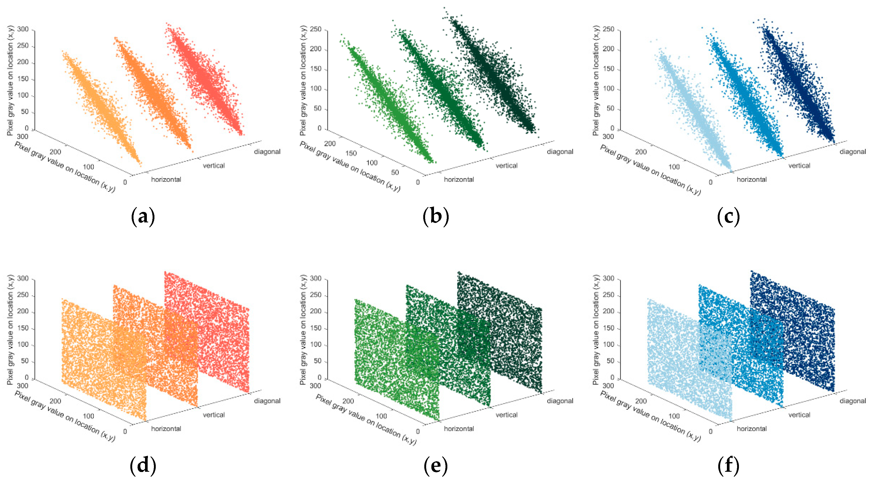
Figure 31.
Correlation comparison before and after image encryption. (a) R-channel correlation before encryption. (b) G-channel correlation before encryption. (c) B-channel correlation before encryption. (d) R-channel correlation after encryption (e) G-channel correlation after encryption. (f) B-channel correlation after encryption.
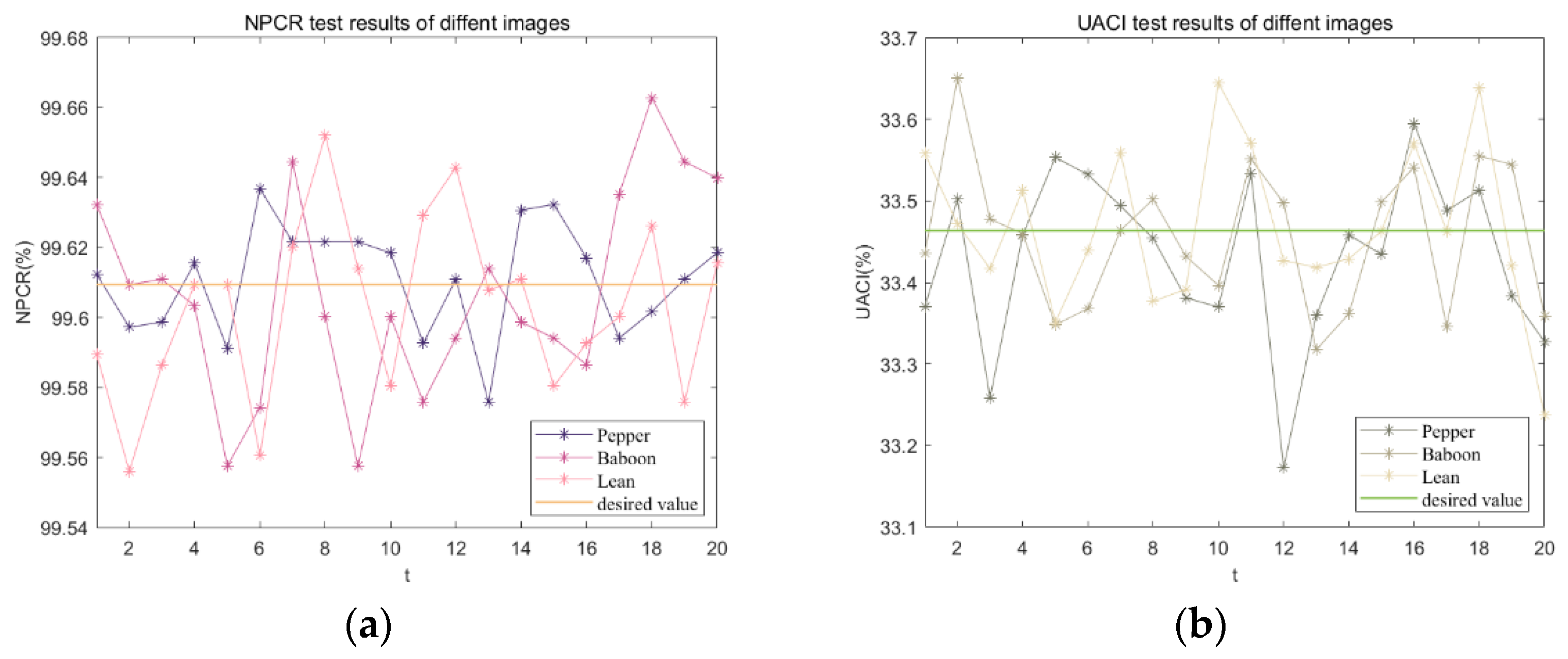
Figure 32.
Anti-differential attack test: (a) NPCR test results for different images; (b) UACI test results for different images.
Figure 32.
Anti-differential attack test: (a) NPCR test results for different images; (b) UACI test results for different images.
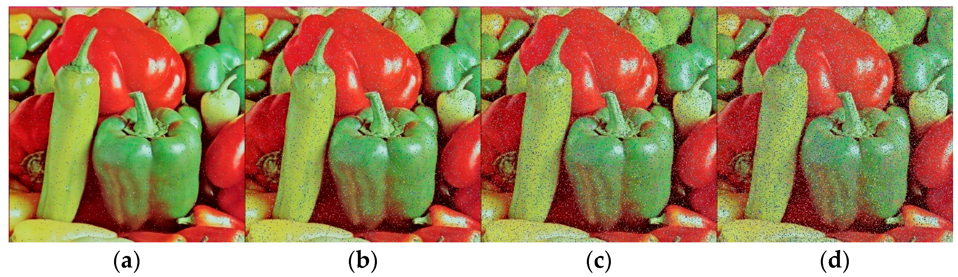
Figure 33.
Decrypted image under different levels of noise attack. (a) Noise density of 0.01. (b) Noise density of 0.05. (c) Noise density of 0.1. (d) Noise density of 0.15.
Figure 33.
Decrypted image under different levels of noise attack. (a) Noise density of 0.01. (b) Noise density of 0.05. (c) Noise density of 0.1. (d) Noise density of 0.15.
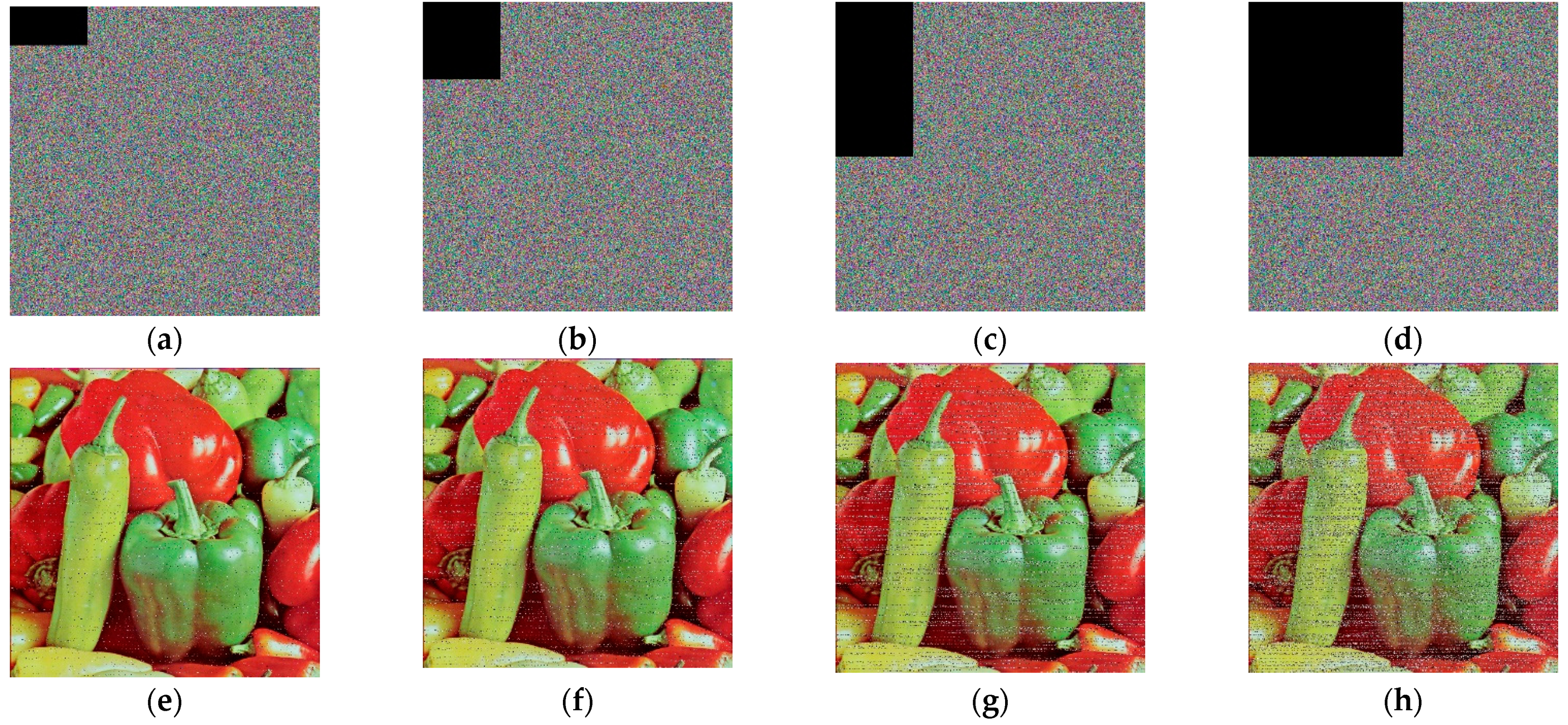
Figure 34.
Anti-occlusion attack detection for Pepper image. (a–d) Various levels of occluded images. (e–h) Decrypted images of (a–d).
Figure 34.
Anti-occlusion attack detection for Pepper image. (a–d) Various levels of occluded images. (e–h) Decrypted images of (a–d).
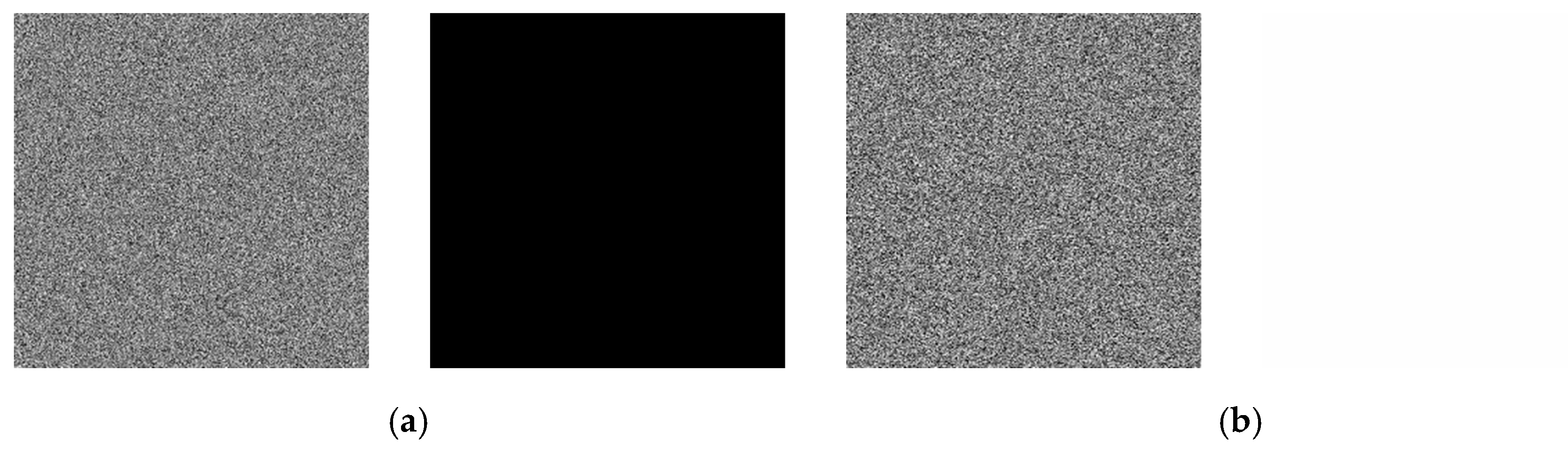
Figure 35.
Chosen-plaintext attack test results. (a) Encryption and decryption of all-black image. (b) Encryption and decryption image of all-white image.
Figure 35.
Chosen-plaintext attack test results. (a) Encryption and decryption of all-black image. (b) Encryption and decryption image of all-white image.
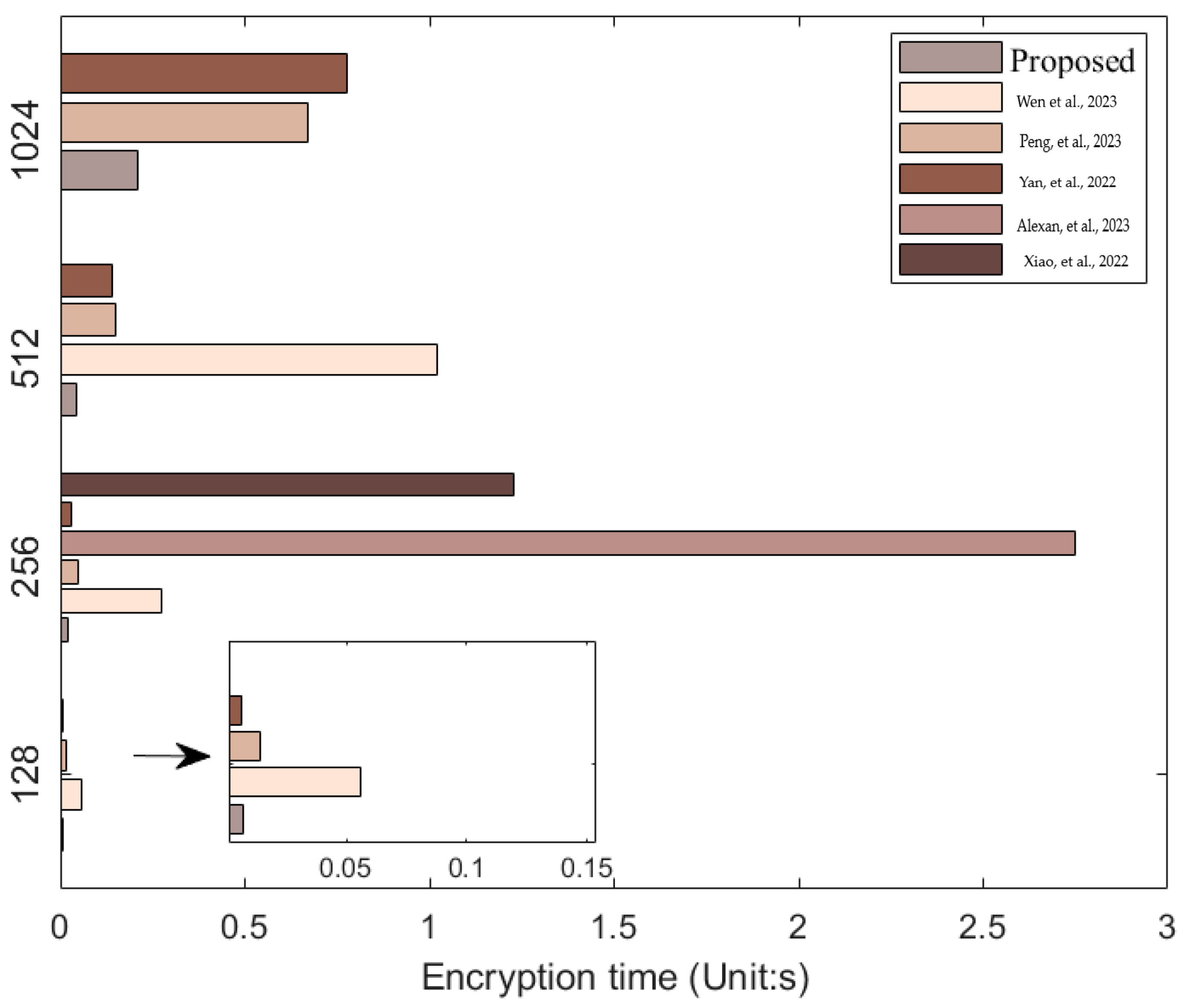
Figure 36.
Comparison of encryption times for different algorithms (Unit: s) [
49,
50,
51,
52,
53].
Figure 36.
Comparison of encryption times for different algorithms (Unit: s) [
49,
50,
51,
52,
53].
Table 1.
NIST test of proposed 3D chaotic system.
Table 1.
NIST test of proposed 3D chaotic system.
| Test | p-Value (X) | p-Value (Y) | p-Value (Z) | State |
|---|
| Frequency | 0.2653 | 0.2460 | 0.9793 | PASS |
| BlockFrequency | 0.7785 | 0.4092 | 0.4190 | PASS |
| CumulativeSums | 0.8331 | 0.9437 | 0.6171 | PASS |
| Runs | 0.1059 | 0.9967 | 0.5615 | PASS |
| LongestRun | 0.0240 | 0.2106 | 0.6260 | PASS |
| NonOverlappingTemplate | 0.9768 | 0.3383 | 0.9537 | PASS |
| Serial | 0.8222 | 0.3072 | 0.1387 | PASS |
| LinearComplexity | 0.9772 | 0.9043 | 0.9307 | PASS |
| RandomExcursions | 0.4870 | 0.6111 | 0.8557 | PASS |
| RandomExcursionsVariant | 0.5523 | 0.7880 | 0.4997 | PASS |
| ApproximateEntropy | 0.0785 | 0.1275 | 0.6155 | PASS |
| Universal | 0.1756 | 0.5527 | 0.6179 | PASS |
| FFT | 1.0000 | 0.4009 | 0.4420 | PASS |
| Rank | 0.2272 | 0.1482 | 0.4449 | PASS |
| OverlappingTemplate | 0.4878 | 0.2704 | 0.5078 | PASS |
Table 2.
Data decomposition rules.
Table 2.
Data decomposition rules.
| Input Data | Output Data |
|---|
| [15-0bit]x | [7-0bit]x | [15-8bit]x |
| [15-0bit]y | [7-0bit]y | [15-8bit]y |
| [15-0bit]z | [7-0bit]z | [15-8bit]z |
Table 3.
Evaluation function decision table.
Table 3.
Evaluation function decision table.
| | E1 | C1 | T1 | S1 |
|---|
| ideal solution | 8 | 0 | 0 | 0 |
| negative ideal solution | 6.5 | 1 | 10 | 1 |
Table 4.
The data of test images.
Table 4.
The data of test images.
| Name of the Image | Image Type | Image Size |
|---|
| Cameraman.bmp | Grayscale image | 256 × 256 |
| Baboon.jpg | Color image | 256 × 256 |
| House.png | Color image | 256 × 256 |
| Airplane.bmp | Color image | 512 × 512 |
| Pepper.tiff | Color image | 512 × 512 |
Table 5.
Different images Test data results.
Table 5.
Different images Test data results.
| Image | Test |
|---|
| R | G | B |
|---|
| Baboon (256 × 256) | 236.8828 | 248.0649 | 255.3281 |
| House (256 × 256) | 260.0078 | 264.8750 | 223.5625 |
| Airplane (512 × 512) | 251.3828 | 241.2832 | 252.7246 |
| Pepper (512 × 512) | 231.4551 | 232.3555 | 248.7051 |
Table 6.
Information entropy of plaintext image and ciphertext image.
Table 6.
Information entropy of plaintext image and ciphertext image.
| Image/Size | RGB Components of the Image | Information Entropy of Plaintext Image | Information Entropy of Ciphertext Image |
|---|
| Cameraman.bmp (256 × 256) | - | 7.0097 | 7.9974 |
| | R | 7.5856 | 7.9974 |
| Baboon.jpg | G | 7.8284 | 7.9973 |
| 256 × 256 | B | 7.3319 | 7.9972 |
| | R | 6.4311 | 7.9974 |
| House.png | G | 6.5389 | 7.9977 |
| 256 × 256 | B | 6.2320 | 7.9977 |
| | R | 6.7178 | 7.9993 |
| Airplane.bmp | G | 6.7990 | 7.9993 |
| 512 × 512 | B | 6.6390 | 7.9994 |
| | R | 7.3319 | 7.9994 |
| Pepper.tiff | G | 7.5254 | 7.9993 |
| 512 × 512 | B | 7.0973 | 7.9994 |
Table 7.
Comparison of information entropy with other algorithms.
Table 7.
Comparison of information entropy with other algorithms.
| | Encryption Algorithm | R | G | B |
|---|
Pepper.png
(512 × 512) | Proposed | 7.9994 | 7.9993 | 7.9994 |
| Ref. [49] | 7.9993 | 7.9993 | 7.9994 |
House.png
(256 × 256) | Proposed | 7.9974 | 7.9977 | 7.9977 |
| Ref. [50] | 7.9970 | 7.9976 | 7.9975 |
Airplane.bmp
(512 × 512) | Proposed | 7.9993 | 7.9993 | 7.9994 |
| Ref. [51] | 7.9993 | 7.9992 | 7.9994 |
Baboon.jpg
(256 × 256) | Proposed | 7.9974 | 7.9973 | 7.9972 |
| Ref. [52] | 7.9965 | 7.9963 | 7.9967 |
Table 8.
Comparison with correlation coefficients of other studies.
Table 8.
Comparison with correlation coefficients of other studies.
| Correlation | This Paper | Ref. [53] | Ref. [49] | Ref. [52] | Ref. [51] | Ref. [50] | Ref. [54] |
|---|
|
Red Channel
| | | | | | | |
|
Horizontal
|
−0.0011
|
0.0030
|
−
0.0050
|
0.00073
|
−0.0049
|
−
0.0013
|
−0.0050
|
|
Vertical
|
−
0.0014
|
−0.0022
|
−
0.0084
|
0.00311
|
−0.0174
|
−
0.0111
|
−0.0025
|
|
Diagonal
|
0.0005
|
0.0006
|
−0.0062
|
−0.00508
|
0.0045
|
0.0046
|
0.0035
|
|
Green Channel
| | | | | | | |
|
Horizontal
|
−0.0016
|
−0.0091
|
0.0163
|
−0.00054
|
0.0011
|
0.0135
|
−0.0096
|
|
Vertical
|
−0.0004
|
−0.0129
|
−0.0101
|
0.00076
|
−0.0156
|
0.0064
|
−0.0032
|
|
Diagonal
|
0.0007
|
0.0043
|
0.0117
|
0.00331
|
−0.0160
|
−0.0241
|
−0.0023
|
|
Blue Channel
| | | | | | | |
|
Horizontal
|
−0.0013
|
−0.0113
|
−0.0162
|
0.00147
|
−0.0045
|
0.0179
|
0.0018
|
|
Vertical
|
−0.0029
|
−0.0038
|
0.0273
|
−0.00147
|
−0.0175
|
0.0131
|
0.0015
|
|
Diagonal
|
−0.0031
|
−0.0164
|
0.0256
|
0.006219
|
0.0018
|
0.0023
|
−0.0042
|
Table 9.
Comparison of NPCR and UAIC results for Lena color image.
Table 9.
Comparison of NPCR and UAIC results for Lena color image.
| Encryption Algorithm | NPCR (%) | UACI (%) |
|---|
| R | G | B | R | G | B |
|---|
| Proposed | 99.6110 | 99.6068 | 99.6030 | 33.4318 | 33.4552 | 33.4678 |
| Ref. [49] | 99.6826 | 99.6170 | 99.5773 | 33.5152 | 33.5370 | 33.3782 |
| Ref. [52] | 99.6245 | 99.6245 | 99.6245 | 33.0704 | 30.7620 | 27.8720 |
| Ref. [51] | 99.6257 | 99.6145 | 99.6257 | 33.4892 | 33.4798 | 33.4916 |
| Ref. [50] | 99.6429 | 99.6628 | 99.6261 | 33.4440 | 33.4876 | 33.4167 |
| Ref. [54] | 99.6116 | 99.6052 | 99.6070 | 33.4382 | 33.4862 | 33.4426 |
Table 10.
Calculation of PSNR and SSIM of images after adding different levels of noise.
Table 10.
Calculation of PSNR and SSIM of images after adding different levels of noise.
| Noise Intensity | PSNR | SSIM |
|---|
| 0.01 | 25.4208 | 0.9454 |
| 0.05 | 19.1361 | 0.7984 |
| 0.1 | 16.3294 | 0.6637 |
| 0.15 | 14.7205 | 0.5627 |
Table 11.
Calculation of PSNR and SSIM for images with different levels of Occlusion.
Table 11.
Calculation of PSNR and SSIM for images with different levels of Occlusion.
| Occluded Degree | PSNR | SSIM |
|---|
| 1/32 | 23.1124 | 0.9169 |
| 1/16 | 20.1185 | 0.8483 |
| 1/8 | 17.1374 | 0.7400 |
| 1/4 | 14.0933 | 0.5578 |
Table 12.
Information entropy and correlation coefficients for test images.
Table 12.
Information entropy and correlation coefficients for test images.
| | | Information Entropy | Correlation |
|---|
| | Horizontal | Vertical | Diagonal |
|---|
| All-black encrypted image | 283.5584 | 7.9993 | −0.0049 | −0.0051 | −0.0033 |
| All- white encrypted image | 237.5155 | 7.9991 | −0.0049 | −0.0051 | −0.0033 |
Table 13.
Different-size color image encryption time tests (Unit: s).
Table 13.
Different-size color image encryption time tests (Unit: s).
| Image Types | 256 × 256 | 512 × 512 | 768 × 768 | 1024 × 1024 |
|---|
| Grayscale image | 0.007677 | 0.017778 | 0.038957 | 0.076597 |
| Color image | 0.022775 | 0.046174 | 0.109098 | 0.210875 |
Table 14.
Comparison of encryption times for different algorithms (Unit: s).
Table 14.
Comparison of encryption times for different algorithms (Unit: s).
| Encryption Algorithm | 128 × 128 × 3 | 256 × 256 × 3 | 512 × 512 × 3 | 1024 × 1024 × 3 |
|---|
| Proposed | 0.006990 | 0.020775 | 0.044174 | 0.208875 |
| Ref. [53] | 0.05621 | 0.27413 | 1.01921 | - |
| Ref. [49] | 0.014233 | 0.048602 | 0.151934 | 0.671352 |
| Ref. [52] | - | 2.750966 | - | - |
| Ref. [51] | 0.006679 | 0.03156 | 0.142001 | 0.775764 |
| Ref. [50] | - | 1.2271 | - | - |


