
Attack–Defense Game Model with Multi-Type Attackers Considering Information Dilemma

Abstract
:1. Introduction
2. Related Work
3. Link Hiding Rule and Information Dilemma
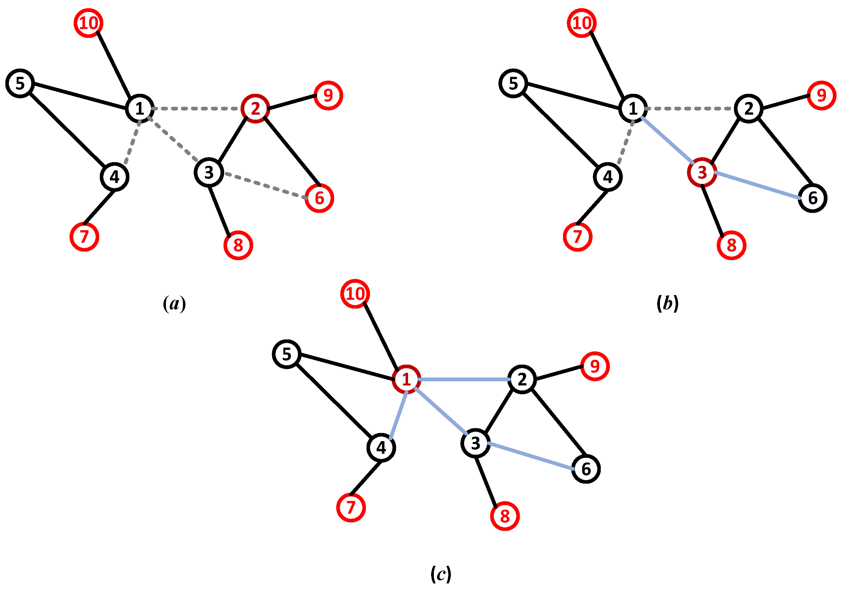
3.1. Link Hiding Rule
3.2. Information Dilemma
4. The Attack–Defense Game Model with Multi-Type Attackers under Information Dilemma
4.1. Cost Model
4.2. Strategy Set
- (1)
- High-degree attack or defense strategy. A high-degree attack strategy damages nodes with a high degree. The high-degree defense strategy defends nodes with a high degree.
- (2)
- Low-degree attack or defense strategy. The low-degree attack strategy is aimed at nodes with a low degree. Because the resources consumed are relatively low compared with high-degree nodes, the low-degree attack at the same cost can destroy more low-degree nodes. The low-degree defense strategy defends nodes with a low degree.
4.3. Payoff Function
5. Solution Method
6. Experiments
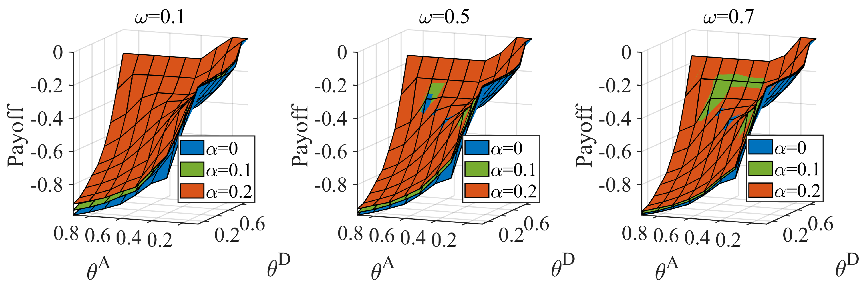
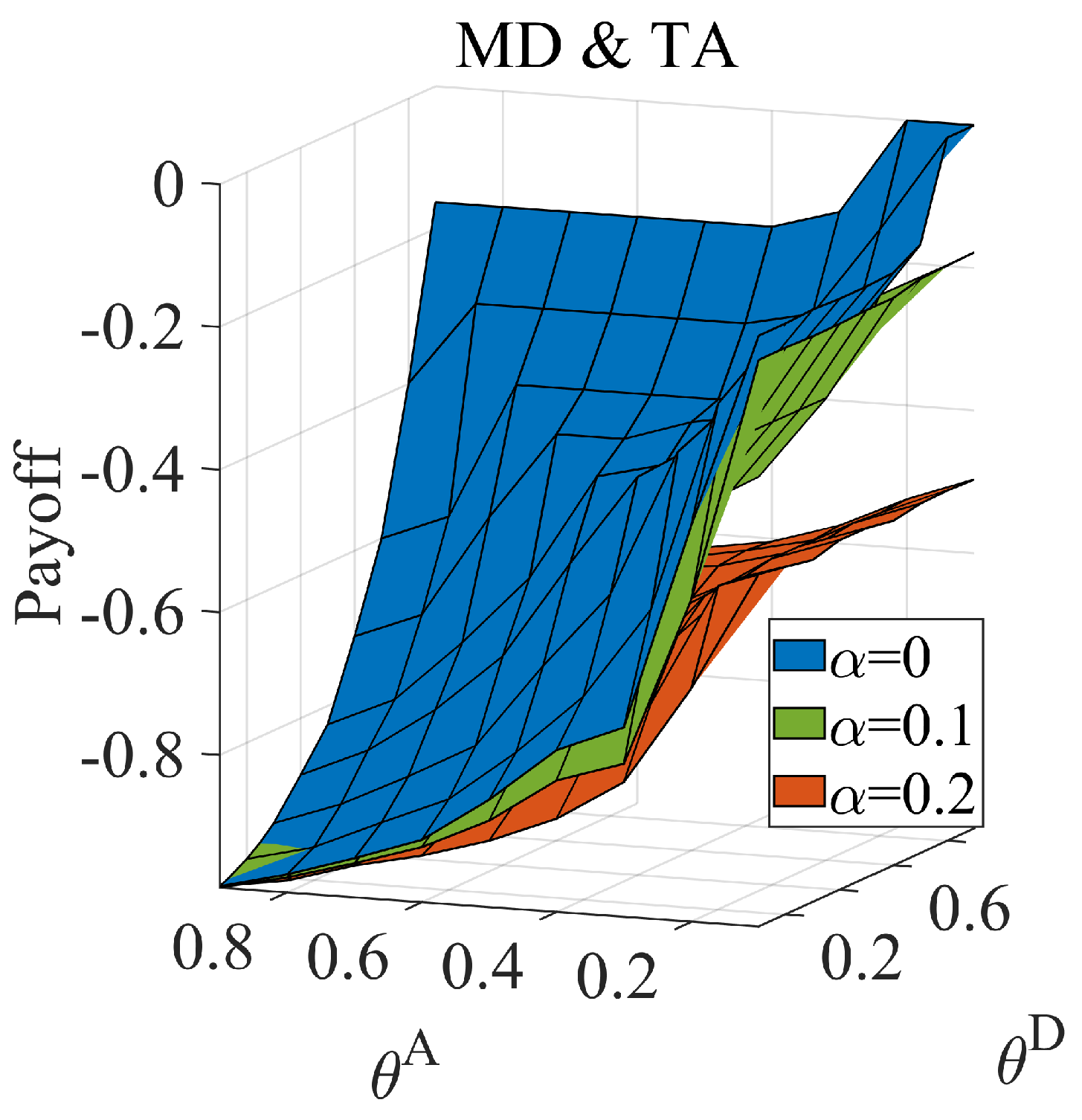
6.1. Benefits of the Link Hiding for the Defender
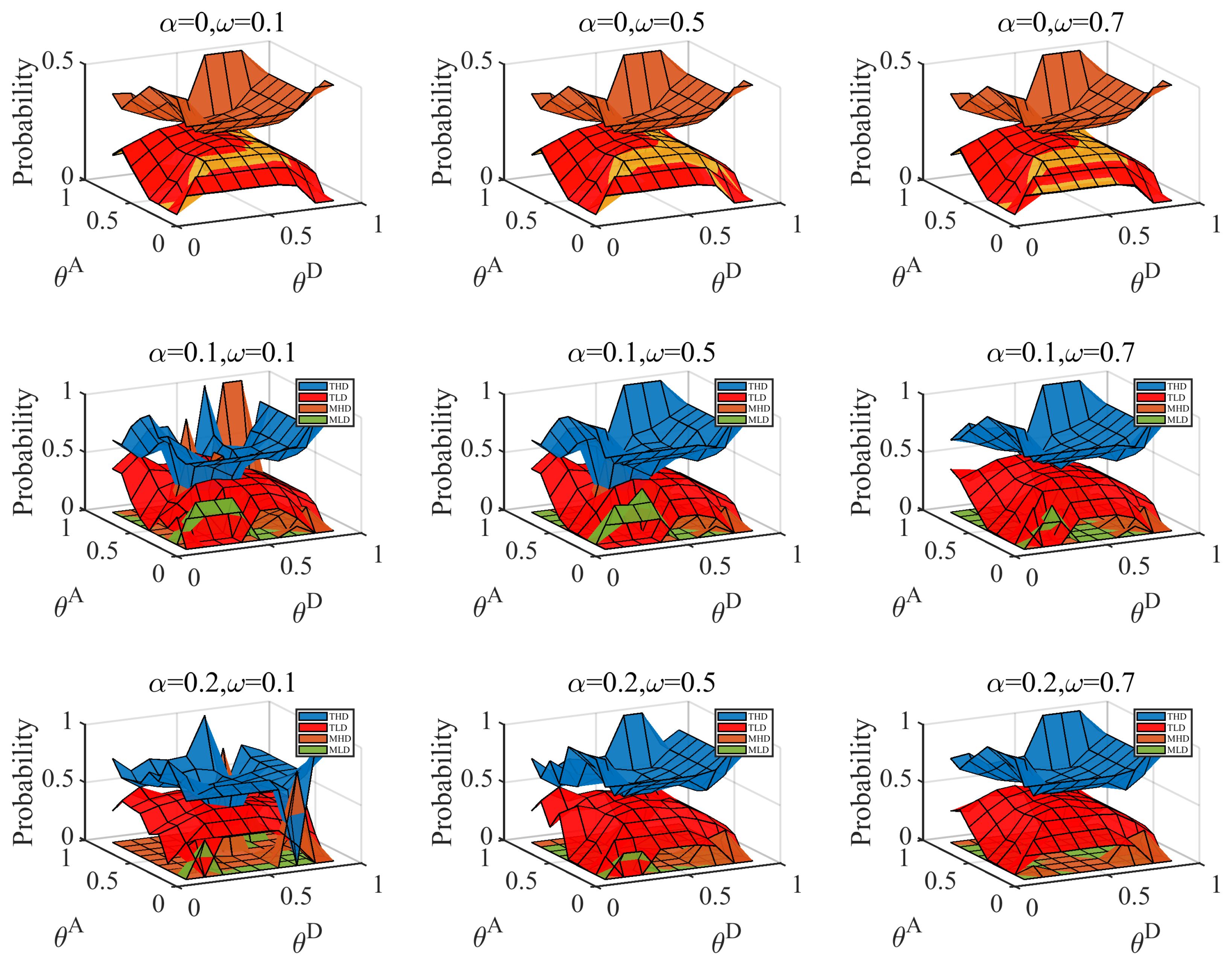
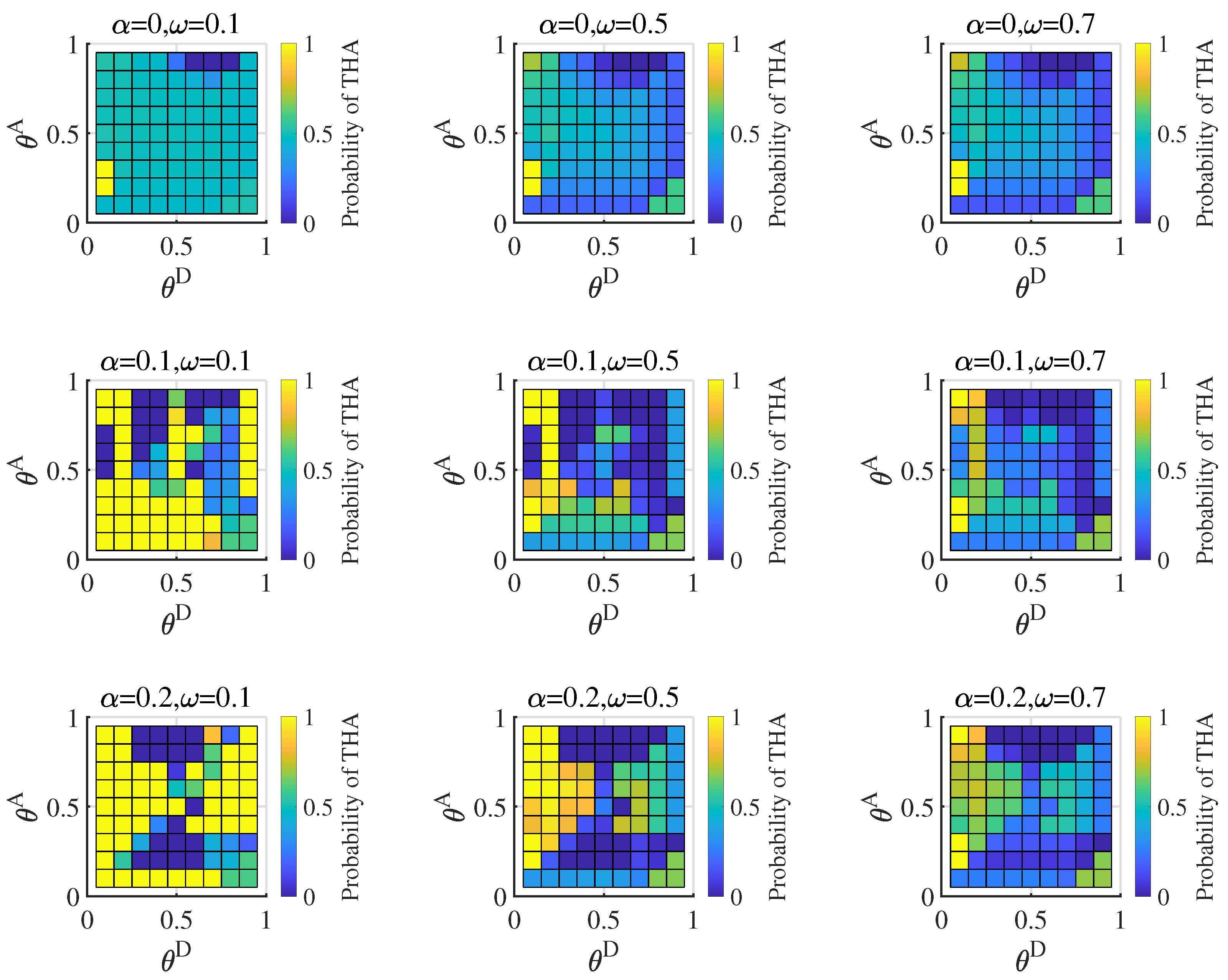
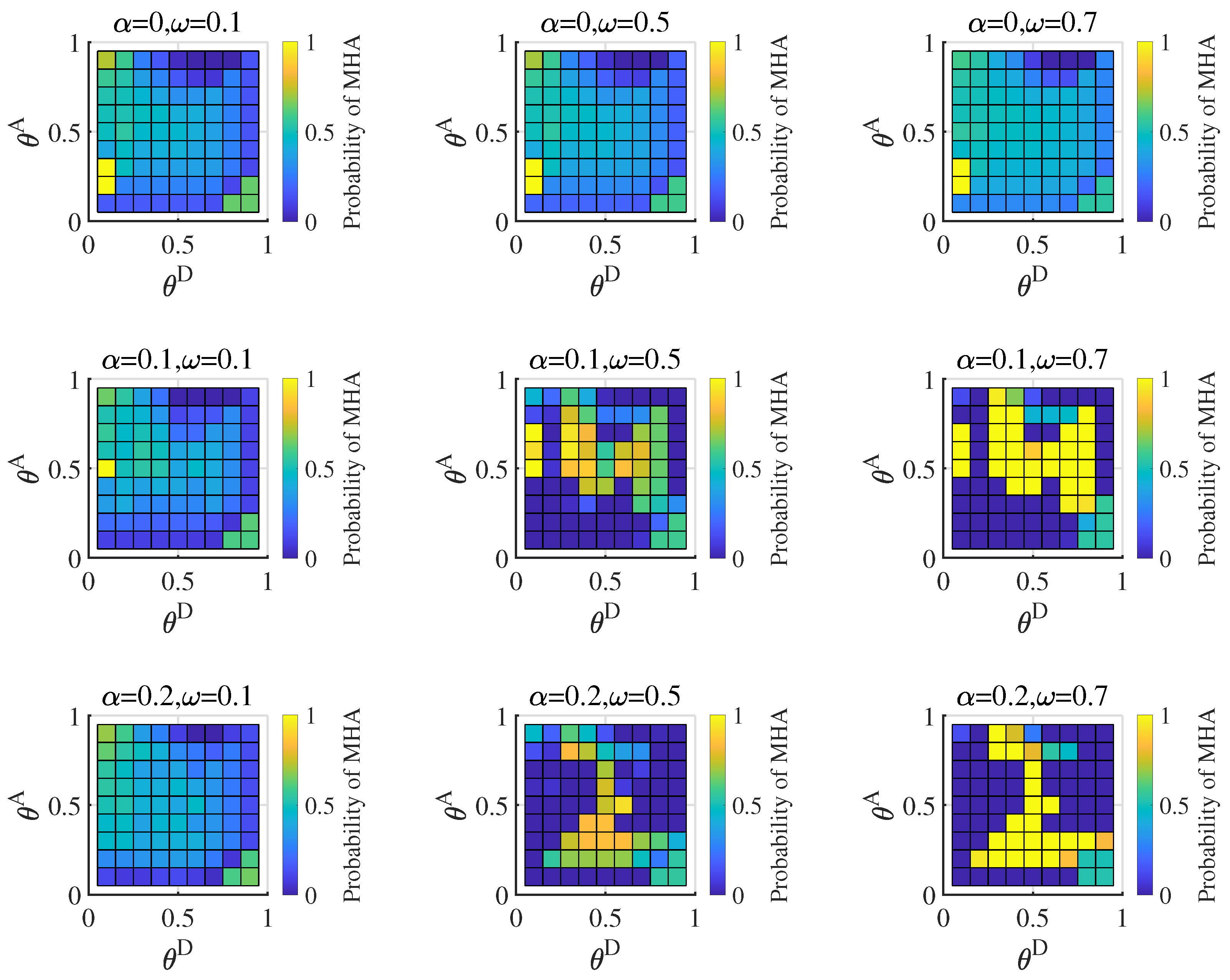
6.2. Equilibrium with Different Distributions of the Attacker’s Type
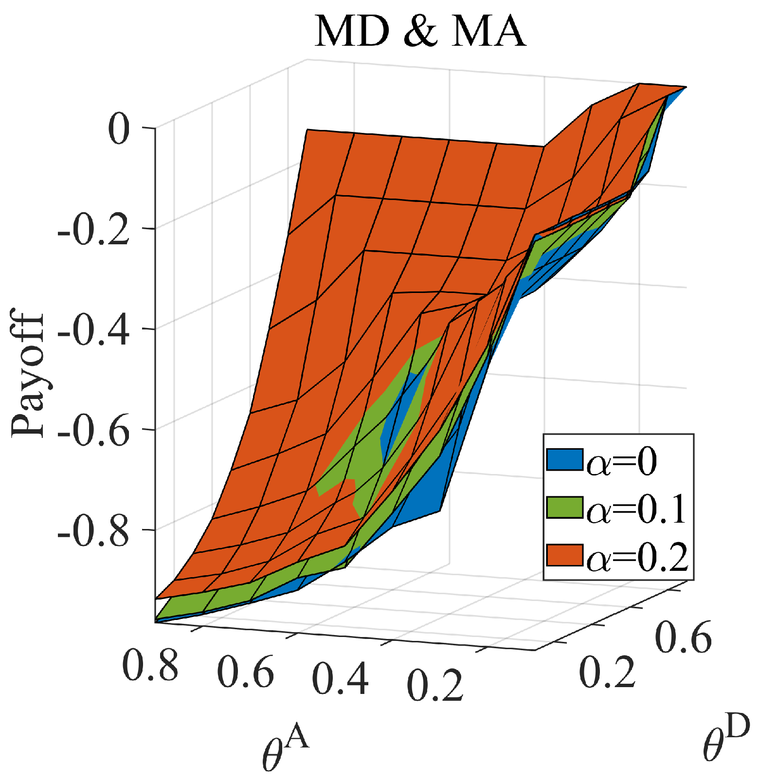
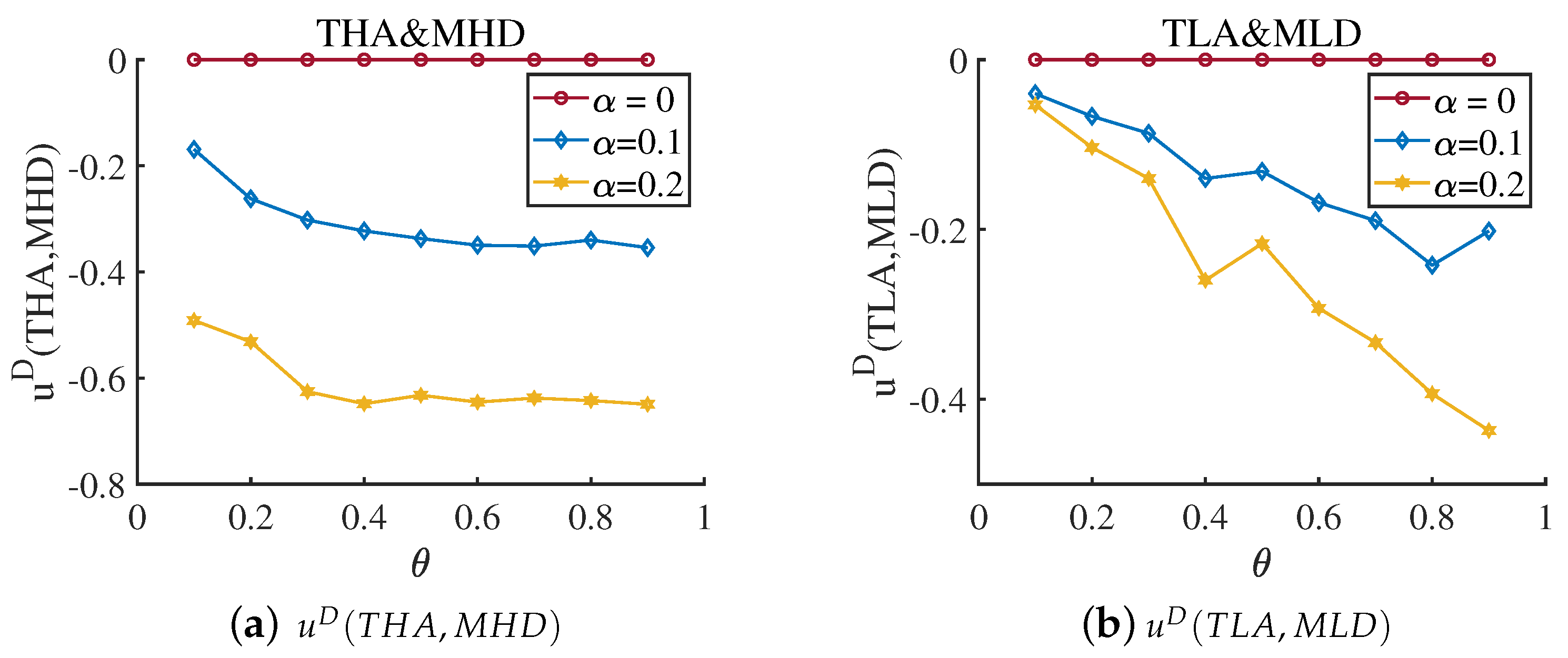
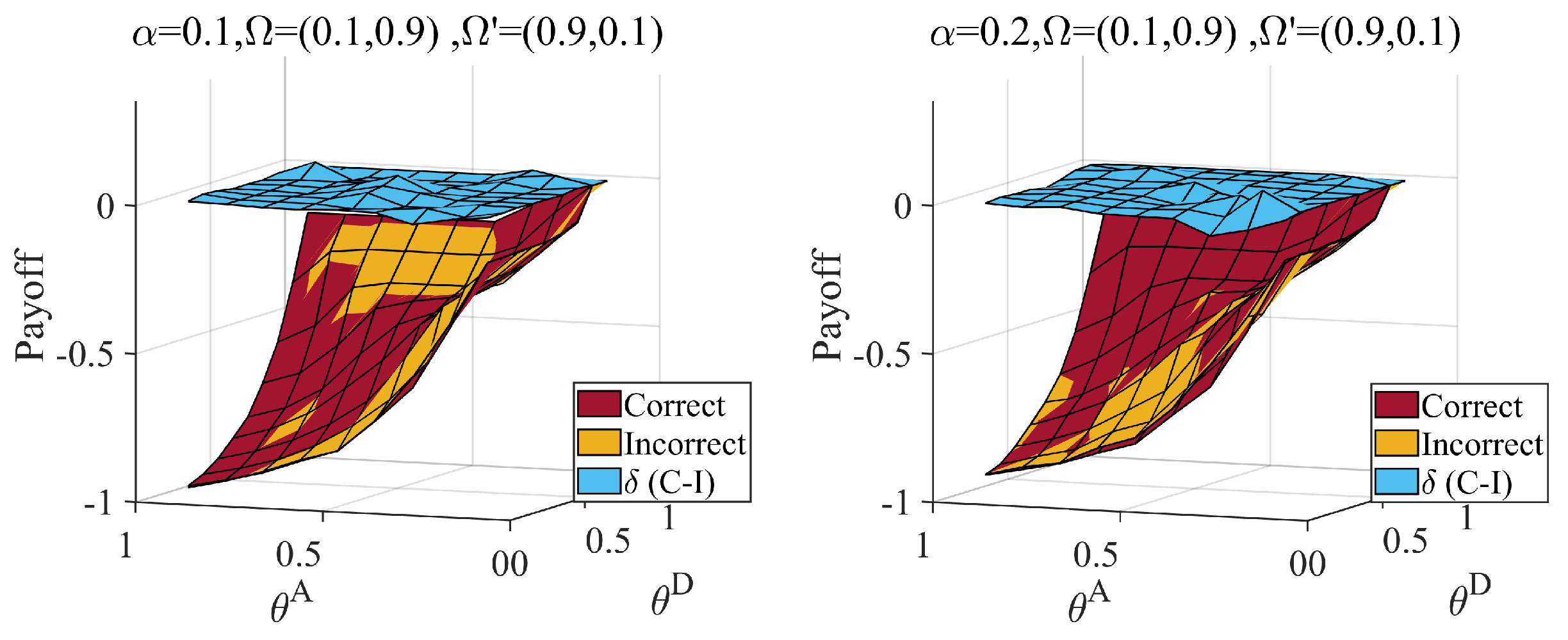
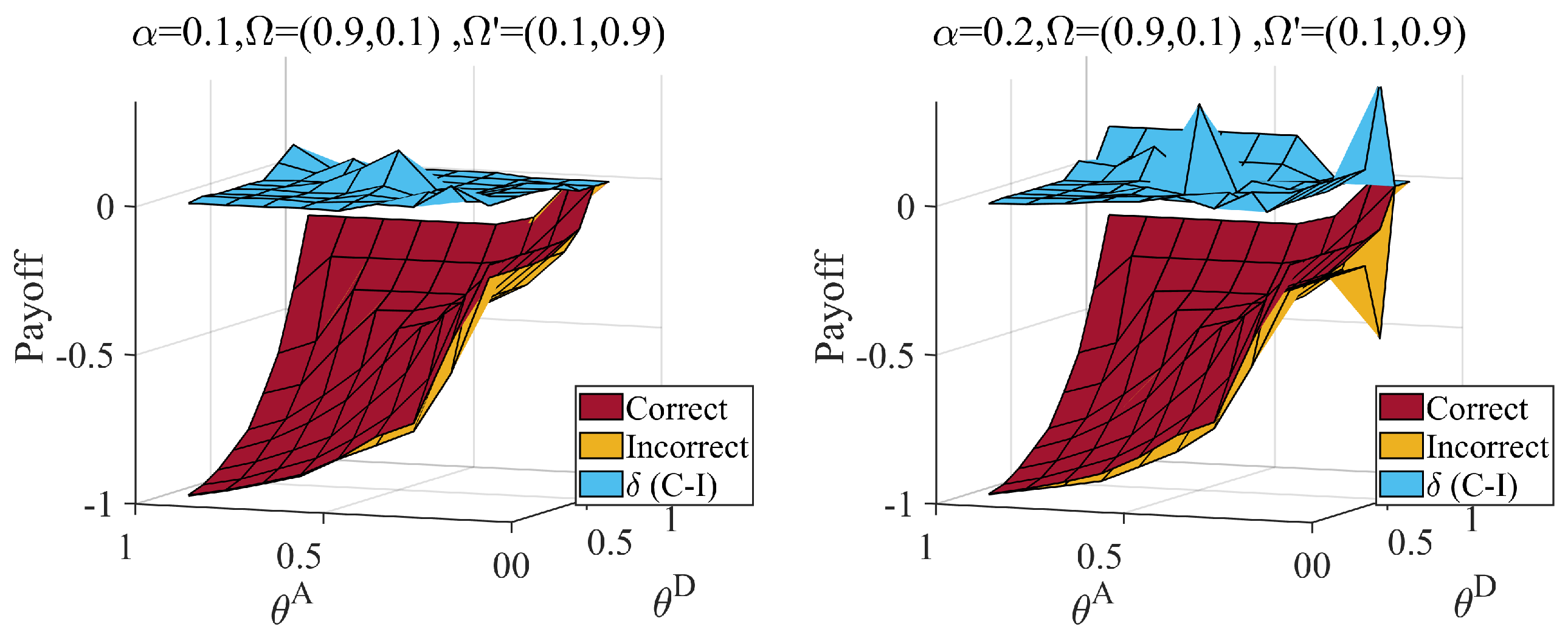
6.3. Influence of the Misjudgment on the Defender
7. Conclusions
Supplementary Materials
Author Contributions
Funding
Institutional Review Board Statement
Informed Consent Statement
Data Availability Statement
Conflicts of Interest
References
- Feng, Q.; Cai, H.; Chen, Z.; Zhao, X.; Chen, Y. Using game theory to optimize allocation of defensive resources to protect multiple chemical facilities in a city against terrorist attacks. J. Loss Prev. Process. Ind. 2016, 43, 614–628. [Google Scholar] [CrossRef]
- Tas, S.; Bier, V.M. Addressing vulnerability to cascading failure against intelligent adversaries in power networks. Energy Syst. 2016, 7, 193–213. [Google Scholar] [CrossRef]
- Talarico, L.; Reniers, G.; Sörensen, K.; Springael, J. MISTRAL: A game-theoretical model to allocate security measures in a multi-modal chemical transportation network with adaptive adversaries. Reliab. Eng. Syst. Saf. 2015, 138, 105–114. [Google Scholar] [CrossRef]
- Li, Y.; Tan, S.; Deng, Y.; Wu, J. Attacker-defender game from a network science perspective. Chaos Interdiscip. J. Nonlinear Sci. 2018, 28, 051102. [Google Scholar] [CrossRef]
- Li, Y.; Deng, Y.; Xiao, Y.; Wu, J. Attack and defense strategies in complex networks based on game theory. J. Syst. Sci. Complex. 2019, 32, 1630–1640. [Google Scholar] [CrossRef]
- Li, Y.; Qiao, S.; Deng, Y.; Wu, J. Stackelberg game in critical infrastructures from a network science perspective. Phys. A Stat. Mech. Its Appl. 2019, 521, 705–714. [Google Scholar] [CrossRef]
- Zeng, C.; Ren, B.; Li, M.; Liu, H.; Chen, J. Stackelberg game under asymmetric information in critical infrastructure system: From a complex network perspective. Chaos Interdiscip. J. Nonlinear Sci. 2019, 29, 083129. [Google Scholar] [CrossRef]
- Zeng, C.; Ren, B.; Liu, H.; Chen, J. Applying the bayesian stackelberg active deception game for securing infrastructure networks. Entropy 2019, 21, 909. [Google Scholar] [CrossRef] [Green Version]
- Qi, G.; Li, J.; Xu, X.; Chen, G.; Yang, K. An attack–defense game model in infrastructure networks under link hiding. Chaos Interdiscip. J. Nonlinear Sci. 2022, 32, 113109. [Google Scholar] [CrossRef]
- Bier, V.; Oliveros, S.; Samuelson, L. Choosing what to protect: Strategic defensive allocation against an unknown attacker. J. Public Econ. Theory 2007, 9, 563–587. [Google Scholar] [CrossRef]
- Baykal-Guersoy, M.; Duan, Z.; Poor, H.V.; Garnaev, A. Infrastructure security games. Eur. J. Oper. Res. 2014, 239, 469–478. [Google Scholar] [CrossRef]
- Chen, P.; Cheng, S.; Chen, K. Smart attacks in smart grid communication networks. IEEE Commun. Mag. 2012, 50, 24–29. [Google Scholar] [CrossRef]
- Fu, C.; Gao, Y.; Zhong, J.; Sun, Y.; Pengtao, Z.; Wu, T. Attack-defense game for critical infrastructure considering the cascade effect. Reliab. Eng. Syst. Saf. 2021, 216, 107958. [Google Scholar]
- Brown, G.; Carlyle, M.; Salmerón, J.; Wood, K. Defending critical infrastructure. Interfaces 2006, 36, 530–544. [Google Scholar] [CrossRef] [Green Version]
- Fu, C.; Zhang, P.; Zhou, L.; Gao, Y.; Du, N. Camouflage strategy of a Stackelberg game based on evolution rules. Chaos Solitons Fractals 2021, 153, 111603. [Google Scholar]
- Zhang, H.; Dingkun, Y.U.; Wang, J.; Han, J.; Wang, N. Security Defence Policy Selection Method Using the Incomplete Information Game Model. China Commun. 2015, 9, 2. [Google Scholar]
- Feng, Q.; Cai, H.; Chen, Z. Using game theory to optimize the allocation of defensive resources on a city scale to protect chemical facilities against multiple types of attackers. Reliab. Eng. Syst. Saf. 2019, 191, 105900. [Google Scholar] [CrossRef]
- Jiang, J.; Liu, X. Bayesian Stackelberg game model for water supply networks against interdictions with mixed strategies. Int. J. Prod. Res. 2021, 59, 2537–2557. [Google Scholar] [CrossRef]
- Gu, X.; Zeng, C.; Xiang, F. Applying a Bayesian Stackelberg game to secure infrastructure system: From a complex network perspective. In Proceedings of the 2019 4th International Conference on Automation, Control and Robotics Engineering, Shenzhen, China, 19–21 July 2019; pp. 1–6. [Google Scholar]
- Li, Y.; Wu, J.; Zou, A. Effect of eliminating edges on robustness of scale-free networks under intentional attack. Chin. Phys. Lett. 2010, 27, 068901. [Google Scholar]
- Hayashi, Y.; Matsukubo, J. Improvement of the robustness on geographical networks by adding shortcuts. Phys. A Stat. Mech. Its Appl. 2007, 380, 552–562. [Google Scholar] [CrossRef] [Green Version]
- Zhou, X.; Chen, Q.; Lyu, S.; Chen, H. Mapping the Buried Cable by Ground Penetrating Radar and Gaussian-Process Regression. IEEE Trans. Geosci. Remote. Sens. 2022, 60, 1–12. [Google Scholar] [CrossRef]
- Harsanyi, J.C.; Selten, R. A generalized Nash solution for two-person bargaining games with incomplete information. Manag. Sci. 1972, 18, 80–106. [Google Scholar] [CrossRef]
- Harsanyi, J.C. Games with incomplete information played by “Bayesian” players, I–III Part I. The basic model. Manag. Sci. 1967, 14, 159–182. [Google Scholar] [CrossRef]
- Harsanyi, J.C. Games with incomplete information played by “Bayesian” players part II. Bayesian equilibrium points. Manag. Sci. 1968, 14, 320–334. [Google Scholar] [CrossRef]
- Bilò, V.; Fanelli, A. Computing exact and approximate Nash equilibria in 2-player games. In Proceedings of the International Conference on Algorithmic Applications in Management; Springer: Berlin/Heidelberg, Germany, 2010; pp. 58–69. [Google Scholar]
- De Masi, G.; Iori, G.; Caldarelli, G. Fitness model for the Italian interbank money market. Phys. Rev. E 2006, 74, 066112. [Google Scholar] [CrossRef] [PubMed] [Green Version]
- Guimera, R.; Mossa, S.; Turtschi, A.; Amaral, L.N. The worldwide air transportation network: Anomalous centrality, community structure, and cities’ global roles. Proc. Natl. Acad. Sci. USA 2005, 102, 7794–7799. [Google Scholar] [CrossRef] [PubMed] [Green Version]
- Zhang, J.; Wang, Y.; Zhuang, J. Modeling multi-target defender-attacker games with quantal response attack strategies. Reliab. Eng. Syst. Saf. 2021, 205, 107165. [Google Scholar] [CrossRef]


| Type | Proficient Attacker | |
|---|---|---|
| Strategy | THA | TLA |
| Type | Normal Attacker | |
|---|---|---|
| Strategy | MHA | MLA |
| Strategy | , | , | , | , |
|---|---|---|---|---|
| Abbreviations | Definitions |
|---|---|
| BNE | Bayesian Nash equilibrium |
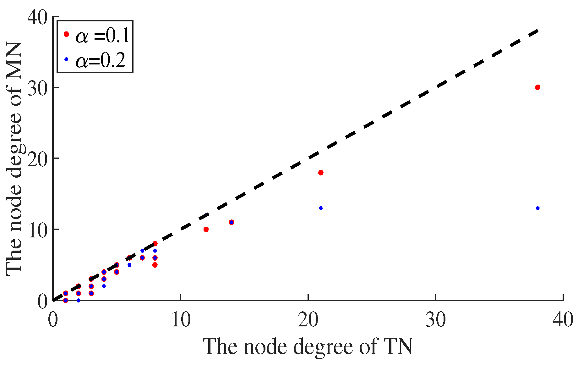
| TN | True network |
| MN | Misleading network |
| High-degree attack strategy based on true networks | |
| Low-degree attack strategy based on true networks | |
| High-degree attack strategy based on misleading networks | |
| Low-degree attack strategy based on misleading networks | |
| High-degree defense strategy based on true networks | |
| Low-degree defense strategy based on true networks | |
| High-degree defense strategy based on misleading networks | |
| Low-degree defense strategy based on misleading networks | |
| Strategy set contains and | |
| Strategy set contains and |
Disclaimer/Publisher’s Note: The statements, opinions and data contained in all publications are solely those of the individual author(s) and contributor(s) and not of MDPI and/or the editor(s). MDPI and/or the editor(s) disclaim responsibility for any injury to people or property resulting from any ideas, methods, instructions or products referred to in the content. |
© 2022 by the authors. Licensee MDPI, Basel, Switzerland. This article is an open access article distributed under the terms and conditions of the Creative Commons Attribution (CC BY) license (https://creativecommons.org/licenses/by/4.0/).
Share and Cite
Qi, G.; Li, J.; Xu, C.; Chen, G.; Yang, K. Attack–Defense Game Model with Multi-Type Attackers Considering Information Dilemma. Entropy 2023, 25, 57. https://doi.org/10.3390/e25010057
Qi G, Li J, Xu C, Chen G, Yang K. Attack–Defense Game Model with Multi-Type Attackers Considering Information Dilemma. Entropy. 2023; 25(1):57. https://doi.org/10.3390/e25010057
Chicago/Turabian StyleQi, Gaoxin, Jichao Li, Chi Xu, Gang Chen, and Kewei Yang. 2023. "Attack–Defense Game Model with Multi-Type Attackers Considering Information Dilemma" Entropy 25, no. 1: 57. https://doi.org/10.3390/e25010057