

Unsupervised Anomaly Detection for Intermittent Sequences Based on Multi-Granularity Abnormal Pattern Mining

Abstract
:1. Introduction
- (1)
- An abnormal volatility metric for intermittent time series is proposed. The index not only considers the difference in volatility patterns between series but also the correlation between series, so as to achieve an the accurate quantification of abnormal volatility of intermittent time series.
- (2)
- An unsupervised anomaly detection method for intermittent sequences based on multi-granularity anomaly pattern mining is constructed. Compared with the traditional anomaly detection methods, the method can identify anomalous sequences by mining the sequence anomaly fluctuation patterns from macroscopic and macroscopic perspectives, and effectively use the information of demand point value change in the sequence to locate the anomalous demand in anomalous sequences, which improves the intermittent sequence detection accuracy.
2. Related Theories
2.1. Demand Model Classification
2.2. Hierarchical Clustering
2.3. SVDD
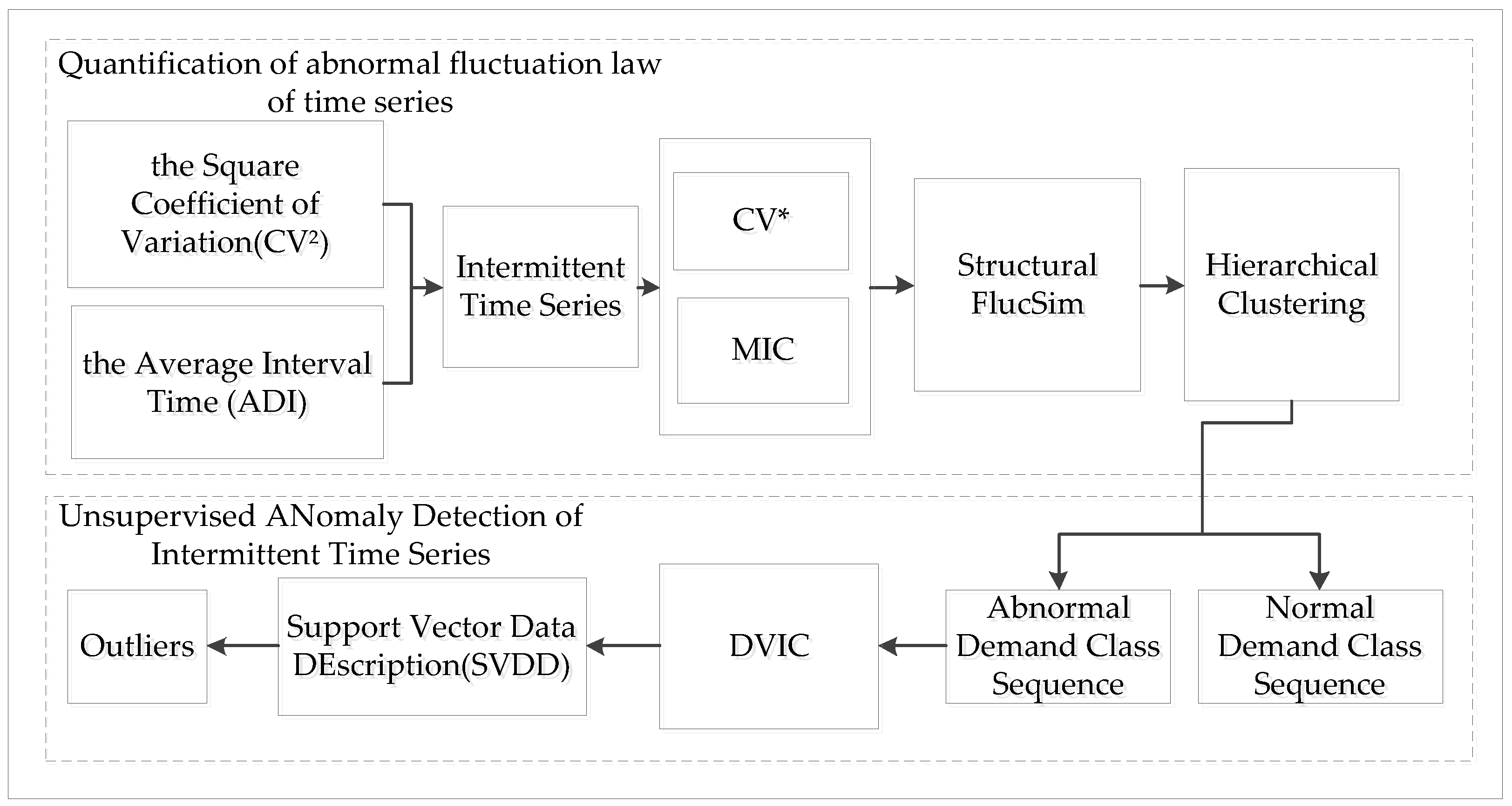
3. Unsupervised Anomaly Detection Method for Intermittent Sequences Based on Multi-Granularity Anomaly Pattern Mining
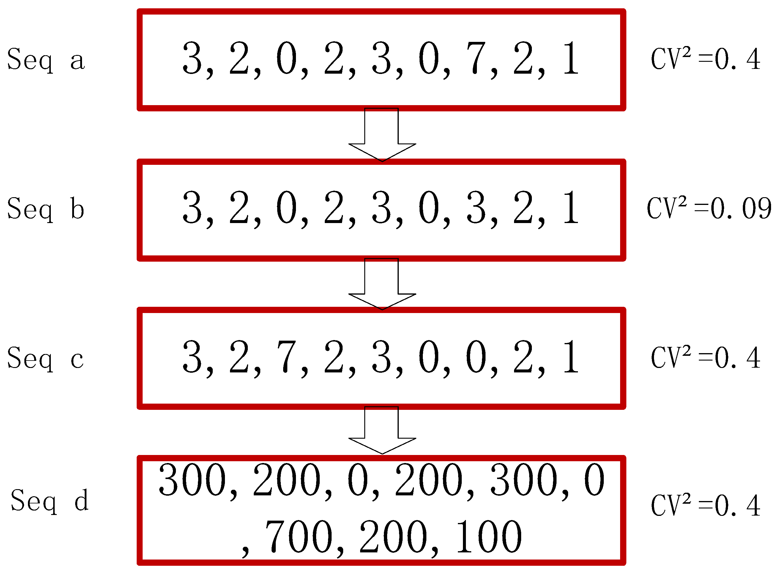
3.1. Construction of Anomalous Fluctuation Similarity Index for Intermittent Series
- (1)
- Partitioning the original dataset based on the and indicators to identify intermittent sequences.
- (2)
- Considering each intermittent sequence as a class cluster.
- (3)
- Calculating the similarity distance between each class cluster using Equation (4).where , and denote the number of sequences contained in the class cluster and the class cluster that participate in the distance calculation, respectively, and denotes the number of sequences.
- (4)
- Merging the two closest class clusters into one class cluster.
- (5)
- Repeating steps (3) (4) until all sample sequences are divided into a set number of classes.
- (6)
- Calculating the of each sequence in the class cluster obtained from step (5), and calculate the average value in each class cluster, with the value exceeding a preset threshold set as an abnormal sequence, and the rest are normal sequences.
3.2. Unsupervised Anomaly Detection Method for Intermittent Sequences Based on Multi-Granularity Anomaly Pattern Mining
- (1)
- Demand change features: the three-dimensional demand change characteristics are obtained by calculating the demand difference between the current time node demand and the previous time node demand , the first two-time node demands and the first three time node demands , which reflect the demand change.
- (2)
- Demand interval features: The length of the demand interval is reflected by calculating the interval between the demand at the non-zero demand time node and the demand at the previous non-zero demand time node , where and represent the length of the sequence . The matrix is shown in Table 1.
- (1)
- Set into a class separately and obtain the class cluster.
- (2)
- Find the two class clusters and with the shortest similarity distance from the class cluster . The formula for calculating the similarity distance is shown below.
- (3)
- Merge the class clusters and into a new class cluster and update the class cluster .
- (4)
- If the class cluster has been divided into class clusters, go to step (5); otherwise loop to step (2).
- (5)
- Calculate the for each sequence in separately and calculate the average for all sequences in each category.
- (6)
- If the average is smaller than the preset threshold, the corresponding class is set to the normal class , and the rest to the abnormal class:
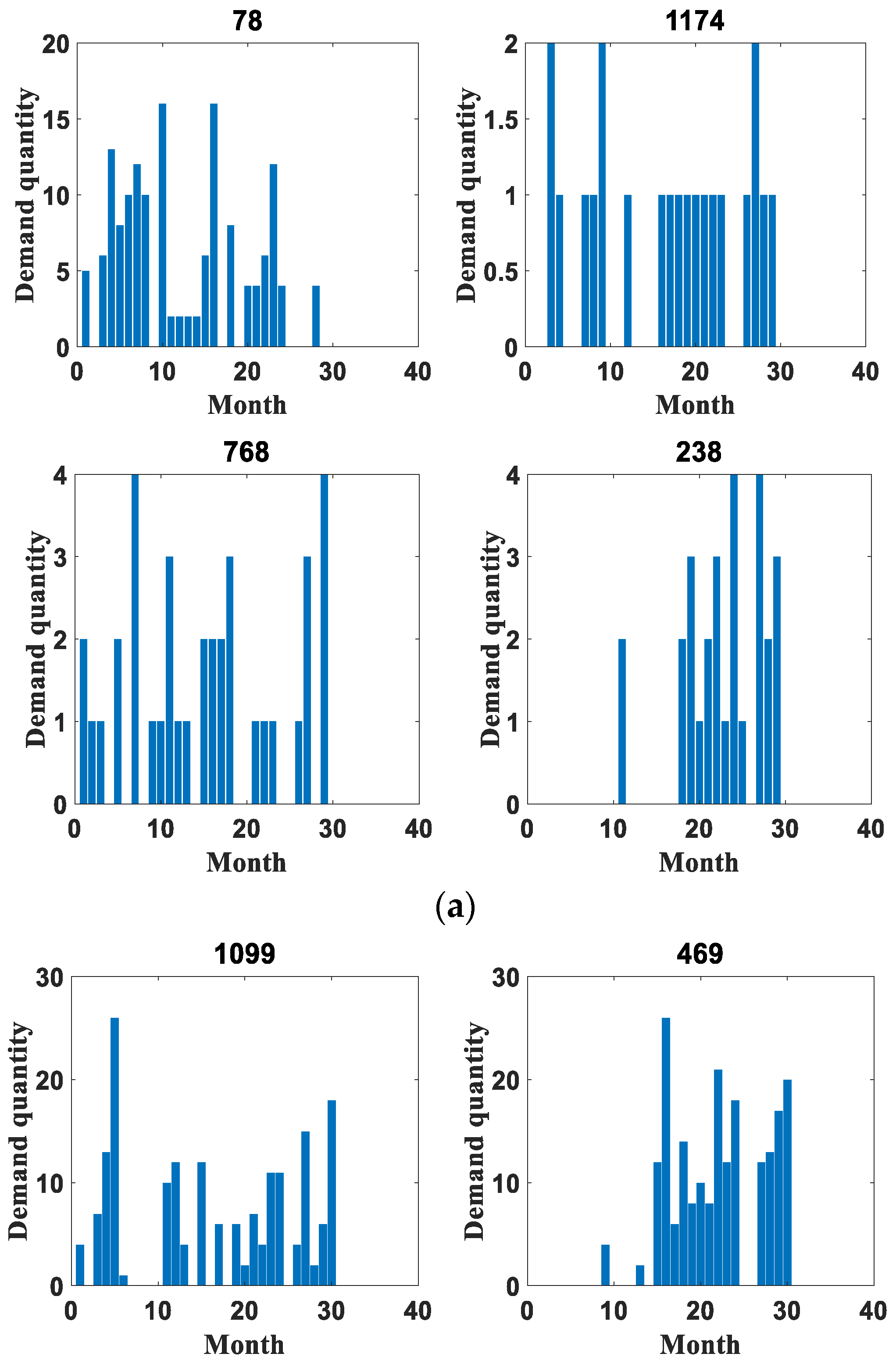
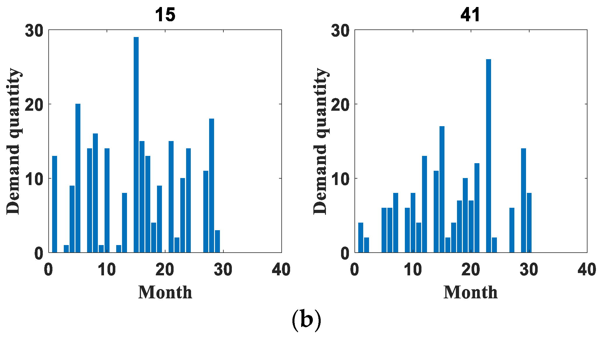
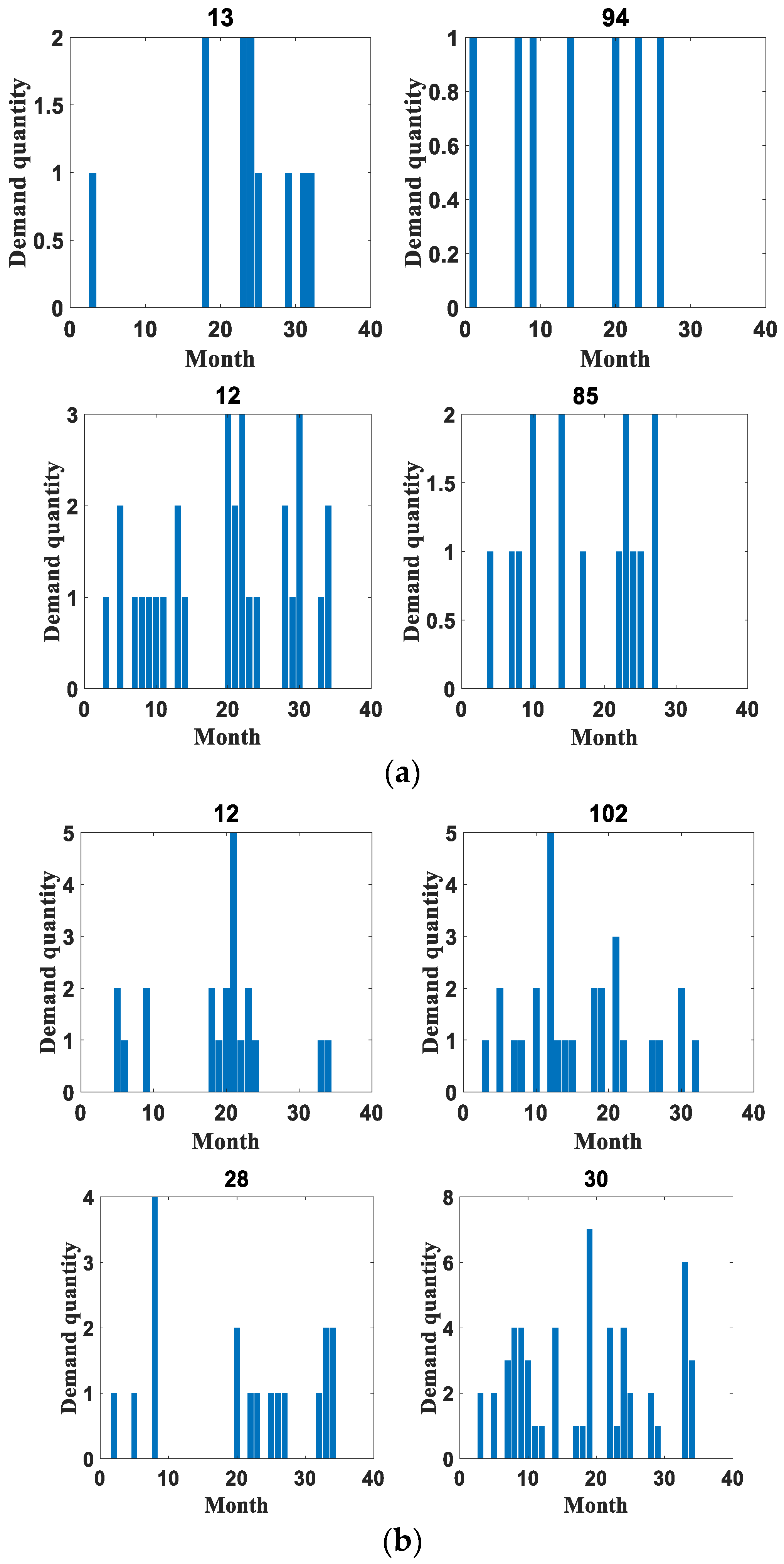
4. Experimental Analysis
4.1. Dataset Introduction

4.2. Evaluation Metrics
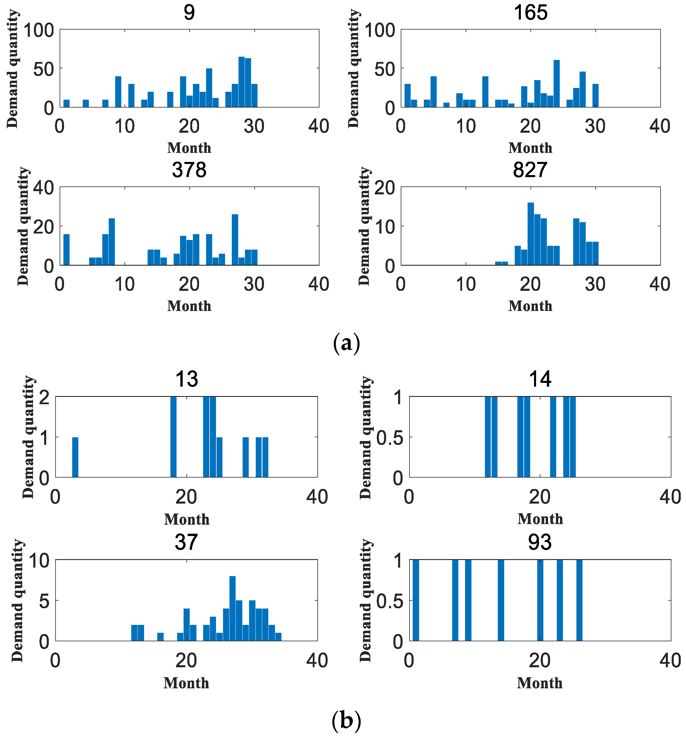
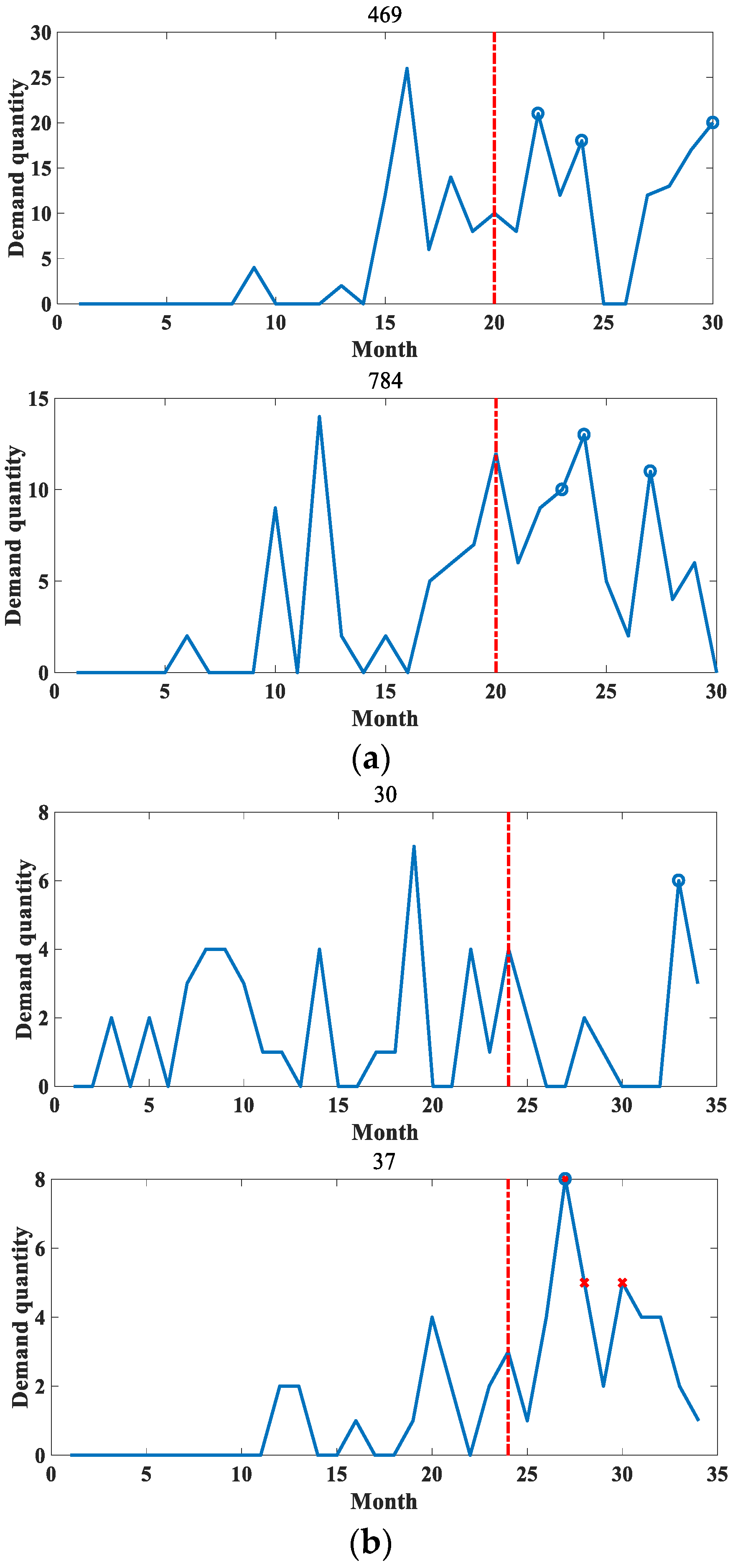
4.3. Experimental Results


4.4. Comparison Method
5. Concluding Remarks
Author Contributions
Funding
Institutional Review Board Statement
Informed Consent Statement
Data Availability Statement
Conflicts of Interest
References
- Ma, M.X.; Mao, W.T.; Fan, L.L.; Lang, Y.P.; Liu, C.H. A Multi-Objective Optimization Model of Safe Inventory for Multi-Level Inventory Collaboration. In Proceedings of the 2020 China Automation Conference (CAC2020), Shanghai, China, 6–8 November 2020; pp. 741–746. [Google Scholar]
- Li, J.; Pedrycz, W.; Jamal, I. Multivariate time series anomaly detection: A framework of Hidden Markov Models. Appl. Soft Comput. 2017, 60, 229–240. [Google Scholar] [CrossRef]
- Lu, W.; Ghorbani, A.A. Network anomaly detection based on wavelet analysis. EURASIP J. Adv. Signal Process. 2008, 2009, 1–16. [Google Scholar] [CrossRef] [Green Version]
- Wang, Z.; Fu, Y.; Song, C.; Zeng, P.; Qiao, L. Power system anomaly detection based on OCSVM optimized by improved particle swarm optimization. IEEE Access 2019, 7, 181580–181588. [Google Scholar] [CrossRef]
- Zhu, J.; Wang, Y.; Zhou, D.; Gao, F. Batch process modeling and monitoring with local outlier factor. IEEE Trans. Control Syst. Technol. 2018, 27, 1552–1565. [Google Scholar] [CrossRef]
- Ramaswamy, S.; Rastogi, R.; Shim, K.; Korea, T. Efficient Algorithms for Mining Outliers from Large Data Sets. In Proceedings of the 2000 ACM SIGMOD International Conference on Management of Data, Dallas, TX, USA, 16–18 May 2000; pp. 427–438. [Google Scholar]
- Liu, F.T.; Ting, K.M.; Zhou, Z.H. Isolation-based anomaly detection. ACM Trans. Knowl. Discov. Data (TKDD) 2012, 6, 1–39. [Google Scholar] [CrossRef]
- Kwon, D.; Kim, H.; Kim, J.; Suh, S.C.; Kim, I.; Kim, K.J. A survey of deep learning-based network anomaly detection. Clust. Comput. 2019, 22, 949–961. [Google Scholar] [CrossRef]
- Niu, Z.; Yu, K.; Wu, X. LSTM-based VAE-GAN for time-series anomaly detection. Sensors 2020, 20, 3738. [Google Scholar] [CrossRef] [PubMed]
- Munir, M.; Siddiqui, S.A.; Dengel, A.; Ahmed, S. DeepAnT: A deep learning approach for unsupervised anomaly detection in time series. IEEE Access 2018, 7, 1991–2005. [Google Scholar] [CrossRef]
- Mor, R.S.; Nagar, J.; Bhardwaj, A. A Comparative Study of Forecasting Methods for Sporadic Demand in An Auto Service Station. Int. J. Bus. Forecast. Mark. Intell. 2019, 5, 56–70. [Google Scholar] [CrossRef]
- Boukhtouta, A.; Jentsch, P. Support Vector Machine for Demand Forecasting of Canadian Armed Forces Spare Parts. In Proceedings of the 2018 IEEE International Symposium on Computational and Business Intelligence (ISCBI); IEEE: Piscataway, NJ, USA, 2018; pp. 59–64. [Google Scholar]
- Reshef, D.N.; Reshef, Y.A.; Finucane, H.K.; Grossman, S.R.; McVean, G.; Turnbaugh, P.J.; Lander, E.S.; Mitzenmacher, M.; Sabeti, P.C. Detecting novel associations in large data sets. Science 2011, 334, 1518–1524. [Google Scholar] [CrossRef]
- Tax, D.M.J.; Duin, R.P.W. Support vector data description. Mach. Learn. 2004, 54, 45–66. [Google Scholar] [CrossRef] [Green Version]
- Syntetos, A.A.; Boylan, J.E. The accuracy of intermittent demand estimates. Int. J. Forecast. 2005, 21, 303–314. [Google Scholar] [CrossRef]
- Lang, Y.; Mao, W.; Luo, T.; Fan, L.; Ren, Y.; Liu, X. Predictability evaluation and joint forecasting method for intermittent time series. J. Comput. Appl. 2022, 42, 2722–2731. [Google Scholar]
- Li, J.; Izakian, H.; Pedrycz, W.; Jamal, I. Clustering-based anomaly detection in multivariate time series data. Appl. Soft Comput. 2021, 100, 106919. [Google Scholar] [CrossRef]
- Wang, P.; Zhang, Z.; Huang, Q.; Wang, N.; Zhang, X.; Lee, W.J. Improved wind farm aggregated modeling method for large-scale power system stability studies. IEEE Trans. Power Syst. 2018, 33, 6332–6342. [Google Scholar] [CrossRef]
- Rakthanmanon, T.; Campana, B.; Mueen, A.; Batista, G.; Westover, B.; Zhu, Q.; Zakaria, J.; Keogh, E. Searching and Mining Trillions of Time Series Subsequences under Dynamic Time Warping. KDD 2012, 2012, 262–270. [Google Scholar] [PubMed] [Green Version]
- Mao, W.; Liu, J.; Chen, J.; Liang, X. An Interpretable Deep Transfer Learning-based Remaining Useful Life Prediction Approach for Bearings with Selective Degradation Knowledge Fusion. IEEE Trans. Instrum. Meas. 2022, 71, 1–16. [Google Scholar] [CrossRef]
- Mao, W.; Ding, L.; Liu, Y.; Afshari, S.S.; Liang, X. A new deep domain adaptation method with joint adversarial training for online detection of bearing early fault. ISA Trans. 2022, 122, 444–458. [Google Scholar] [CrossRef] [PubMed]
- Li, Z.; Zhao, Y.; Botta, N.; Ionescu, C.; Hu, Y.Y. COPOD: Copula-Based Outlier Detection. In Proceedings of the 2020 IEEE International Conference on Data Mining (ICDM), Sorrento, Italy, 17–20 November 2020; pp. 1118–1123. [Google Scholar]


| Original Sequence | Demand Change Characteristics | Demand Interval Characteristics | ||
|---|---|---|---|---|
| Previous Demand Difference | Top Two Demand Differentials | Top Three Demand Differentials | ||
| 0 | 0 | 0 | 0 | 0 |
| 1 | 1 | 0 | 0 | 2 |
| 0 | −1 | 0 | 0 | 0 |
| 1 | 1 | 0 | 1 | 2 |
| 0 | −1 | 0 | −1 | 0 |
| 0 | 0 | −1 | 0 | 0 |
| 0 | 0 | 0 | −1 | 0 |
| 0 | 0 | 0 | 0 | 0 |
| 1 | 1 | 1 | 1 | 5 |
| 0 | −1 | 0 | 0 | 0 |
| 0 | 0 | −1 | 0 | 0 |
| 0 | 0 | 0 | −1 | 0 |
| 0 | 0 | 0 | 0 | 0 |
| 0 | 0 | 0 | 0 | 0 |
| 0 | 0 | 0 | 0 | 0 |
| Dataset | Number of Samples | Number of Features | Properties |
|---|---|---|---|
| Heavy equipment parts requirements dataset | 1200 | 8 | Material number, sales quantity, sales time, number of hosts kept, host type, hours started in the week, number of hosts started in the week, host type |
| A large vehicle manufacturer’s after-sales parts demand dataset | 684 | 4 | Warehouse number, part number, item number, month, monthly demand |
| Dataset | Mean | Standard Deviation | |
|---|---|---|---|
| Heavy equipment parts requirements dataset | Min | 0.4988 | 0.6515 |
| Mode | 1.007 | 1.2143 | |
| Median | 1.669 | 1.7983 | |
| Max | 93.7312 | 132.0505 | |
| A large vehicle manufacturer’s after-sales parts demand dataset | Min | 0.324 | 0.648 |
| Mode | 0.5277 | 1.4133 | |
| Median | 0.4842 | 1.1151 | |
| Max | 1.6129 | 5.595 |
| Algorithm Type | Algorithm Name |
|---|---|
| Linear model | OCSVM [4] |
| Based on density | LOF [5] |
| Based on distance | KNN [6] |
| Based on statistics | COPOD [22] |
| Tree based | IForest [7] |
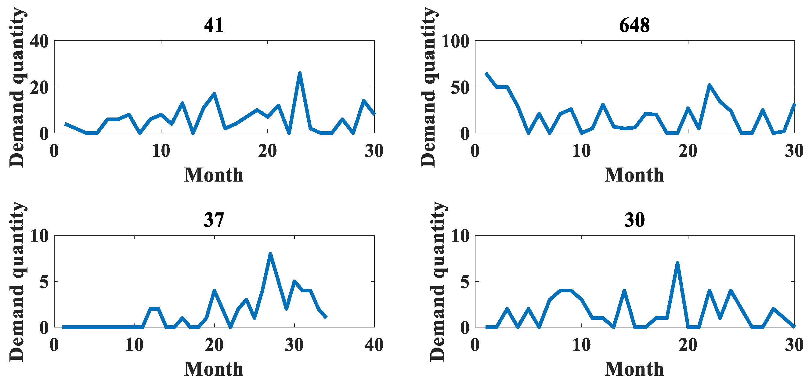
| Accessory Number | Algorithm Name | Time Node Detection Results | Performance Index % | |||||||||||
|---|---|---|---|---|---|---|---|---|---|---|---|---|---|---|
| 21 | 22 | 23 | 24 | 25 | 26 | 27 | 28 | 29 | 30 | Precision | Recall | F1 | ||
| 41 | Real Tags | - | - | o | - | - | - | - | - | o | - | |||
| OCSVM | o | - | o | - | - | - | - | - | o | - | 100.00 | 87.50% | 93.33 | |
| IForest | o | - | o | - | - | - | - | - | o | - | 100.00 | 87.50 | 93.33 | |
| KNN | - | - | o | - | - | - | - | - | o | - | 100.00 | 100.00 | 100.00 | |
| LOF | - | - | o | - | - | - | - | - | - | - | 88.89 | 100.00 | 94.12 | |
| COPOD | - | - | o | - | - | - | - | - | o | - | 100.00 | 100.00 | 100.00 | |
| Methodology of this article | - | - | o | - | - | - | - | - | o | - | 100.00 | 100.00 | 100.00 | |
| 648 | Real Tags | - | o | - | - | - | - | - | - | - | - | |||
| OCSVM | - | o | o | o | - | - | o | - | o | o | 100.00 | 44.44 | 61.54 | |
| IForest | - | o | - | - | - | - | - | - | - | - | 100.00 | 100.00 | 100.00 | |
| KNN | - | - | - | - | - | - | - | - | - | - | 90.00 | 100.00 | 94.74 | |
| LOF | - | - | - | - | - | - | - | - | - | - | 90.00 | 100.00 | 94.74 | |
| COPOD | - | o | - | - | - | - | - | - | - | - | 100.00 | 100.00 | 100.00 | |
| Methodology of this article | - | o | - | - | - | - | - | - | - | - | 100.00 | 100.00 | 100.00 | |
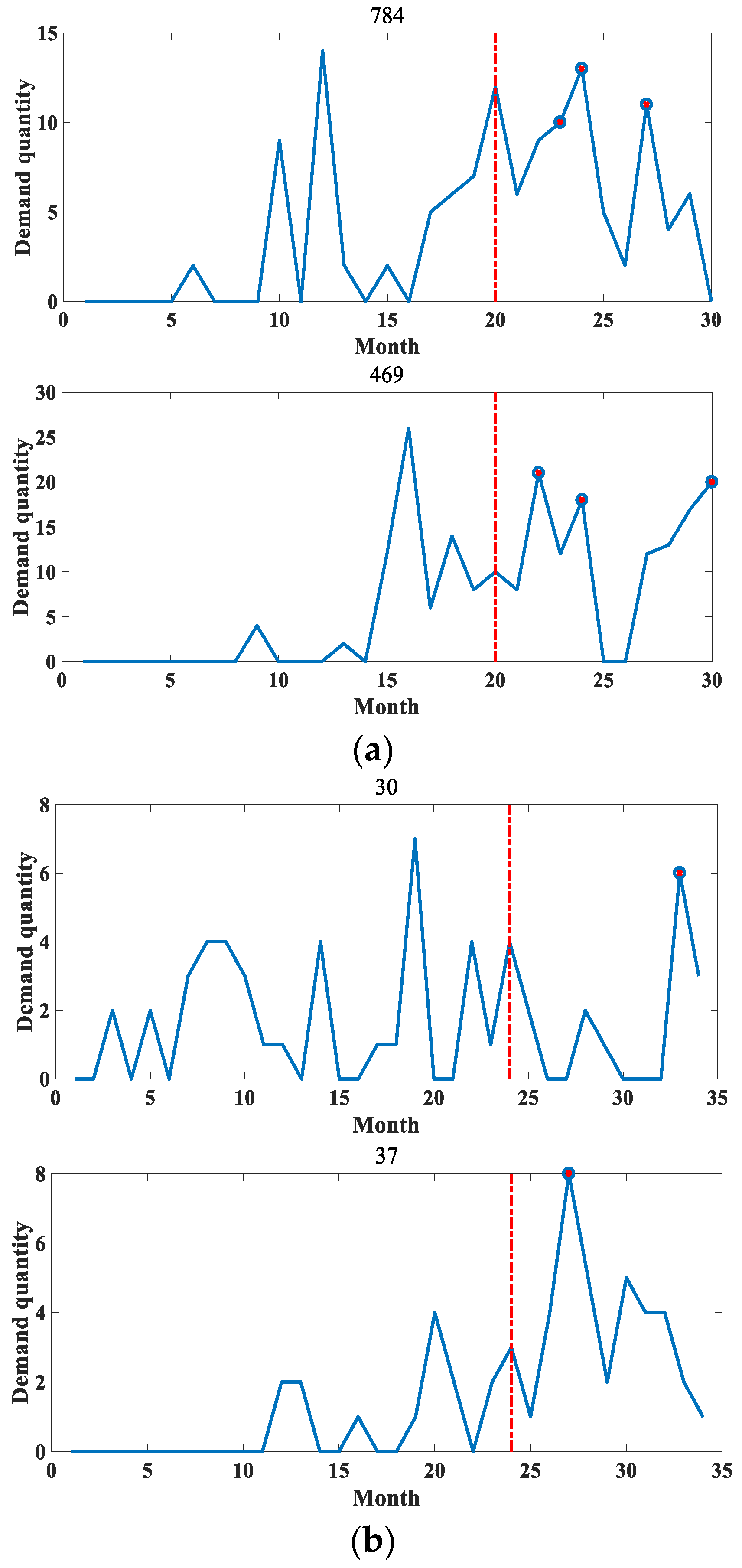
| Accessory Number | Algorithm Name | Time Node Detection Results | Performance Index % | |||||||||||
|---|---|---|---|---|---|---|---|---|---|---|---|---|---|---|
| 25 | 26 | 27 | 28 | 29 | 30 | 31 | 32 | 33 | 34 | Precision | Recall | F1 | ||
| 37 | Real Tags | - | - | o | - | - | - | - | - | - | - | |||
| OCSVM | - | o | o | o | - | o | o | o | - | - | 100.00 | 44.44 | 61.54 | |
| IForest | - | o | o | o | - | o | o | o | - | - | 100.00 | 44.44 | 61.54 | |
| KNN | - | o | o | o | - | o | o | o | - | - | 100.00 | 44.44 | 61.54 | |
| LOF | - | o | o | o | - | o | o | o | - | - | 100.00 | 44.44 | 61.54 | |
| COPOD | - | o | o | o | - | o | o | o | - | - | 100.00 | 44.44 | 61.54 | |
| Methodology of this article | - | - | o | - | - | - | - | - | - | - | 100.00 | 100.00 | 100.00 | |
| 30 | Real Tags | - | - | - | - | - | - | - | - | o | - | |||
| OCSVM | o | - | - | o | - | - | - | - | o | - | 100.00 | 77.78 | 87.50 | |
| IForest | o | - | - | o | - | - | - | - | o | - | 100.00 | 77.78 | 87.50 | |
| KNN | - | - | - | - | - | - | - | - | o | - | 100.00 | 100.00 | 100.00 | |
| LOF | - | - | - | - | - | - | - | - | o | - | 100.00 | 100.00 | 100.00 | |
| COPOD | - | - | - | - | - | - | - | - | o | - | 100.00 | 100.00 | 100.00 | |
| Methodology of this article | - | - | - | - | - | - | - | - | o | - | 100.00 | 100.00 | 100.00 | |
Disclaimer/Publisher’s Note: The statements, opinions and data contained in all publications are solely those of the individual author(s) and contributor(s) and not of MDPI and/or the editor(s). MDPI and/or the editor(s) disclaim responsibility for any injury to people or property resulting from any ideas, methods, instructions or products referred to in the content. |
© 2023 by the authors. Licensee MDPI, Basel, Switzerland. This article is an open access article distributed under the terms and conditions of the Creative Commons Attribution (CC BY) license (https://creativecommons.org/licenses/by/4.0/).
Share and Cite
Fan, L.; Zhang, J.; Mao, W.; Cao, F. Unsupervised Anomaly Detection for Intermittent Sequences Based on Multi-Granularity Abnormal Pattern Mining. Entropy 2023, 25, 123. https://doi.org/10.3390/e25010123
Fan L, Zhang J, Mao W, Cao F. Unsupervised Anomaly Detection for Intermittent Sequences Based on Multi-Granularity Abnormal Pattern Mining. Entropy. 2023; 25(1):123. https://doi.org/10.3390/e25010123
Chicago/Turabian StyleFan, Lilin, Jiahu Zhang, Wentao Mao, and Fukang Cao. 2023. "Unsupervised Anomaly Detection for Intermittent Sequences Based on Multi-Granularity Abnormal Pattern Mining" Entropy 25, no. 1: 123. https://doi.org/10.3390/e25010123