
P2P Lending Default Prediction Based on AI and Statistical Models


Abstract
:1. Introduction
2. Literature Review
2.1. Studies Using LC Dataset
2.2. Studies Using Other Datasets
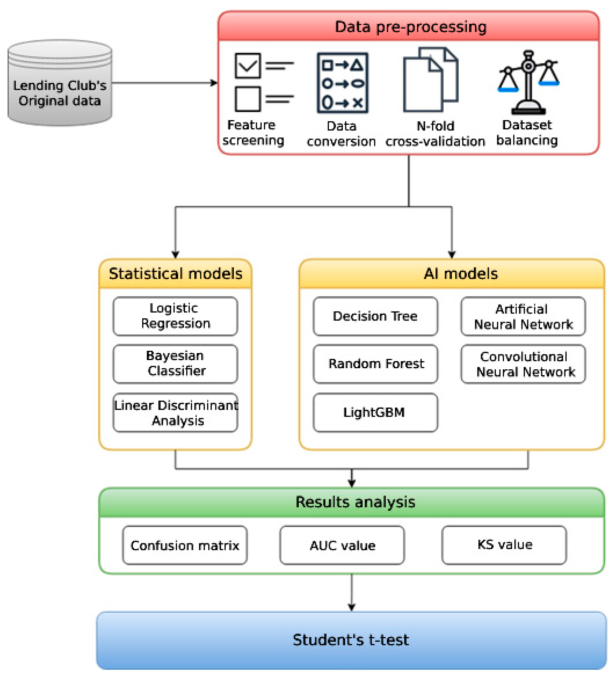
3. Research Process
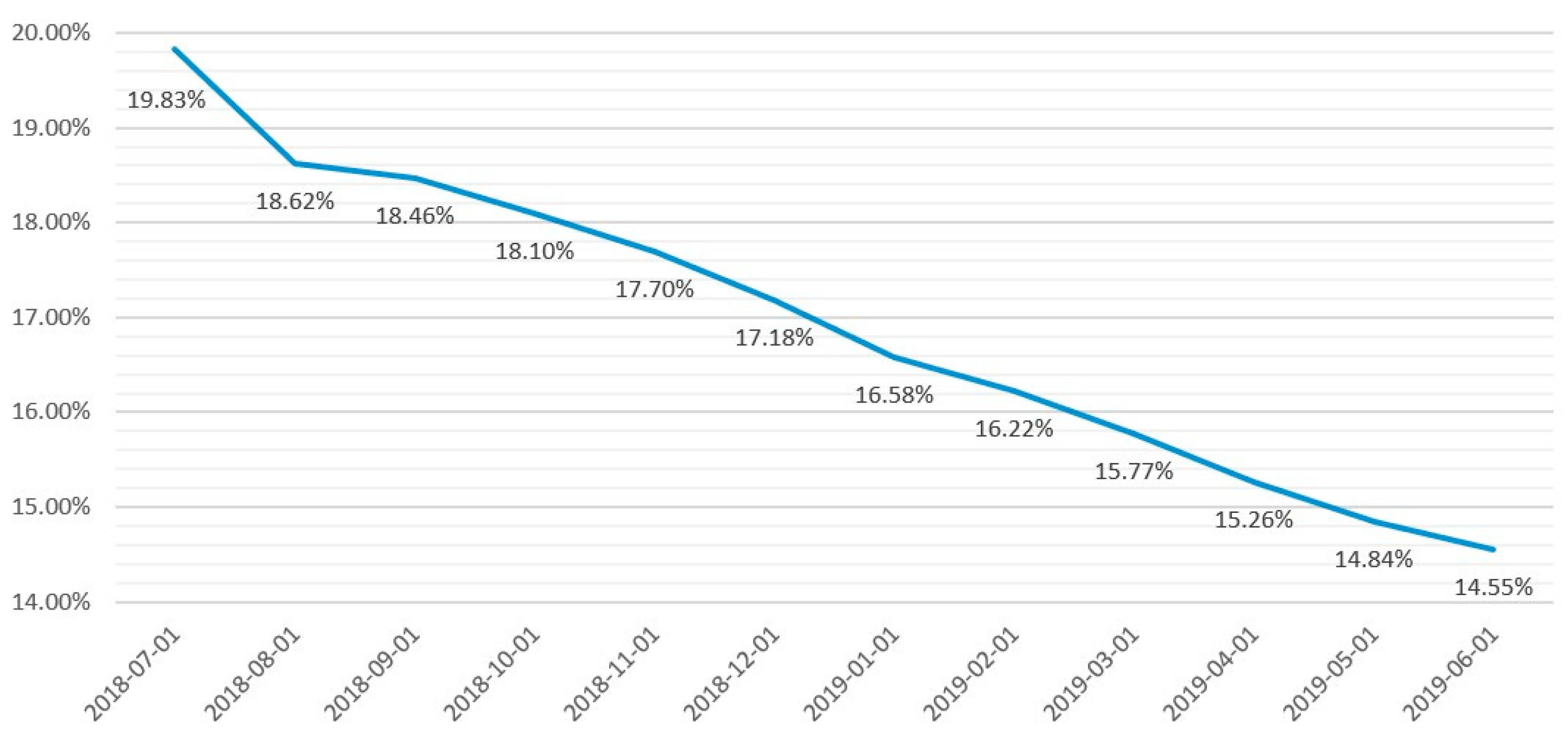
4. Research Data
4.1. Feature Screening
4.2. Data Conversion
- Nominal data: On a nominal scale, events or objects are divided into distinct categories without considering order or ranking. Instead, these categories are given unique labels, and calculations for adding, subtracting, multiplying, and dividing the nominal scales are meaningless. Therefore, this study converts nominal-scale variables into the quantitative scale to feed into the model.
- Ordinal data: The ordinal scale represents the hierarchical relationship among levels on a scale. However, it cannot measure the distance between different levels. This paper converts ordinal data such as debt level, duration of the loan, etc., into numerical data.
- Numerical data: Most of the data in this research are discrete and not highly correlated; i.e., the degree of mutual influence between customers is low. Therefore, missing data are replaced by the average values. After that, data are scaled in the range 0–1 using min–max normalization as follows:where
- is the normalized value;
- is the minimum value of the series to be normalized;
- is the maximum value of the series to be normalized.
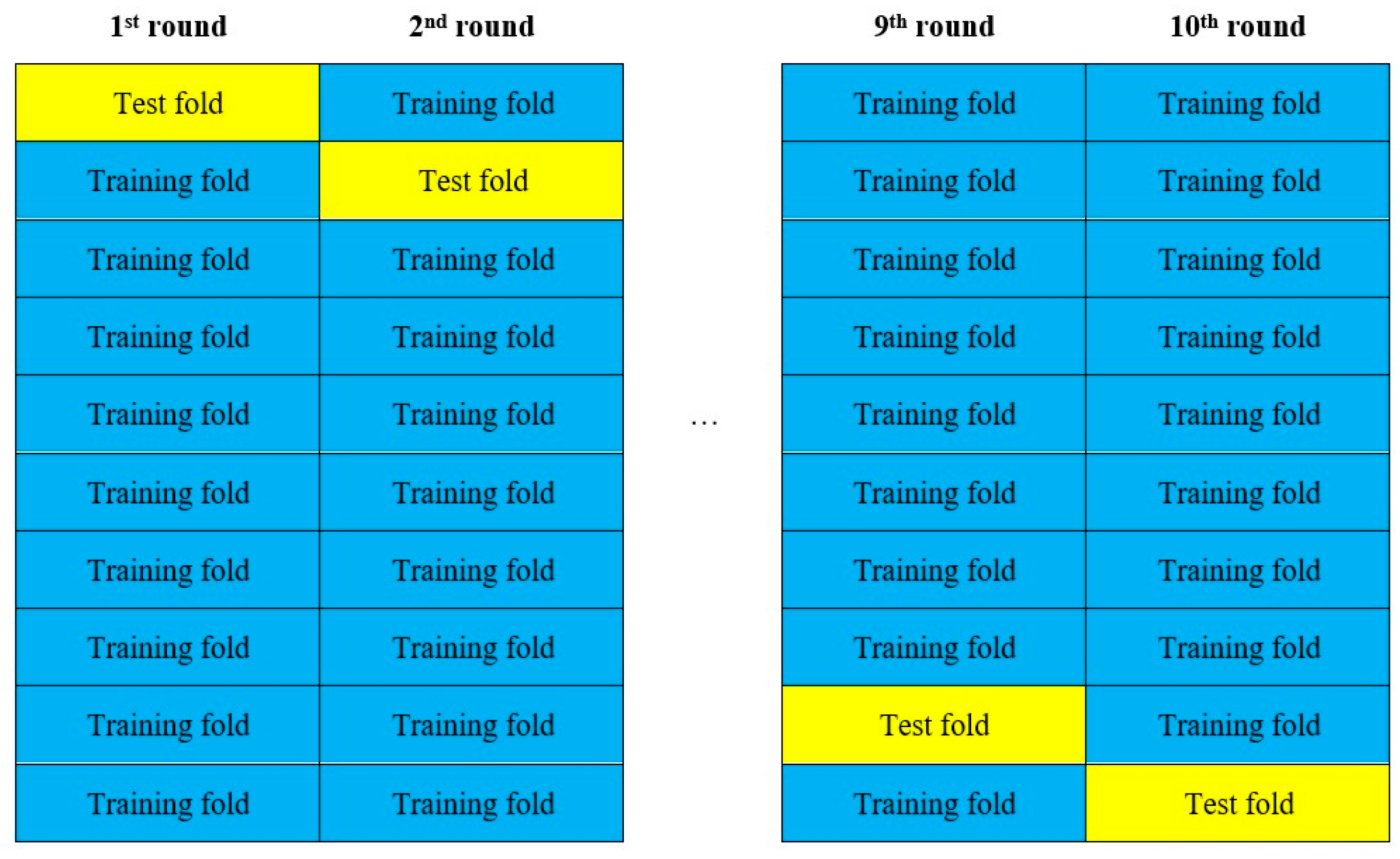
4.3. Ten-Fold Cross-Validation
4.4. Data Balancing
5. Model Construction
5.1. Statistical Models
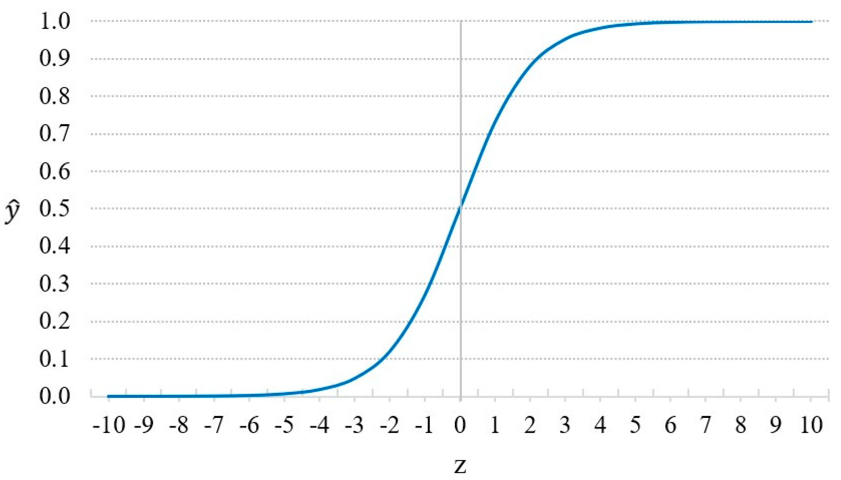
5.1.1. Logistic Regression
- is the input feature vector of the ith instance;
- is the actual observation of the ith instance, ( indicates a default event; indicates a non-default event);
- is the probability of default of the ith instance, given;
- follows the Sigmoid function in Equation (3):where is the constant term; is the regression coefficient).
5.1.2. Bayesian Classifier
- C represents the target (“Fully-Paid” or “Charged-Off” loan);
- represent k features.
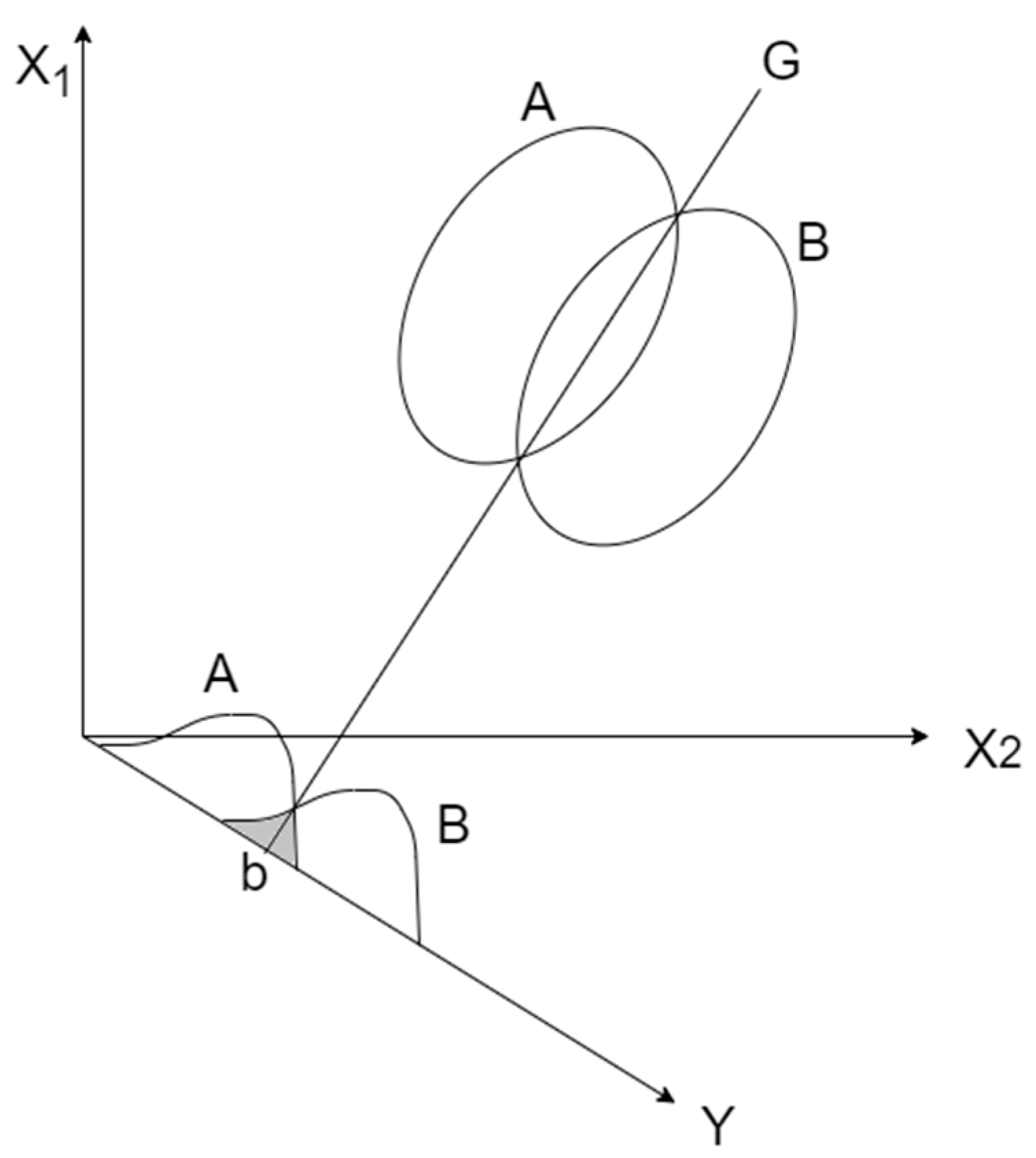
5.1.3. Linear Discriminant Analysis (LDA)
5.2. AI Models
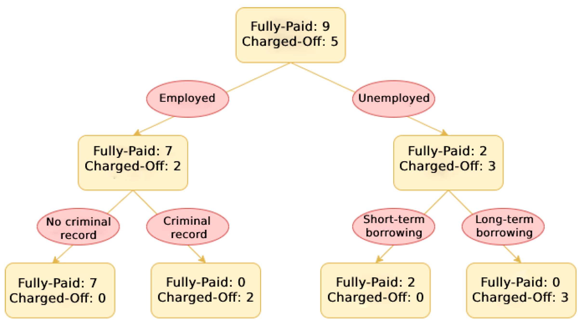
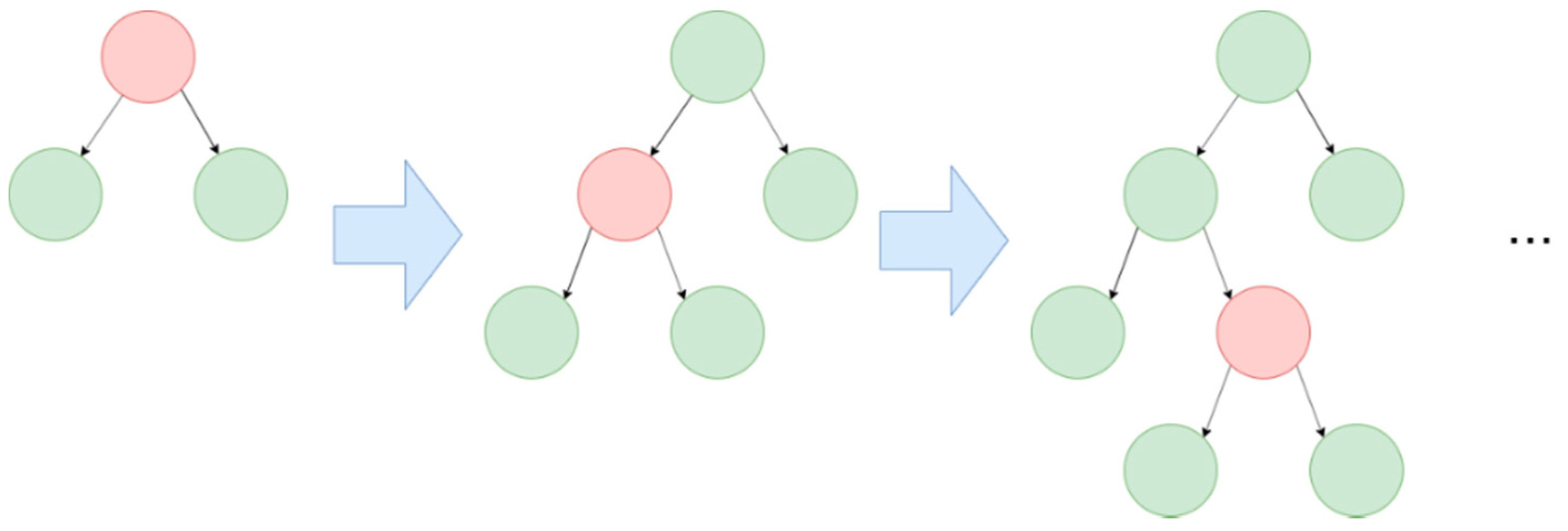
5.2.1. Decision Tree
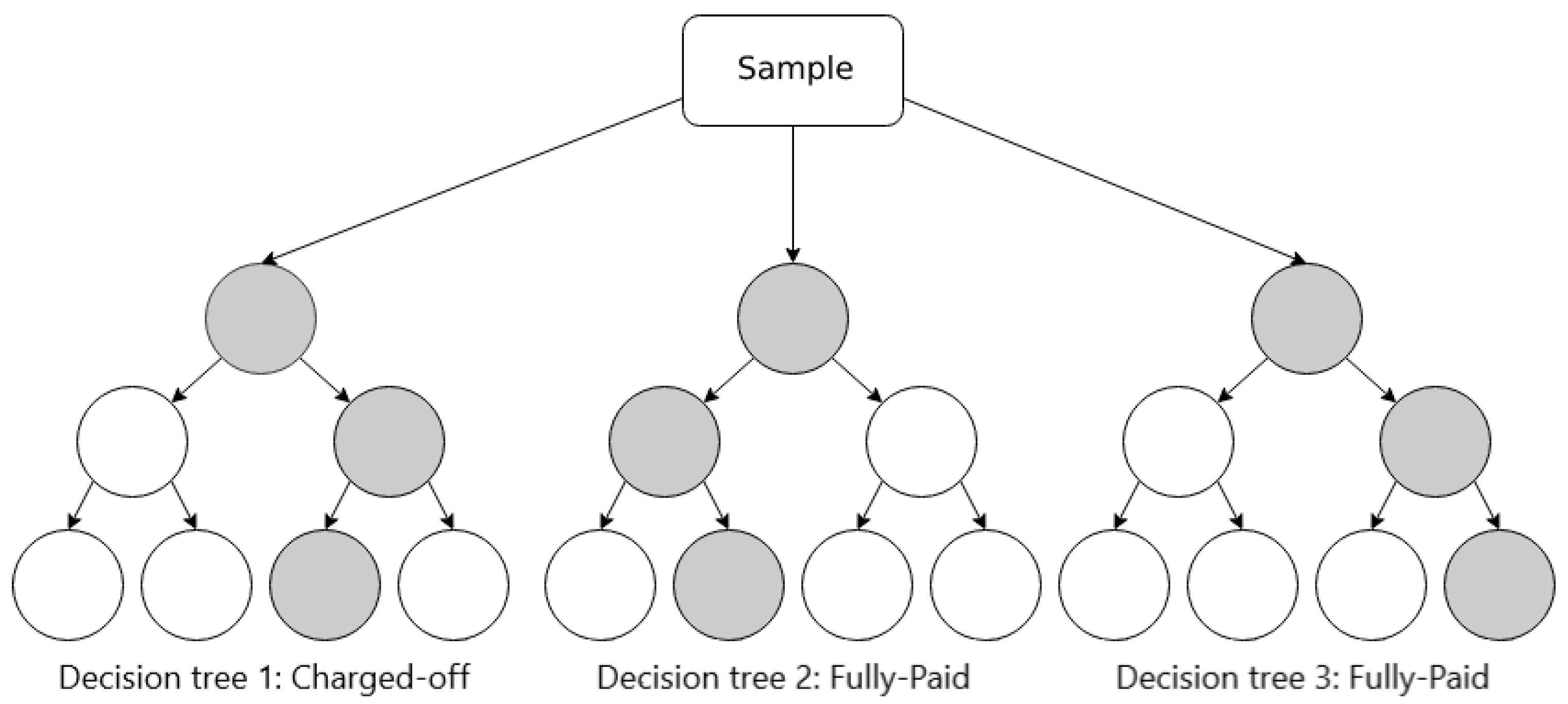
5.2.2. Random Forest
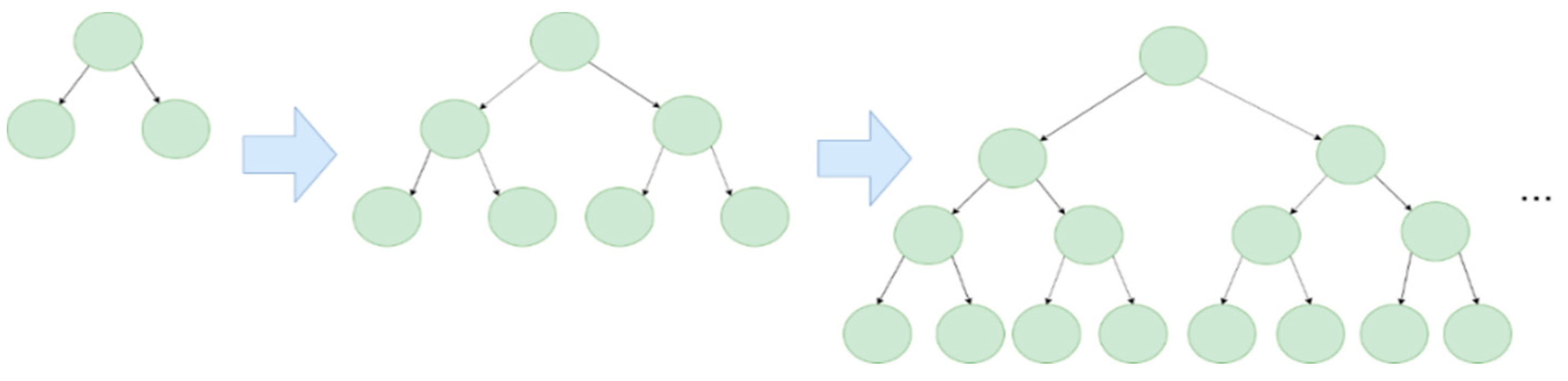
5.2.3. LightGBM
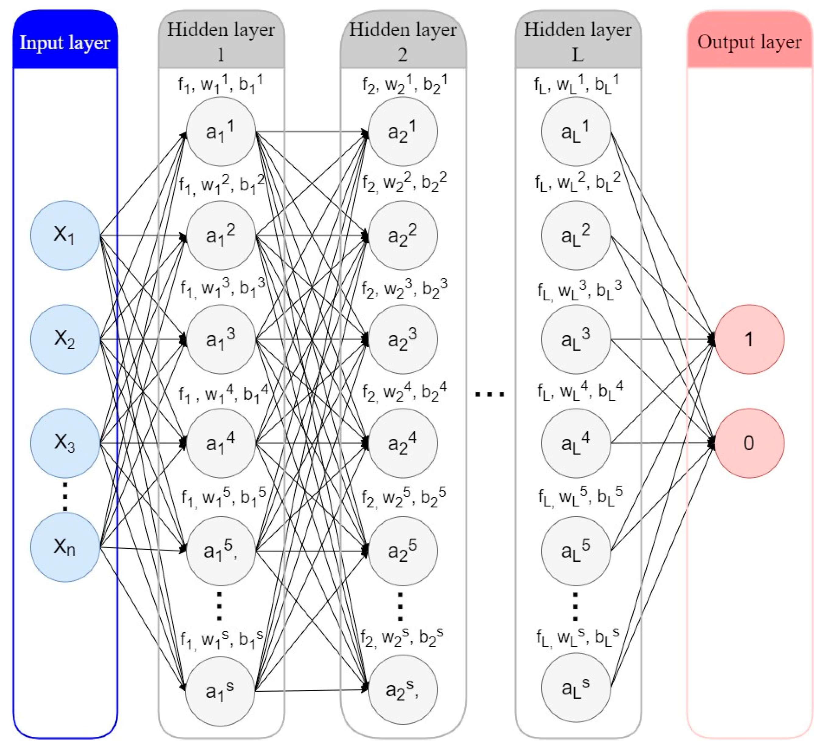
5.2.4. Artificial Neural Network (ANN)
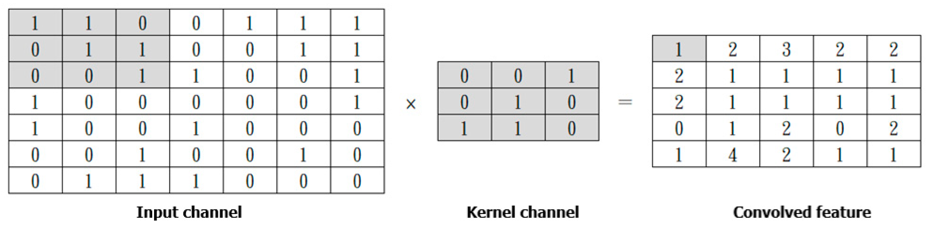
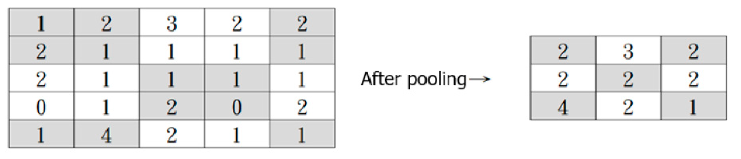
5.2.5. Convolutional Neural Network (CNN)
6. Evaluation Measures
6.1. The Confusion Matrix Series of Metrics
- TP: the number of “Charged-Off” loans correctly predicted;
- FP: the number of “Charged-Off” loans incorrectly predicted (Type I error);
- TN: the number of “Fully-Paid” loans correctly predicted;
- FN: the number of “Fully-Paid” loans incorrectly predicted (Type II error).
6.1.1. Specificity (True Negative Rate—TNR)
6.1.2. Negative Predictive Value (NPV)
6.1.3. Precision (Positive Predictive Value—PPV)
6.1.4. Recall (Sensitivity)
6.1.5. F-Measure
6.1.6. Kappa (Cohen’s Kappa Coefficient)
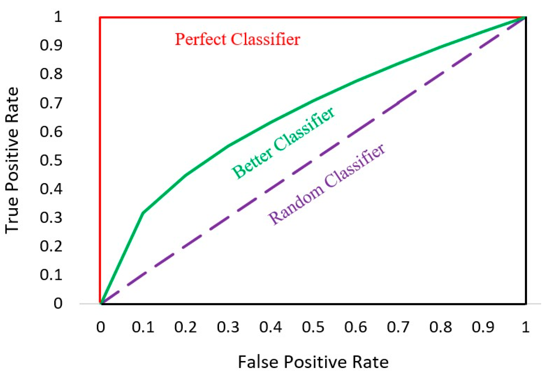
6.2. AUC-ROC Curve
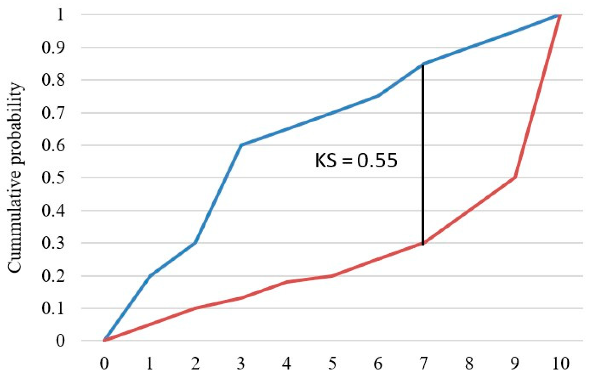
6.3. Kolmogorov–Smirnov Chart (KS)
6.4. Student’s t-Test
- , : The means of the two samples;
- : The difference between the means of the two populations, where is expected to be 0;
- i = 1, 2 … n;
- n: sample size.
7. Results Analysis
8. Discussion and Conclusions
8.1. Discussion
8.2. Conclusions
Author Contributions
Funding
Data Availability Statement
Conflicts of Interest
Appendix A. Detailed Description of Features

| ORDER | FEATURES | DESCRIPTONS |
|---|---|---|
| 1 | acc_open_past_24mths | Number of trades opened in past 24 months. |
| 2 | annual_inc | The self-reported annual income provided by the borrower during registration. |
| 3 | application_type | Indicates whether the loan is an individual application or a joint application with two co-borrowers. |
| 4 | chargeoff_within_12_mths | Number of Charged-Offs within 12 months. |
| 5 | collections_12_mths_ex_med | Number of collections in 12 months excluding medical collections. |
| 6 | delinq_2yrs | The number of 30+ days past-due incidences of delinquency in the borrower’s credit file for the past 2 years. |
| 7 | delinq_amnt | Accounts on which the borrower is now delinquent. |
| 8 | fico_range_high | The upper boundary range that the borrower’s FICO at loan origination belongs to. |
| 9 | fico_range_low | The lower boundary range that the borrower’s FICO at loan origination belongs to. |
| 10 | funded_amnt | The total amount committed to that loan at that point in time. |
| 11 | funded_amnt_inv | The total amount committed by investors to that loan at that point in time. |
| 12 | grade | LC-assigned loan grade. |
| 13 | home_ownership | The home ownership status provided by the borrower during registration or obtained from the credit report. Our values are: RENT, OWN, MORTGAGE, and OTHER. |
| 14 | initial_list_status | The initial listing status of the loan. Possible values are—W, F. |
| 15 | inq_fi | Number of personal finance inquiries. |
| 16 | inq_last_12m | Number of credit inquiries in past 12 months. |
| 17 | inq_last_6mths | The number of inquiries in past 6 months (excluding auto and mortgage inquiries). |
| 18 | installment | The monthly payment owed by the borrower if the loan originates. |
| 19 | int_rate | Interest rate on the loan. |
| 20 | issue_d | The month in which the loan was funded. |
| 21 | loan_amnt | The listed amount of the loan applied for by the borrower. If at some point in time, the credit department reduces the loan amount, then it will be reflected in this value. |
| 22 | max_bal_bc | Maximum current balance owed on all revolving accounts. |
| 23 | mo_sin_old_rev_tl_op | Months since oldest revolving account opened. |
| 24 | mo_sin_rcnt_rev_tl_op | Months since most recent revolving account opened. |
| 25 | mo_sin_rcnt_tl | Months since most recent account opened. |
| 26 | mort_acc | Number of mortgage accounts. |
| 27 | num_accts_ever_120_pd | Number of accounts ever 120 or more days past due. |
| 28 | num_actv_bc_tl | Number of currently active bankcard accounts. |
| 29 | num_actv_rev_tl | Number of currently active revolving trades. |
| 30 | num_bc_sats | Number of satisfactory bankcard accounts. |
| 31 | num_bc_tl | Number of bankcard accounts. |
| 32 | num_il_tl | Number of installment accounts. |
| 33 | num_op_rev_tl | Number of open revolving accounts. |
| 34 | num_rev_accts | Number of revolving accounts. |
| 35 | num_rev_tl_bal_gt_0 | Number of revolving trades with balance >0. |
| 36 | num_sats | Number of satisfactory accounts. |
| 37 | num_tl_90g_dpd_24m | Number of accounts 90 or more days past due in last 24 months. |
| 38 | num_tl_op_past_12m | Number of accounts opened in past 12 months. |
| 39 | open_acc | The number of open credit lines in the borrower’s credit file. |
| 40 | open_acc_6m | Number of open trades in last 6 months. |
| 41 | open_act_il | Number of currently active installment trades. |
| 42 | open_il_12m | Number of installment accounts opened in past 12 months. |
| 43 | open_il_24m | Number of installment accounts opened in past 24 months. |
| 44 | open_rv_12m | Number of revolving trades opened in past 12 months. |
| 45 | open_rv_24m | Number of revolving trades opened in past 24 months. |
| 46 | pct_tl_nvr_dlq | Percent of trades never delinquent. |
| 47 | pub_rec | Number of derogatory public records. |
| 48 | pub_rec_bankruptcies | Number of public record bankruptcies. |
| 49 | purpose | A category provided by the borrower for the loan request. |
| 50 | revol_bal | Total credit revolving balance. |
| 51 | term | The number of payments on the loan. Values are in months and can be either 36 or 60. |
| 52 | title | The loan title provided by the borrower. |
| 53 | tot_coll_amt | Total collection amounts ever owed. |
| 54 | tot_cur_bal | Total current balance of all accounts. |
| 55 | tot_hi_cred_lim | Total high credit/credit limit. |
| 56 | total_acc | The total number of credit lines currently in the borrower’s credit file. |
| 57 | total_bal_ex_mort | Total credit balance excluding mortgage. |
| 58 | total_bal_il | Total current balance of all installment accounts. |
| 59 | total_bc_limit | Total bankcard high credit/credit limit. |
| 60 | total_cu_tl | Number of finance trades. |
| 61 | total_il_high_credit_limit | Total installment high credit/credit limit. |
| 62 | total_rev_hi_lim | Total revolving high credit/credit limit. |
| 63 | verification_status | Indicates if income was verified by LC, not verified, or if the income source was verified. |
Appendix B. Model’s p-Values for Each Metric
| Bayesian Classifier | CNN | Random Forest | LDA | LightGBM | Logistic Regression | ANN | Decision Tree | |
|---|---|---|---|---|---|---|---|---|
| Bayesian Classifier | 1.0000 | |||||||
| CNN | 0.0000 *** | 1.0000 | ||||||
| Random Forest | 0.2521 | 0.0000 *** | 1.0000 | |||||
| LDA | 0.0000 *** | 0.1008 | 0.0000 *** | 1.0000 | ||||
| LightGBM | 0.0000 *** | 0.0110 ** | 0.0000 *** | 0.0001 *** | 1.0000 | |||
| Logistic Regression | 0.0000 *** | 0.1115 | 0.0000 *** | 0.8963 | 0.0001 *** | 1.0000 | ||
| ANN | 0.0000 *** | 0.8995 | 0.0000 *** | 0.0627 * | 0.0103 ** | 0.0684 * | 1.0000 | |
| Decision Tree | 0.0000 *** | 0.0000 *** | 0.0000 *** | 0.0000 *** | 0.0000 *** | 0.0000 *** | 0.0000 *** | 1.0000 |
| Bayesian Classifier | CNN | Random Forest | LDA | LightGBM | Logistic Regression | ANN | Decision Tree | |
|---|---|---|---|---|---|---|---|---|
| Bayesian Classifier | 1.0000 | |||||||
| CNN | 0.0000 *** | 1.0000 | ||||||
| Random Forest | 0.0596 * | 0.0000 *** | 1.0000 | |||||
| LDA | 0.0000 *** | 0.2967 | 0.0000 *** | 1.0000 | ||||
| LightGBM | 0.0000 *** | 0.0046 *** | 0.0000 *** | 0.0002 *** | 1.0000 | |||
| Logistic Regression | 0.0000 *** | 0.3013 | 0.0000 *** | 0.9358 | 0.0001 *** | 1.0000 | ||
| ANN | 0.0000 *** | 0.6565 | 0.0000 *** | 0.1491 | 0.0175 ** | 0.1459 | 1.0000 | |
| Decision Tree | 0.0176 ** | 0.0000 *** | 0.3528 | 0.0000 *** | 0.0000 *** | 0.0000 *** | 0.0000 *** | 1.0000 |
| Bayesian Classifier | CNN | Random Forest | LDA | LightGBM | Logistic Regression | ANN | Decision Tree | |
|---|---|---|---|---|---|---|---|---|
| Bayesian Classifier | 1.0000 | |||||||
| CNN | 0.0000 *** | 1.0000 | ||||||
| Random Forest | 0.5197 | 0.0000 *** | 1.0000 | |||||
| LDA | 0.0000 *** | 0.2096 | 0.0000 *** | 1.0000 | ||||
| LightGBM | 0.0000 *** | 0.2349 | 0.0000 *** | 0.0002 *** | 1.0000 | |||
| Logistic Regression | 0.0000 *** | 0.1868 | 0.0000 *** | 0.9341 | 0.0001 *** | 1.0000 | ||
| ANN | 0.0000 *** | 0.9130 | 0.0000 *** | 0.3059 | 0.2236 | 0.2803 | 1.0000 | |
| Decision Tree | 0.0000 *** | 0.2980 | 0.0000 *** | 0.8565 | 0.0027 *** | 0.8007 | 0.3979 | 1.0000 |
| Bayesian Classifier | CNN | Random Forest | LDA | LightGBM | Logistic Regression | ANN | Decision Tree | |
|---|---|---|---|---|---|---|---|---|
| Bayesian Classifier | 1.0000 | |||||||
| CNN | 0.4795 | 1.0000 | ||||||
| Random Forest | 0.1473 | 0.3456 | 1.0000 | |||||
| LDA | 0.5267 | 0.9475 | 0.3309 | 1.0000 | ||||
| LightGBM | 0.5254 | 0.0974 * | 0.0169 ** | 0.1282 | 1.0000 | |||
| Logistic Regression | 0.6185 | 0.8117 | 0.2553 | 0.8688 | 0.1677 | 1.0000 | ||
| ANN | 0.4093 | 0.7425 | 0.7113 | 0.7125 | 0.1555 | 0.6241 | 1.0000 | |
| Decision Tree | 0.0000 *** | 0.0000 *** | 0.0002 *** | 0.0000 *** | 0.0000 *** | 0.0000 *** | 0.0010 *** | 1.0000 |
| Bayesian Classifier | CNN | Random Forest | LDA | LightGBM | Logistic Regression | ANN | Decision Tree | |
|---|---|---|---|---|---|---|---|---|
| Bayesian Classifier | 1.0000 | |||||||
| CNN | 0.0029 *** | 1.0000 | ||||||
| Random Forest | 0.2565 | 0.0023 *** | 1.0000 | |||||
| LDA | 0.0021 *** | 0.3997 | 0.0000 *** | 1.0000 | ||||
| LightGBM | 0.0008 *** | 0.6293 | 0.0000 *** | 0.4186 | 1.0000 | |||
| Logistic Regression | 0.0026 *** | 0.3261 | 0.0001 *** | 0.7801 | 0.2542 | 1.0000 | ||
| ANN | 0.0045 *** | 0.8472 | 0.0062 *** | 0.3614 | 0.5326 | 0.3057 | 1.0000 | |
| Decision Tree | 0.0000 *** | 0.0027 *** | 0.0000 *** | 0.0000 *** | 0.0000 *** | 0.0000 *** | 0.0182 ** | 1.0000 |
| Bayesian Classifier | CNN | Random Forest | LDA | LightGBM | Logistic Regression | ANN | Decision Tree | |
|---|---|---|---|---|---|---|---|---|
| Bayesian Classifier | 1.0000 | |||||||
| CNN | 0.0000 *** | 1.0000 | ||||||
| Random Forest | 0.8778 | 0.0000 *** | 1.0000 | |||||
| LDA | 0.0000 *** | 0.1339 | 0.0000 *** | 1.0000 | ||||
| LightGBM | 0.0000 *** | 0.0469 ** | 0.0000 *** | 0.0003 *** | 1.0000 | |||
| Logistic Regression | 0.0000 *** | 0.1155 | 0.0000 *** | 0.9848 | 0.0001 *** | 1.0000 | ||
| ANN | 0.0000 *** | 0.7368 | 0.0000 *** | 0.3504 | 0.0467 ** | 0.3366 | 1.0000 | |
| Decision Tree | 0.0089 *** | 0.0006 *** | 0.0011 *** | 0.0083 *** | 0.0000 *** | 0.0050 *** | 0.0048 *** | 1.0000 |
| Bayesian Classifier | CNN | Random Forest | LDA | LightGBM | Logistic Regression | ANN | Decision Tree | |
|---|---|---|---|---|---|---|---|---|
| Bayesian Classifier | 1.0000 | |||||||
| CNN | 0.6439 | 1.0000 | ||||||
| Random Forest | 0.2736 | 0.5760 | 1.0000 | |||||
| LDA | 0.7704 | 0.7901 | 0.2724 | 1.0000 | ||||
| LightGBM | 0.2350 | 0.0812 * | 0.0025 *** | 0.0395 ** | 1.0000 | |||
| Logistic Regression | 0.8865 | 0.6531 | 0.1487 | 0.8115 | 0.0347 ** | 1.0000 | ||
| ANN | 0.3506 | 0.6048 | 0.9170 | 0.4036 | 0.0354 ** | 0.3093 | 1.0000 | |
| Decision Tree | 0.0000 *** | 0.0000 *** | 0.0000 *** | 0.0000 *** | 0.0000 *** | 0.0000 *** | 0.0001 *** | 1.0000 |
| Bayesian Classifier | CNN | Random Forest | LDA | LightGBM | Logistic Regression | ANN | Decision Tree | |
|---|---|---|---|---|---|---|---|---|
| Bayesian Classifier | 1.0000 | |||||||
| CNN | 0.0000 *** | 1.0000 | ||||||
| Random Forest | 0.4293 | 0.0000 *** | 1.0000 | |||||
| LDA | 0.0001 *** | 0.3739 | 0.0000 *** | 1.0000 | ||||
| LightGBM | 0.0000 *** | 0.0029 *** | 0.0000 *** | 0.0011 *** | 1.0000 | |||
| Logistic Regression | 0.0000 *** | 0.3938 | 0.0000 *** | 0.8992 | 0.0005 *** | 1.0000 | ||
| ANN | 0.0000 *** | 0.4040 | 0.0000 *** | 0.8964 | 0.0006 *** | 0.9956 | 1.0000 | |
| Decision Tree | 0.2596 | 0.0000 *** | 0.6309 | 0.0000 *** | 0.0000 *** | 0.0000 *** | 0.0000 *** | 1.0000 |
Appendix C. AI Model’s Parameters
| MODEL | PARAMETERS | VALUES |
|---|---|---|
| Decision Tree | Criterion | ‘gini’ |
| Splitter | ‘best’ | |
| Min_samples_leaf | 1 | |
| RandomForest | Criterion | entropy |
| N_estimators | 10 | |
| N_jobs | 1 | |
| CNN | Conv1D[filters, kernel_size, activation, input_shape] | [64, 3, sigmoid, 63] |
| MaxPooling1D | 2 | |
| Conv1D[filters, kernel_size, activation] | [64, 3, sigmoid] | |
| MaxPooling1D | 2 | |
| Conv1D[filters, kernel_size, activation] | [64, 3, sigmoid] | |
| Flatten | ||
| Dense[units, activation] | [64, sigmoid] | |
| Dense[units, activation] | [1, sigmoid] | |
| Optimizer | adam | |
| Loss | binary_crossentropy | |
| Epochs | 1000 | |
| Batch_size | 2000 | |
| ANN | Dense[units, activation] | [63, sigmoid] |
| Dense[units, activation] | [25, sigmoid] | |
| Dense[units, activation] | [50, sigmoid] | |
| Dense[units, activation] | [100, sigmoid] | |
| Dense[units, activation] | [50, sigmoid] | |
| Dense[units, activation] | [25, sigmoid] | |
| Dense[units, activation] | [1, sigmoid] | |
| Optimizer | adam | |
| Loss | binary_crossentropy | |
| Epochs | 5000 | |
| Batch_size | 2000 | |
| LightGBM | Learning_rate | 0.01 |
| Max_depth | −1 | |
| Num_iteration | 300 | |
| Objective | binary |
References
- Lenz, R. Peer-to-peer lending: Opportunities and risks. Eur. J. Risk Regul. 2016, 7, 688–700. [Google Scholar] [CrossRef]
- Chen, S.; Yan, G.; Qingfu, L.; Yiuman, T. How do lenders evaluate borrowers in peer-to-peer lending in China? Int. Rev. Econ. Financ. 2020, 69, 651–662. [Google Scholar] [CrossRef]
- Jiang, J.; Liao, L.; Wang, Z.; Zhang, X. Government affiliation and peer-to-peer lending platforms in China. J. Empir. Financ. 2021, 62, 87–106. [Google Scholar] [CrossRef]
- He, Q.; Li, X. The failure of Chinese peer-to-peer lending platforms: Finance and politics. J. Corp. Financ. 2021, 66, 101852. [Google Scholar] [CrossRef]
- Tsai, C.-H. To regulate or not to regulate: A comparison of government responses to peer-to-peer lending among the United States, China, and Taiwan. U. Cin. L. Rev. 2018, 87, 1077. [Google Scholar]
- Big Data, Big Impact: New Possibilities for International Development. Available online: https://www.weforum.org/reports/big-data-big-impact-new-possibilities-international-development (accessed on 30 October 2021).
- Cao, X. Risk management and control countermeasures of P2P network lending platform under internet financial environment. In Proceedings of the 2nd International Conference on Global Economy, Finance and Humanities Research, Tianjin, China, 15–16 June 2019. [Google Scholar]
- Teply, P.; Polena, M. Best classification algorithms in peer-to-peer lending. North Am. J. Econ. Financ. 2020, 51, 100904. [Google Scholar] [CrossRef]
- Malekipirbazari, M.; Aksakalli, V. Risk assessment in social lending via random forests. Expert Syst. Appl. 2015, 42, 4621–4631. [Google Scholar] [CrossRef]
- Reddy, S.; Gopalaraman, K. Peer to peer lending, default prediction-evidence from lending club. J. Internet Bank. Commer. 2016, 21, 211. [Google Scholar]
- Ma, X.; Sha, J.; Wang, D.; Yu, Y.; Yang, Q.; Niu, X. Study on a prediction of P2P network loan default based on the machine learning LightGBM and XGboost algorithms according to different high dimensional data cleaning. Electron. Commer. Res. Appl. 2018, 31, 24–39. [Google Scholar] [CrossRef]
- Duan, J. Financial system modeling using deep neural networks (DNNs) for effective risk assessment and prediction. J. Frankl. Inst. 2019, 356, 4716–4731. [Google Scholar] [CrossRef]
- Babaei, G.; Bamdad, S. A multi-objective instance-based decision support system for investment recommendation in peer-to-peer lending. Expert Syst. Appl. 2020, 150, 113278. [Google Scholar] [CrossRef]
- Kim, J.-Y.; Cho, S.-B. Deep dense convolutional networks for repayment prediction in peer-to-peer lending. In Proceedings of the 13th International Conference on Soft Computing Models in Industrial and Environmental Applications, San Sebastián, Spain, 6–8 June 2018. [Google Scholar]
- Ha, V.-S.; Lu, D.-N.; Choi, G.S.; Nguyen, H.-N.; Yoon, B. Improving credit risk prediction in online peer-to-peer (P2P) lending using feature selection with deep learning. In Proceedings of the 2019 21st International Conference on Advanced Communication Technology (ICACT), PyeongChang, Korea, 17–20 February 2019. [Google Scholar]
- Ferreira, L.E.B.; Barddal, J.P.; Gomes, H.M.; Enembreck, F. Improving credit risk prediction in online peer-to-peer (P2P) lending using imbalanced learning techniques. In Proceedings of the 2017 IEEE 29th International Conference on Tools with Artificial Intelligence (ICTAI), Boston, MA, USA, 6–8 November 2017. [Google Scholar]
- Xia, Y. A novel reject inference model using outlier detection and gradient boosting technique in peer-to-peer lending. IEEE Access 2019, 7, 92893–92907. [Google Scholar] [CrossRef]
- Zhang, Y.; Li, H.; Hai, M.; Li, J.; Li, A. Determinants of loan funded successful in online P2P Lending. Procedia Comput. Sci. 2017, 122, 896–901. [Google Scholar] [CrossRef]
- Vedala, R.; Kumar, B.P. An application of naive bayes classification for credit scoring in e-lending platform. In Proceedings of the 2012 International Conference on Data Science & Engineering (ICDSE), Cochin, India, 18–20 July 2012. [Google Scholar]
- Luo, B.; Lin, Z. A decision tree model for herd behavior and empirical evidence from the online P2P lending market. Inf. Syst. E-Bus. Manag. 2013, 11, 141–160. [Google Scholar] [CrossRef]
- Kohavi, R. A study of cross-validation and bootstrap for accuracy estimation and model selection. In Proceedings of the 1995 International Joint Conference on AI (IJCAI), Montreal, QC, Canada, 20–25 August 1995. [Google Scholar]
- Fisher, R.A. The use of multiple measurements in taxonomic problems. Ann. Eugen. 1936, 7, 179–188. [Google Scholar] [CrossRef]
- LeCun, Y.; Bottou, L.; Bengio, Y.; Haffner, P. Gradient-based learning applied to document recognition. Proc. IEEE 1998, 86, 2278–2324. [Google Scholar] [CrossRef] [Green Version]
- Cohen, J. A coefficient of agreement for nominal scales. Educ. Psychol. Meas. 1960, 20, 37–46. [Google Scholar] [CrossRef]
- Landis, J.R.; Koch, G.G. The measurement of observer agreement for categorical data. Biometrics 1977, 33, 159–174. [Google Scholar] [CrossRef] [PubMed] [Green Version]
- Student. The probable error of a mean. Biometrika 1908, 6, 1–25. [Google Scholar] [CrossRef]
- LendingClub Reports Fourth Quarter and Full Year 2021 Results. Available online: https://ir.lendingclub.com/news/news-details/2022/LendingClub-Reports-Fourth-Quarter-and-Full-Year-2021-Results/default.aspx (accessed on 31 March 2022).


| Loan Status | Quantity | Proportion |
|---|---|---|
| Fully-Paid | 52,117 | 85.45% |
| Charged-Off | 8876 | 14.55% |
| Total | 60,993 | 100% |
| Actual “Charged-Off” | Actual “Fully-Paid” | |
|---|---|---|
| Predicted “Charged-Off” | True Positive (TP) | False Positive (FP) Type I error |
| Predicted “Fully-Paid” | False Negative (FN) Type II error | True Negative (TN) |
| LightGBM | CNN | Logistic Regression | LDA | ANN | Bayesian Classifier | Random Forest | Decision Tree | |
|---|---|---|---|---|---|---|---|---|
| Accuracy | 68.57% | 67.27% | 66.87% | 66.81% | 66.85% | 64.27% | 63.89% | 63.63% |
| AUC value | 74.92% | 73.56% | 72.82% | 72.76% | 73.63% | 68.58% | 69.06% | 65.59% |
| KS value | 38.37% | 35.81% | 34.97% | 34.90% | 36.22% | 30.49% | 28.93% | 27.93% |
| Specificity | 71.47% | 69.53% | 67.32% | 67.40% | 69.28% | 56.41% | 57.56% | 67.62% |
| NPV | 67.55% | 66.58% | 66.73% | 66.62% | 66.28% | 67.11% | 65.92% | 62.60% |
| Recall | 65.66% | 64.94% | 66.44% | 66.23% | 64.50% | 72.16% | 70.23% | 59.62% |
| Precision | 69.73% | 68.24% | 67.05% | 67.03% | 67.91% | 62.44% | 62.33% | 64.87% |
| F-measure | 67.62% | 66.43% | 66.72% | 66.61% | 65.95% | 66.82% | 66.04% | 62.11% |
| Kappa | 37.13% | 34.49% | 33.75% | 33.62% | 33.75% | 28.56% | 27.79% | 27.24% |
| LightGBM | CNN | Logistic Regression | LDA | ANN | Bayesian Classifier | Random Forest | Decision Tree | |
|---|---|---|---|---|---|---|---|---|
| LightGBM | 1.0000 | |||||||
| CNN | 0.0034 *** | 1.0000 | ||||||
| Logistic Regression | 0.0005 *** | 0.3593 | 1.0000 | |||||
| LDA | 0.0012 *** | 0.3450 | 0.9011 | 1.0000 | ||||
| ANN | 0.0006 *** | 0.3425 | 0.9606 | 0.9378 | 1.0000 | |||
| Bayesian Classifier | 0.0000 *** | 0.0000 *** | 0.0000 *** | 0.0001 *** | 0.0000 *** | 1.0000 | ||
| Random Forest | 0.0000 *** | 0.0000 *** | 0.0000 *** | 0.0000 *** | 0.0000 *** | 0.4524 | 1.0000 | |
| Decision Tree | 0.0000 *** | 0.0000 *** | 0.0000 *** | 0.0000 *** | 0.0000 *** | 0.2859 | 0.6431 | 1.0000 |
| LightGBM | CNN | Logistic Regression | LDA | ANN | Bayesian Classifier | Random Forest | Decision Tree | |
|---|---|---|---|---|---|---|---|---|
| Accuracy | 68.57% | 67.27% | 66.87% | 66.81% | 66.85% | 64.27% | 63.89% | 63.63% |
| Average: 65.66% | ||||||||
| Difference | 2.91% | |||||||
| LC’s revenue | USD 818,600,000 | |||||||
| Revenue improvement | USD 23,821,260 | |||||||
| The Best Model | Model(s) Have No Significant Difference from the Best Model | |
|---|---|---|
| Accuracy | LightGBM | |
| AUC value | LightGBM | |
| KS value | LightGBM | |
| Specificity | LightGBM | CNN, ANN |
| NPV | LightGBM | Bayesian Classifier, Logistic Regression, LDA, ANN |
| Recall | Bayesian Classifier | Random Forest |
| Precision | LightGBM | |
| F-measure | LightGBM | Bayesian Classifier |
| Kappa | LightGBM |
Publisher’s Note: MDPI stays neutral with regard to jurisdictional claims in published maps and institutional affiliations. |
© 2022 by the authors. Licensee MDPI, Basel, Switzerland. This article is an open access article distributed under the terms and conditions of the Creative Commons Attribution (CC BY) license (https://creativecommons.org/licenses/by/4.0/).
Share and Cite
Ko, P.-C.; Lin, P.-C.; Do, H.-T.; Huang, Y.-F. P2P Lending Default Prediction Based on AI and Statistical Models. Entropy 2022, 24, 801. https://doi.org/10.3390/e24060801
Ko P-C, Lin P-C, Do H-T, Huang Y-F. P2P Lending Default Prediction Based on AI and Statistical Models. Entropy. 2022; 24(6):801. https://doi.org/10.3390/e24060801
Chicago/Turabian StyleKo, Po-Chang, Ping-Chen Lin, Hoang-Thu Do, and You-Fu Huang. 2022. "P2P Lending Default Prediction Based on AI and Statistical Models" Entropy 24, no. 6: 801. https://doi.org/10.3390/e24060801