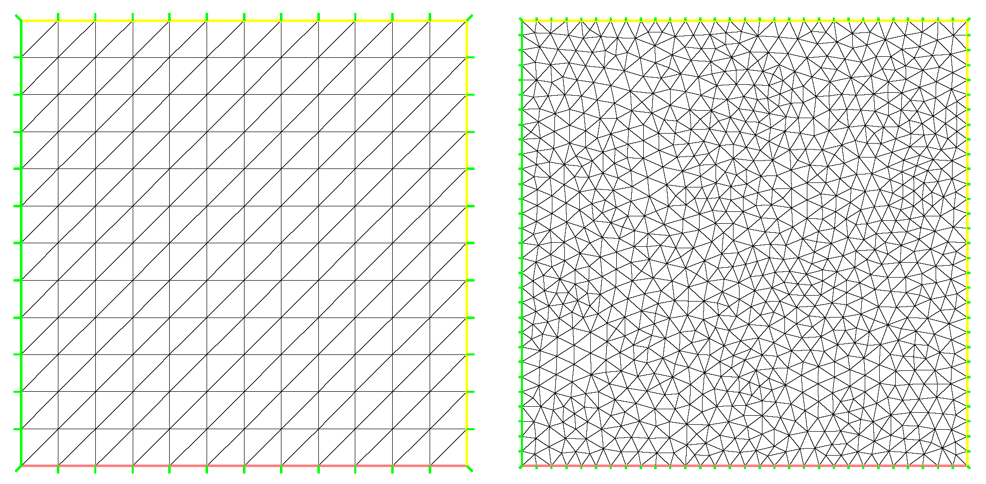
Figure 1.
Two kinds of mesh.
Figure 1.
Two kinds of mesh.
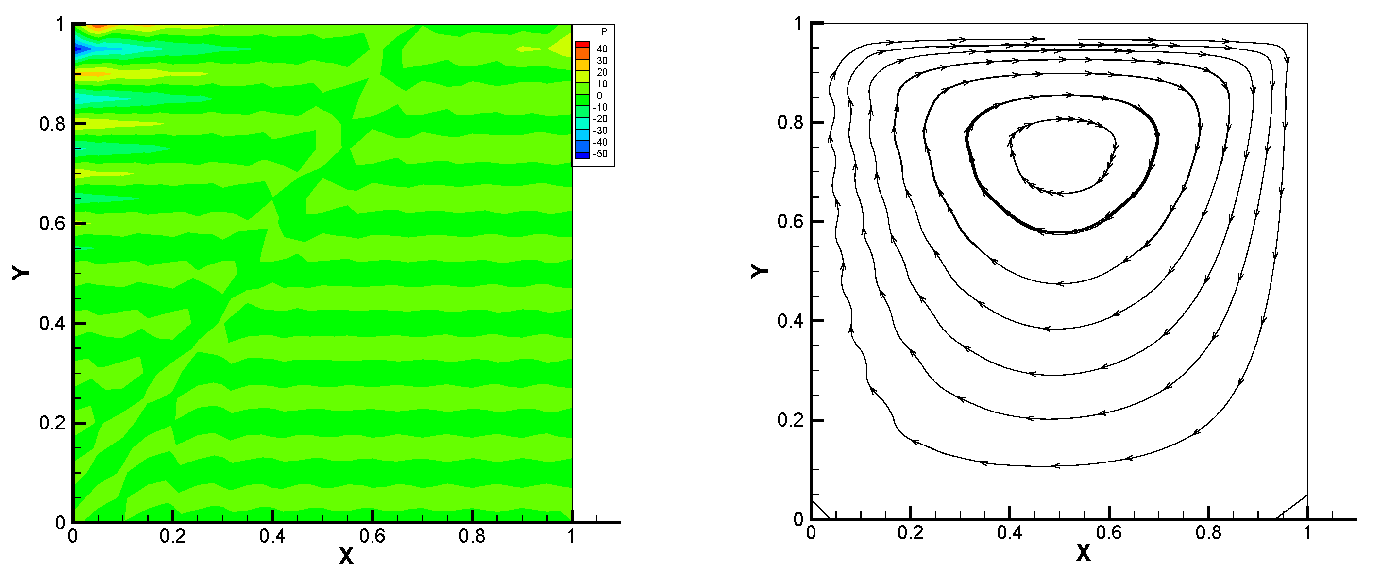
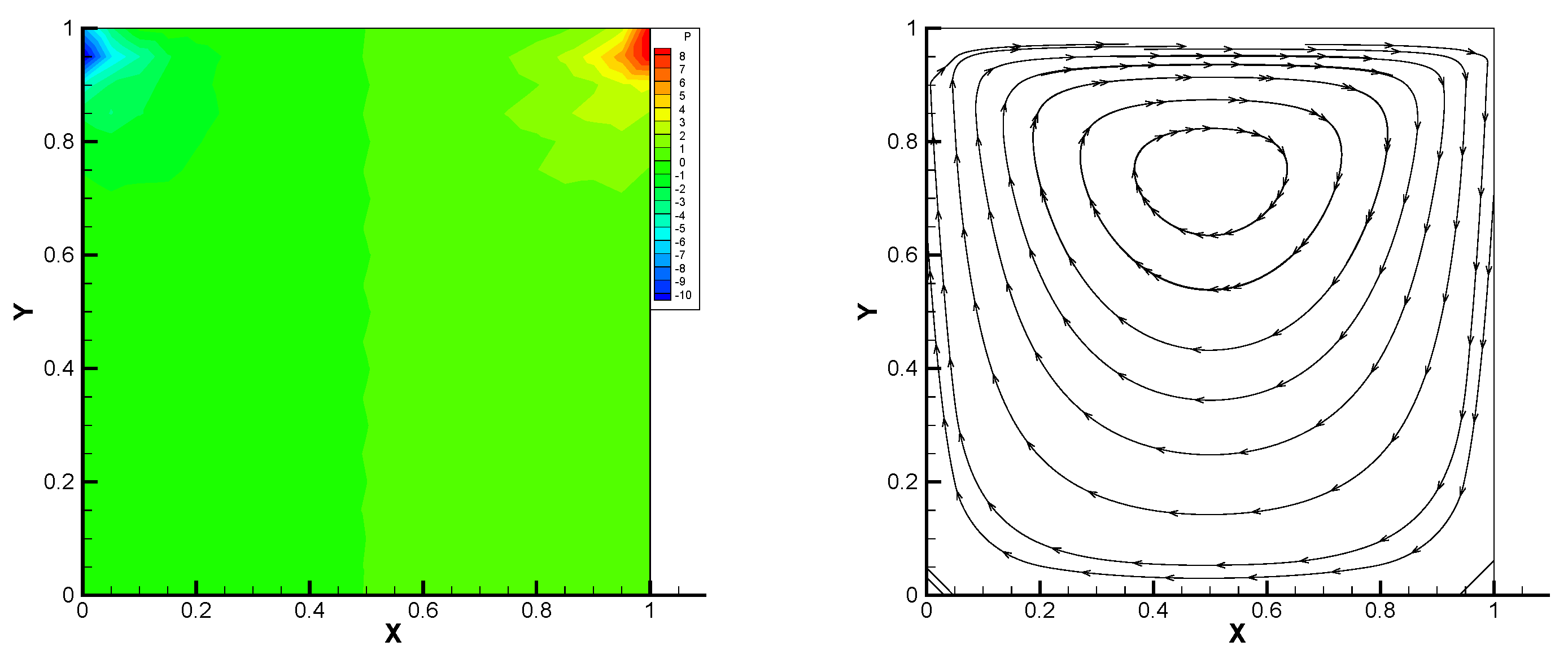
Figure 2.
Pressure level lines and velocity streamlines for the penalty method.
Figure 2.
Pressure level lines and velocity streamlines for the penalty method.
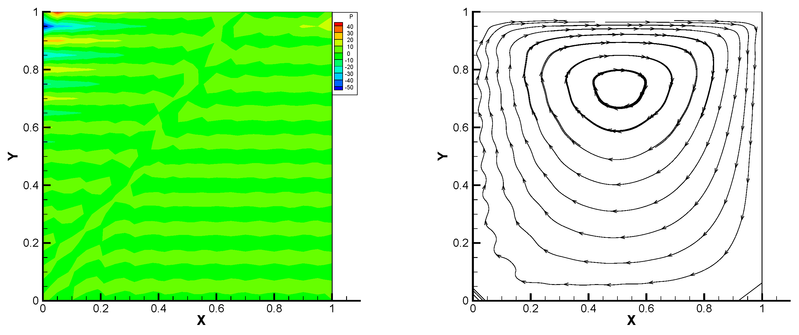
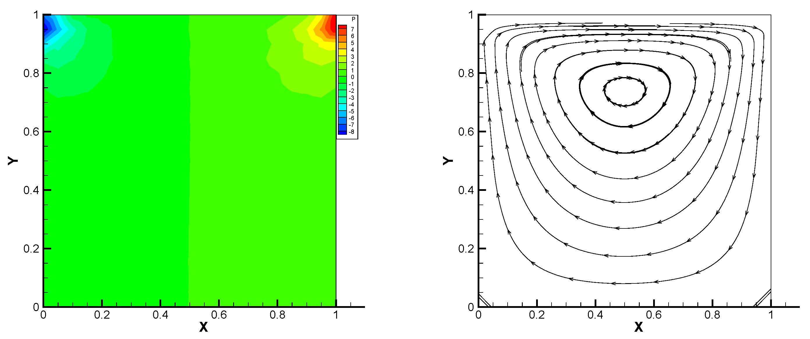
Figure 3.
Pressure level lines and velocity streamlines for the regular method.
Figure 3.
Pressure level lines and velocity streamlines for the regular method.
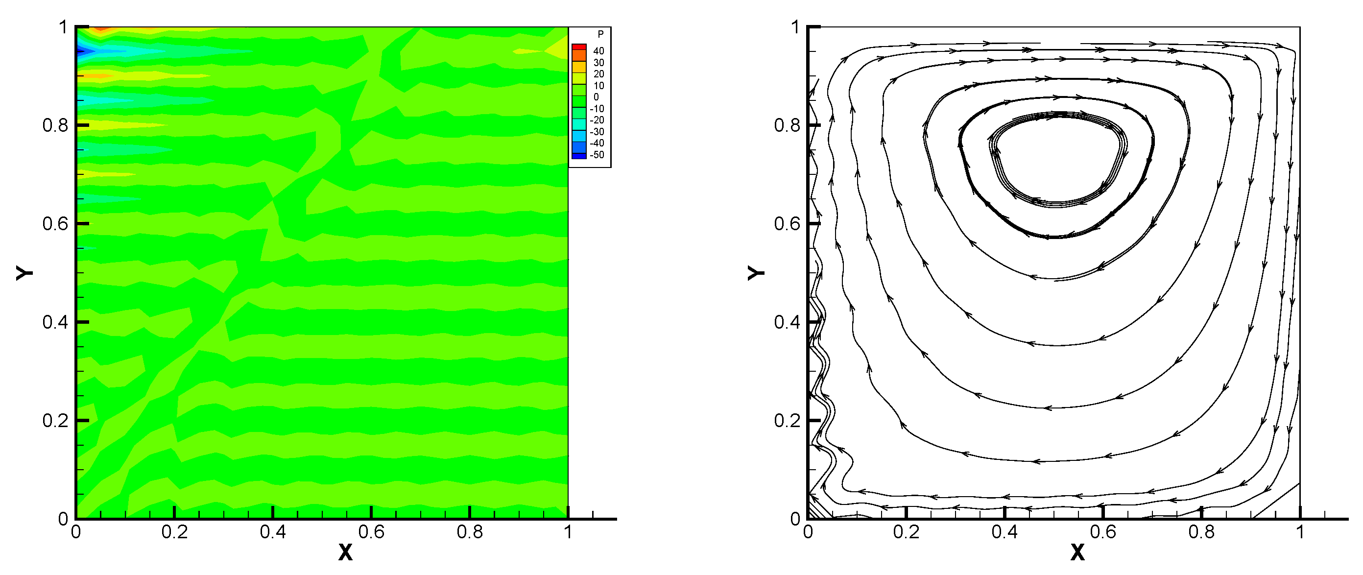
Figure 4.
Pressure level lines and velocity streamlines for the multiscale enrichment method.
Figure 4.
Pressure level lines and velocity streamlines for the multiscale enrichment method.
Figure 5.
Pressure level lines and velocity streamlines for the local Gauss intergration method.
Figure 5.
Pressure level lines and velocity streamlines for the local Gauss intergration method.
Figure 6.
Pressure level lines and velocity streamlines for the local Gauss intergration method of p1b-p1-p1b.
Figure 6.
Pressure level lines and velocity streamlines for the local Gauss intergration method of p1b-p1-p1b.
Figure 7.
Survey region (left) and typical structured mesh (right).
Figure 7.
Survey region (left) and typical structured mesh (right).
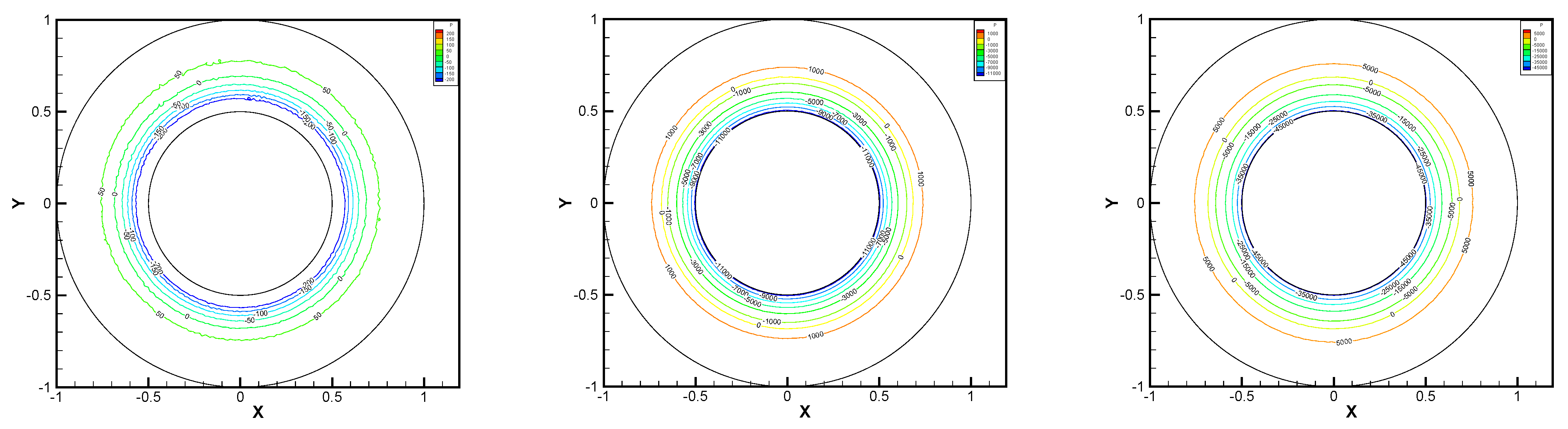
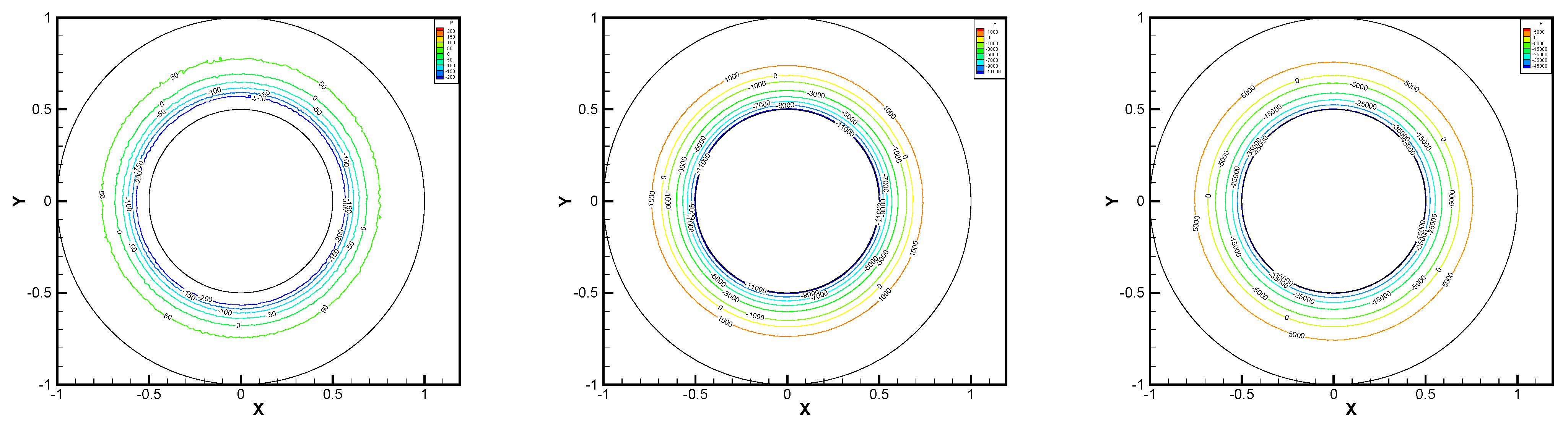
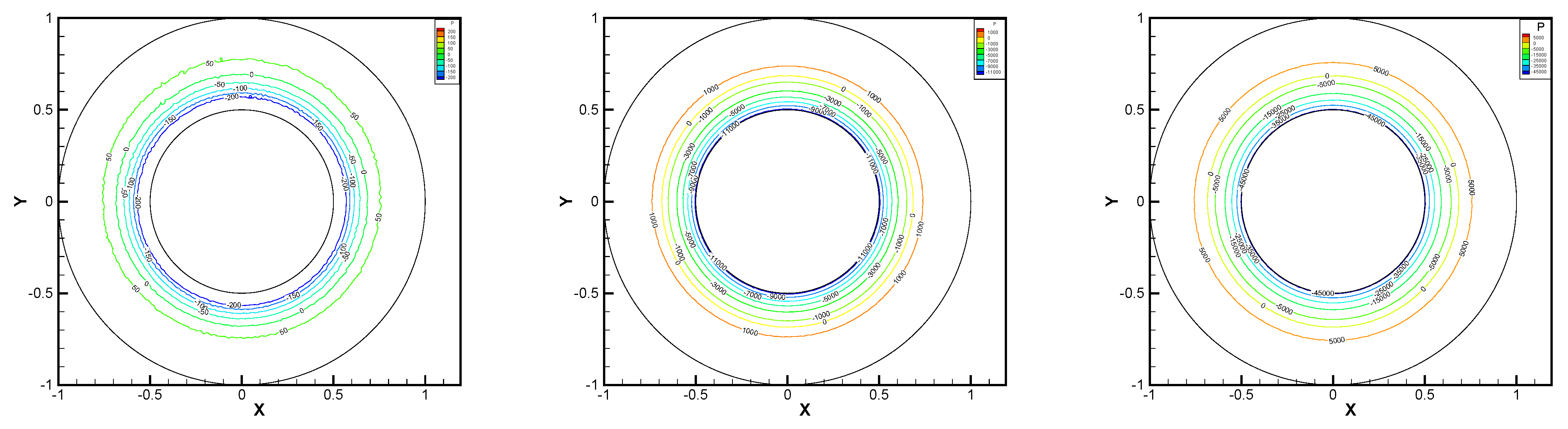
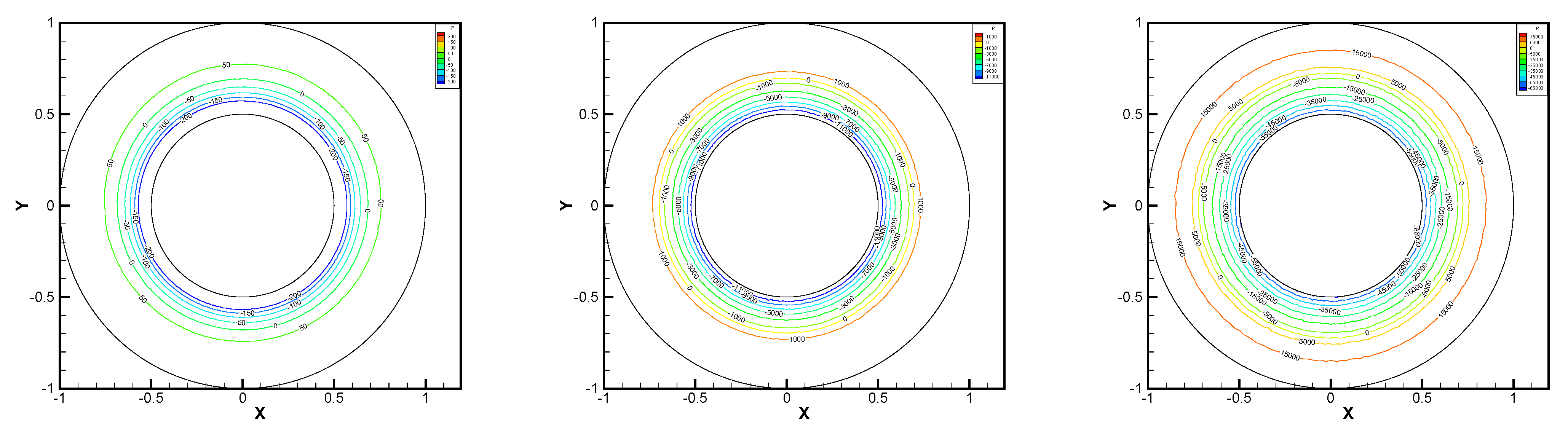
Figure 8.
, pressure level lines for the penalty method.
Figure 8.
, pressure level lines for the penalty method.
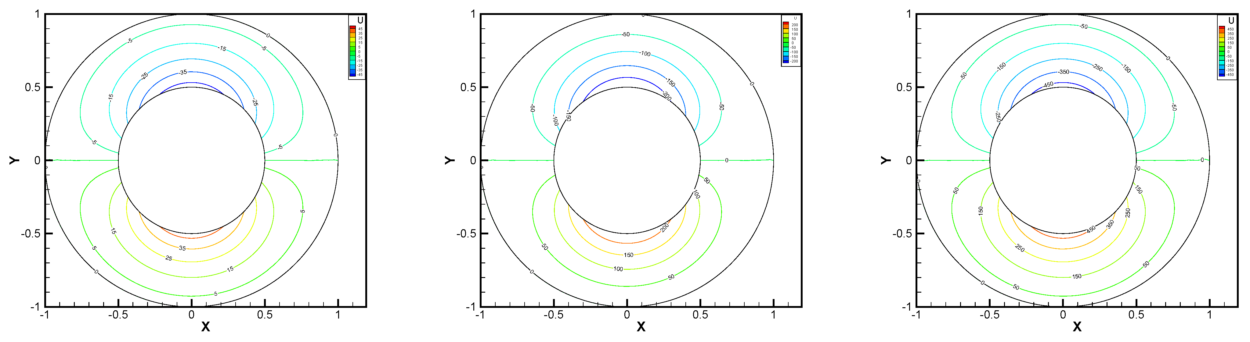
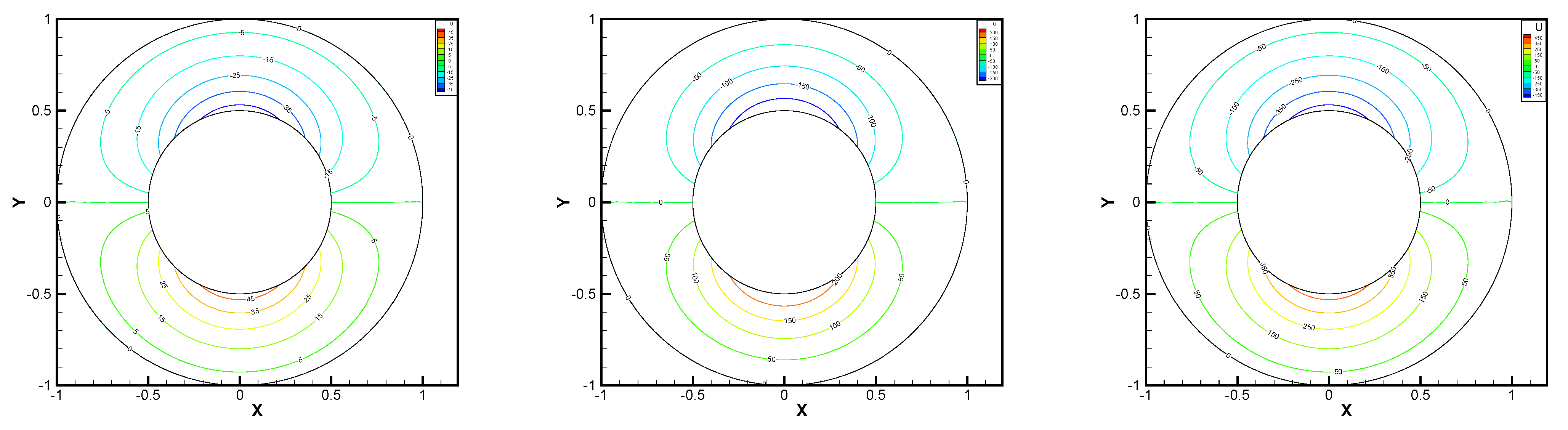
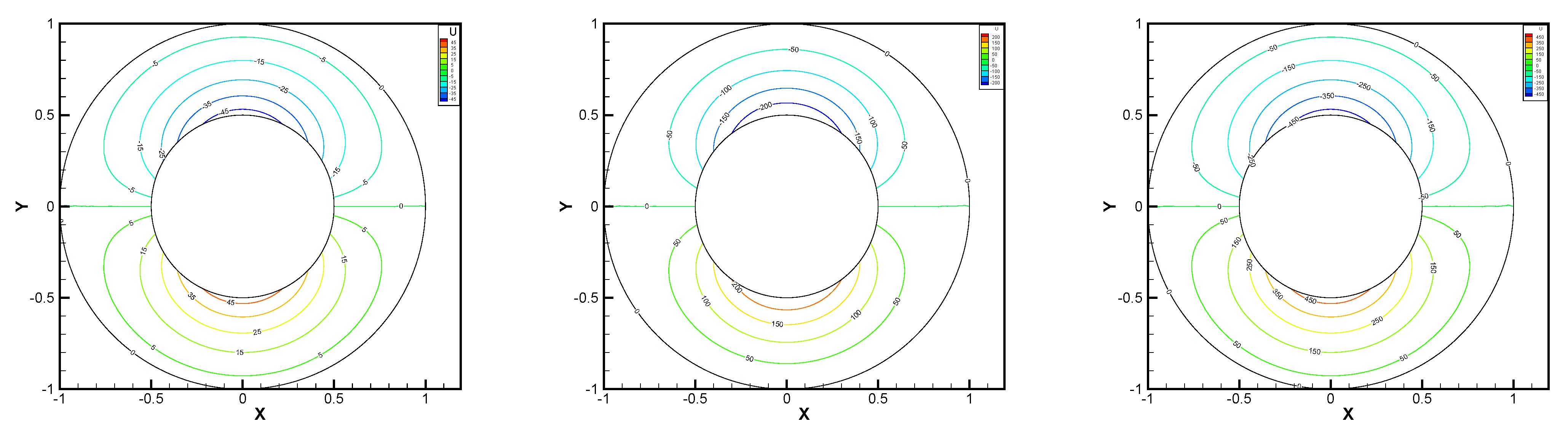
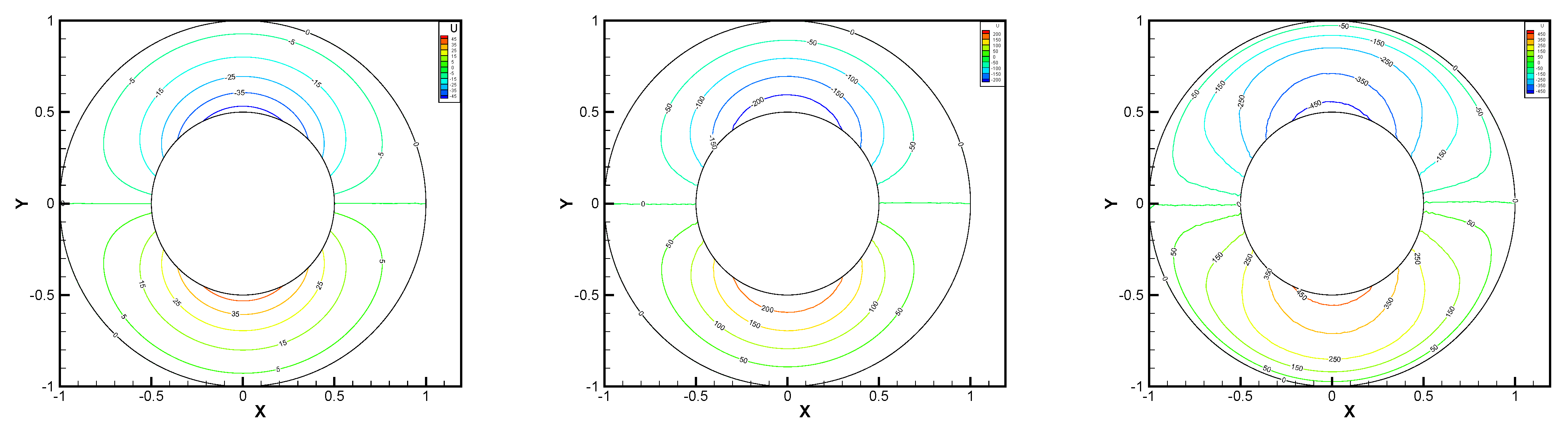
Figure 9.
, horizontal velocity for the penalty method.
Figure 9.
, horizontal velocity for the penalty method.
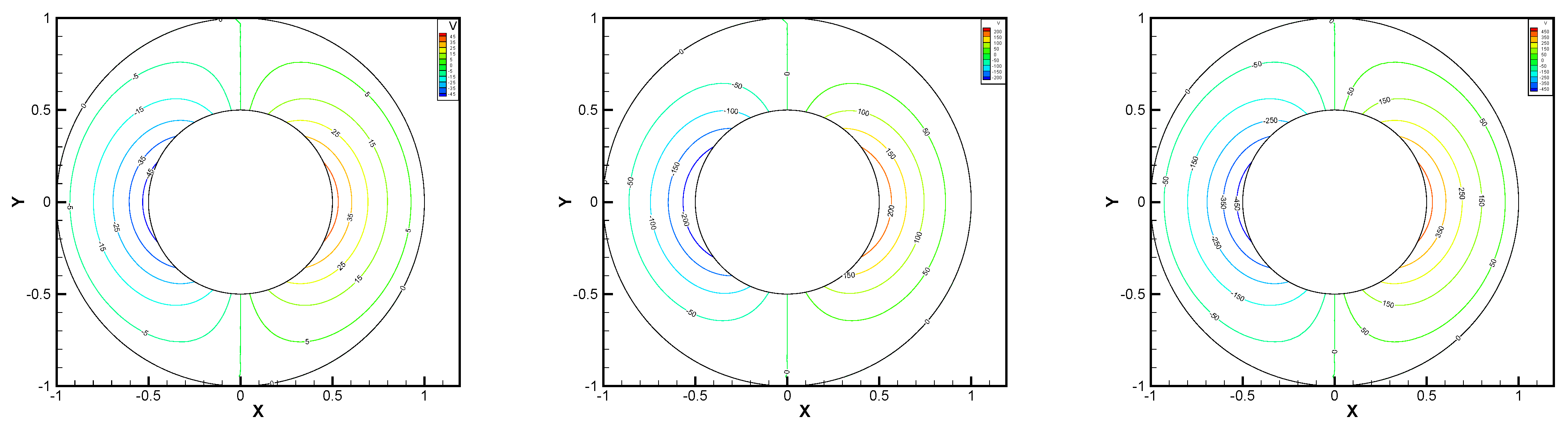
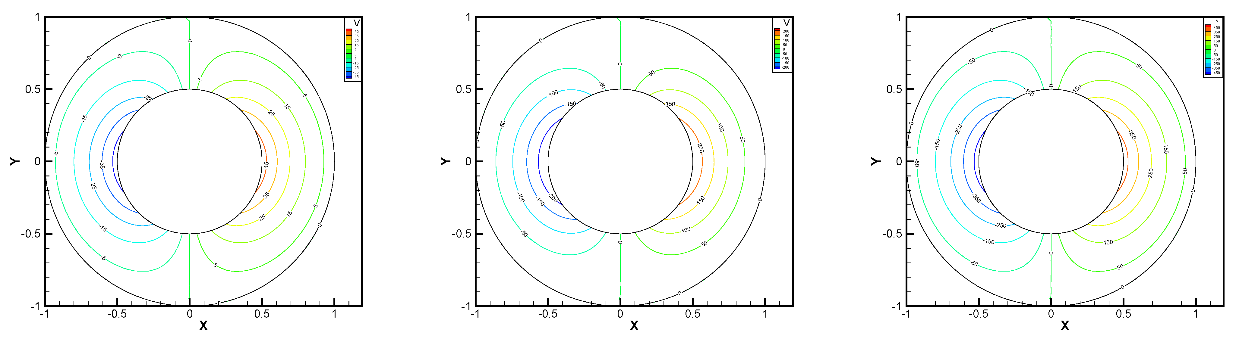
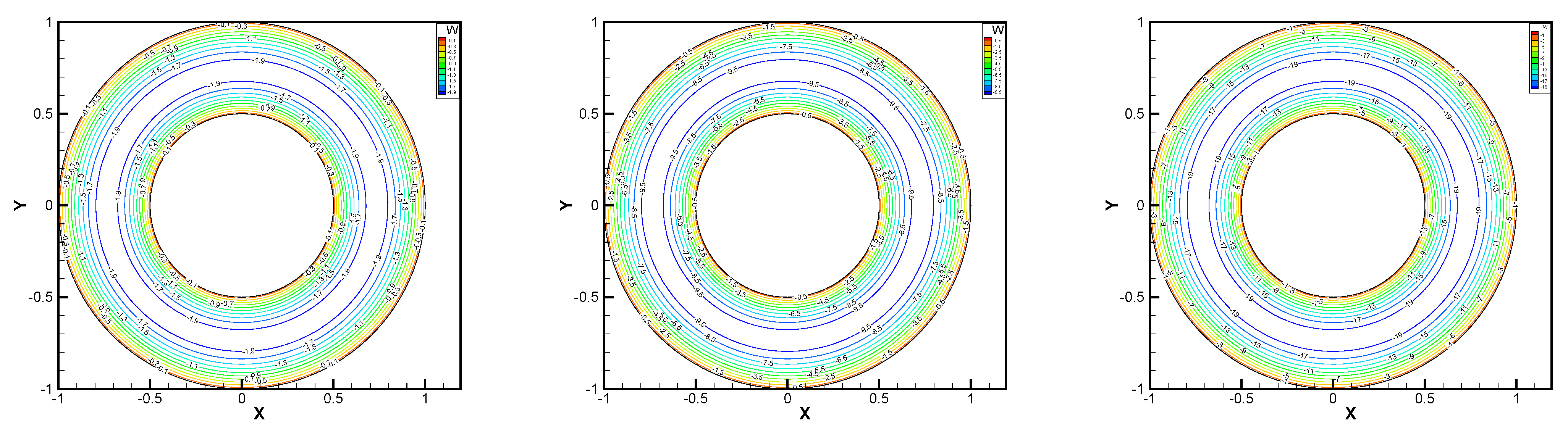
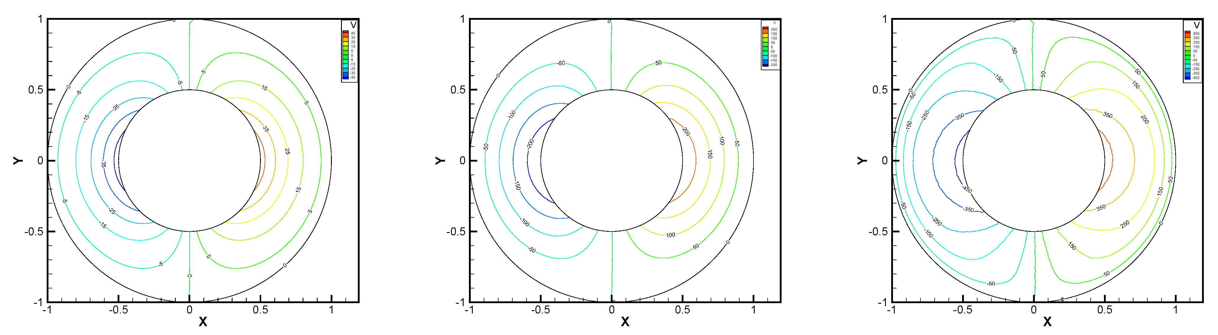
Figure 10.
, vertical velocity for the penalty method.
Figure 10.
, vertical velocity for the penalty method.
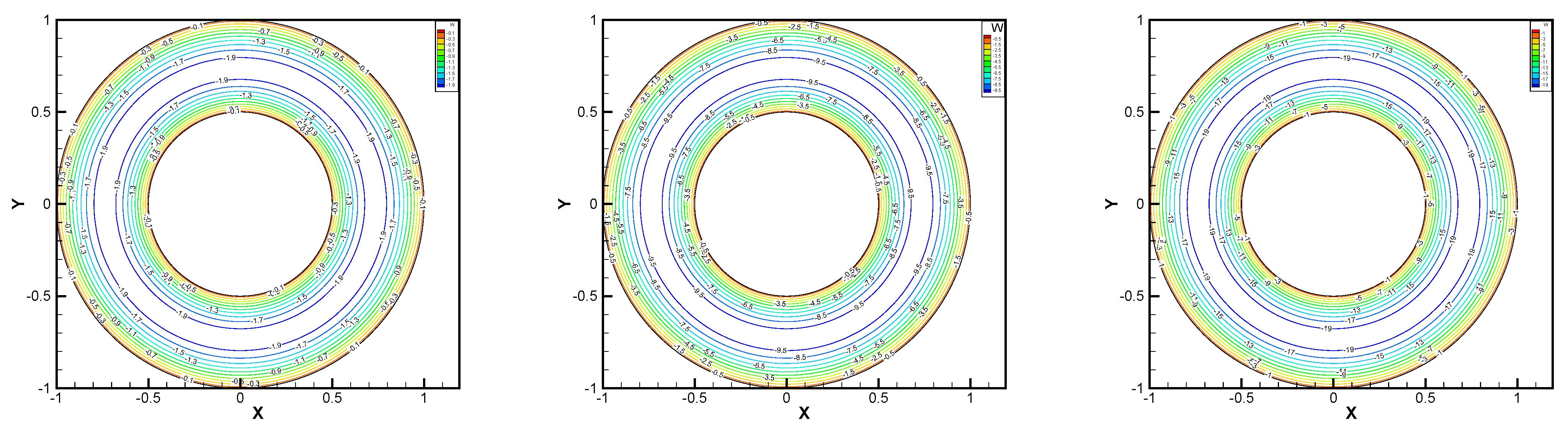
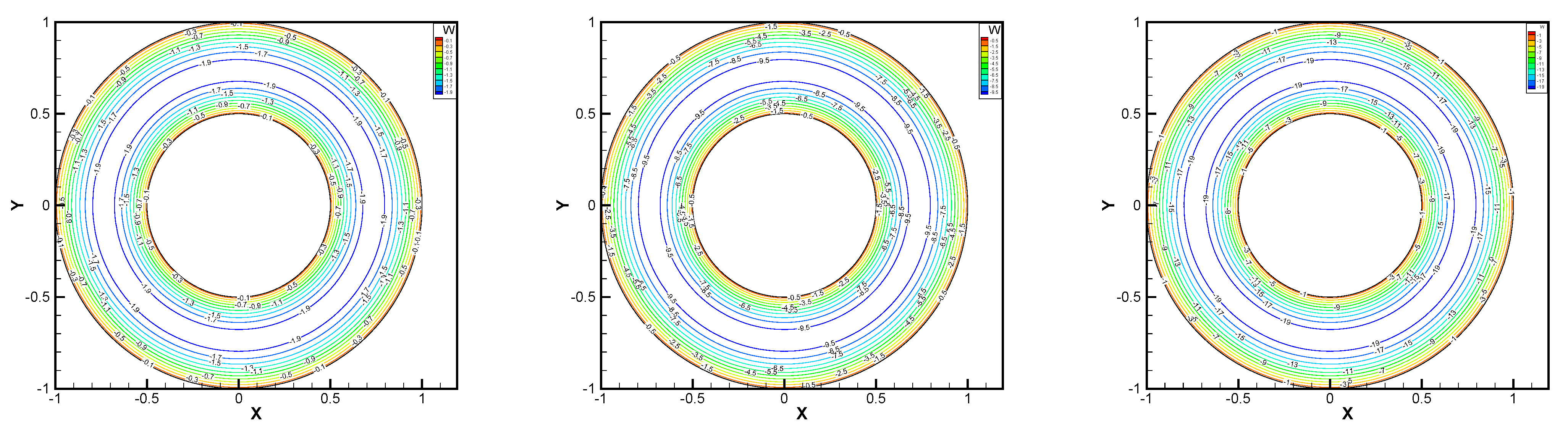
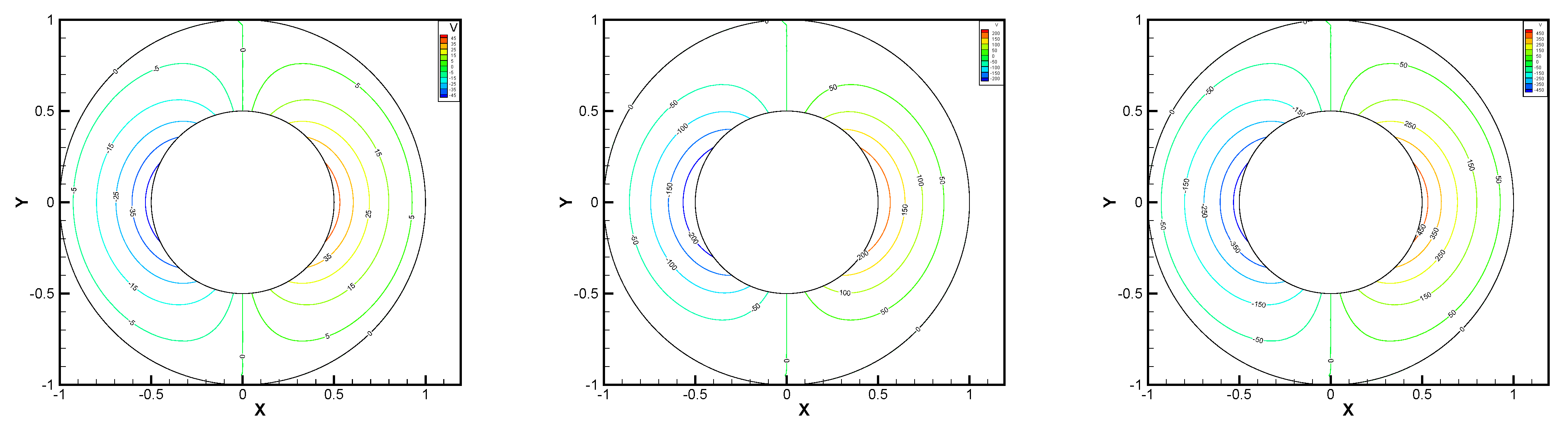
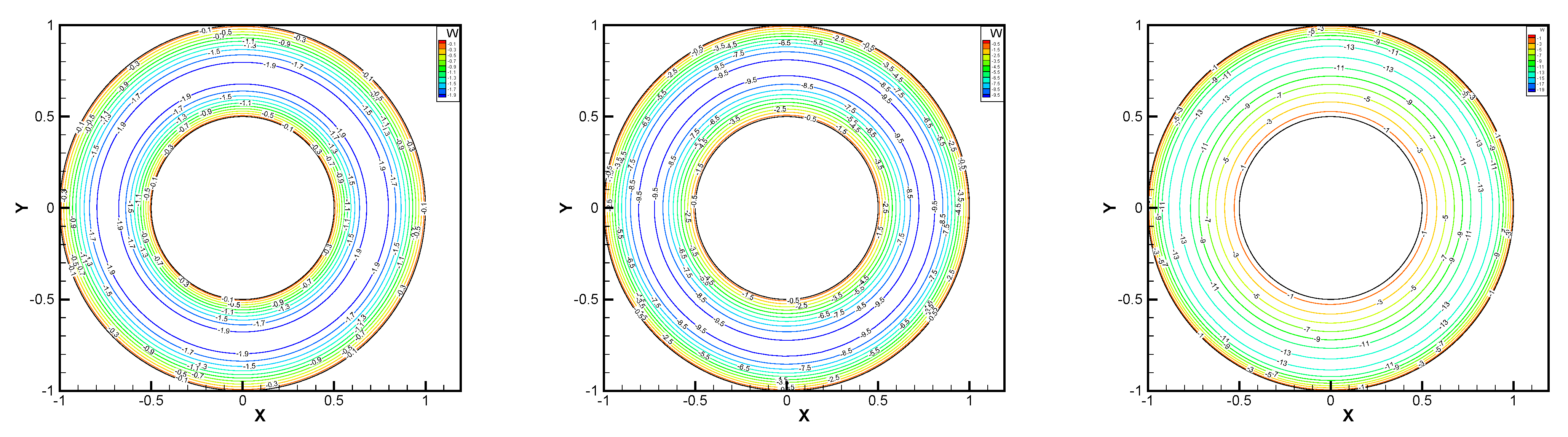
Figure 11.
, angular velocity for the penalty method.
Figure 11.
, angular velocity for the penalty method.
Figure 12.
, pressure level lines for the regular method.
Figure 12.
, pressure level lines for the regular method.
Figure 13.
, horizontal velocity for the regular method.
Figure 13.
, horizontal velocity for the regular method.
Figure 14.
, vertical velocity for the regular method.
Figure 14.
, vertical velocity for the regular method.
Figure 15.
, angular velocity for the regular method.
Figure 15.
, angular velocity for the regular method.
Figure 16.
, pressure level lines for the multiscale enrichment method.
Figure 16.
, pressure level lines for the multiscale enrichment method.
Figure 17.
, horizontal velocity for the multiscale enrichment method.
Figure 17.
, horizontal velocity for the multiscale enrichment method.
Figure 18.
, vertical velocity for the multiscale enrichment method.
Figure 18.
, vertical velocity for the multiscale enrichment method.
Figure 19.
, angular velocity for the multiscale enrichment method.
Figure 19.
, angular velocity for the multiscale enrichment method.
Figure 20.
, pressure level lines for the local Gauss integration method.
Figure 20.
, pressure level lines for the local Gauss integration method.
Figure 21.
, horizontal velocity for the local Gauss integration method.
Figure 21.
, horizontal velocity for the local Gauss integration method.
Figure 22.
, vertical velocity for the local Gauss integration method.
Figure 22.
, vertical velocity for the local Gauss integration method.
Figure 23.
, angular velocity for the local Gauss integration method.
Figure 23.
, angular velocity for the local Gauss integration method.
Table 1.
Typical structured mesh with for the penalty method.
Table 1.
Typical structured mesh with for the penalty method.
| CPU | | -Rate | | -Rate | | -Rate |
|---|
| 12 | 0.071 | | | | | | |
| 24 | 0.320 | 0.4089 | | 0.4948 | | 0.6529 | |
| 36 | 0.846 | 0.4332 | | 0.4873 | | 0.5985 | |
| 48 | 1.755 | 0.4440 | | 0.4841 | | 0.5683 | |
| 60 | 3.185 | 0.4505 | | 0.4826 | | 0.5497 | |
| 72 | 5.332 | 0.4551 | | 0.4819 | | 0.5373 | |
Table 2.
Typical structured mesh with for the penalty method.
Table 2.
Typical structured mesh with for the penalty method.
| CPU | | -Rate | | -Rate | | -Rate | | -Rate |
|---|
| 12 | 0.046 | | | | | | | | |
| 24 | 0.225 | | 2.018 | | 1.012 | | 1.991 | | 0.917 |
| 36 | 0.668 | | 2.014 | | 1.008 | | 1.999 | | 0.890 |
| 48 | 1.47 | | 2.010 | | 1.006 | | 2.000 | | 0.836 |
| 60 | 2.806 | | 2.008 | | 1.005 | | 2.001 | | 0.772 |
| 72 | 4.965 | | 2.005 | | 1.005 | | 2.001 | | 0.704 |
Table 3.
Typical structured mesh for the regular method.
Table 3.
Typical structured mesh for the regular method.
| CPU | | -Rate | | -Rate | | -Rate | | -Rate |
|---|
| 12 | 0.053 | | | | | | | | |
| 24 | 0.281 | | 2.012 | | 1.307 | | 1.990 | | 1.726 |
| 36 | 0.734 | | 2.016 | | 1.268 | | 1.998 | | 1.671 |
| 48 | 1.517 | | 2.013 | | 1.226 | | 1.999 | | 1.641 |
| 60 | 2.768 | | 2.011 | | 1.195 | | 2.000 | | 1.619 |
| 72 | 4.65 | | 2.010 | | 1.171 | | 2.000 | | 1.604 |
Table 4.
Typical structured mesh for the multiscale enrichment method.
Table 4.
Typical structured mesh for the multiscale enrichment method.
| CPU | | -Rate | | -Rate | | -Rate | | -Rate |
|---|
| 12 | 0.1 | | | | | | | | |
| 24 | 0.529 | | 1.960 | | 1.304 | | 1.940 | | 1.719 |
| 36 | 1.446 | | 1.936 | | 1.259 | | 1.919 | | 1.668 |
| 48 | 3.112 | | 1.900 | | 1.216 | | 1.888 | | 1.638 |
| 60 | 5.755 | | 1.863 | | 1.183 | | 1.853 | | 1.617 |
| 72 | 9.652 | | 1.825 | | 1.158 | | 1.817 | | 1.602 |
Table 5.
Typical structured mesh for the local Gauss integration method.
Table 5.
Typical structured mesh for the local Gauss integration method.
| CPU | | -Rate | | -Rate | | -Rate | | -Rate |
|---|
| 12 | 0.054 | | | | | | | | |
| 24 | 0.256 | | 2.012 | | 1.396 | | 1.991 | | 1.809 |
| 36 | 0.682 | | 2.009 | | 1.297 | | 1.999 | | 1.739 |
| 48 | 1.357 | | 2.006 | | 1.232 | | 2.000 | | 1.700 |
| 60 | 2.403 | | 2.003 | | 1.189 | | 2.001 | | 1.672 |
| 72 | 3.938 | | 2.000 | | 1.159 | | 2.001 | | 1.652 |
Table 6.
Unstructured mesh for the penalty method.
Table 6.
Unstructured mesh for the penalty method.
| | -Rate | | -Rate | | -Rate | | -Rate |
|---|
| 0.270282 | | | | | | | | |
| 0.14633 | | 2.91 | | 0.77 | | 2.39 | | 3.69 |
| 0.073319 | | 3.07 | | 1.95 | | 2.01 | | 1.98 |
| 0.0368164 | | 2.66 | | 1.61 | | 2.03 | | 1.77 |
| 0.0188245 | | 2.28 | | 1.20 | | 2.07 | | 2.06 |
Table 7.
Unstructured mesh for the regular method.
Table 7.
Unstructured mesh for the regular method.
| | -Rate | | -Rate | | -Rate | | -Rate |
|---|
| 0.270282 | | | | | | | | |
| 0.14633 | | 2.16 | | 1.14 | | 2.35 | | 1.81 |
| 0.073319 | | 2.01 | | 1.02 | | 2.01 | | 1.89 |
| 0.0368164 | | 2.02 | | 1.02 | | 2.03 | | 1.83 |
| 0.0188245 | | 2.05 | | 1.04 | | 2.08 | | 1.72 |
Table 8.
Unstructured mesh for the multiscale enrichment method.
Table 8.
Unstructured mesh for the multiscale enrichment method.
| | -Rate | | -Rate | | -Rate | | -Rate |
|---|
| 0.270282 | | | | | | | | |
| 0.14633 | | 1.89 | | 1.15 | | 2.11 | | 1.41 |
| 0.073319 | | 1.76 | | 1.03 | | 1.85 | | 1.74 |
| 0.0368164 | | 1.66 | | 1.01 | | 1.78 | | 1.61 |
| 0.0188245 | | 1.47 | | 1.01 | | 1.63 | | 1.42 |
Table 9.
Unstructured mesh for the local Gauss integration method.
Table 9.
Unstructured mesh for the local Gauss integration method.
| | -Rate | | -Rate | | -Rate | | -Rate |
|---|
| 0.270282 | | | | | | | | |
| 0.14633 | | 2.26 | | 1.12 | | 2.33 | | 1.37 |
| 0.073319 | | 2.03 | | 1.02 | | 2.01 | | 1.70 |
| 0.0368164 | | 2.04 | | 1.02 | | 2.03 | | 1.70 |
| 0.0188245 | | 2.07 | | 1.04 | | 2.07 | | 1.61 |


