Article

Numerical Study of Entropy Generation in Fully Developed Turbulent Circular Tube Flow Using an Elliptic Blending Turbulence Model

1
College of Civil and Transportation Engineering, Shenzhen University, Shenzhen 518060, China
2
Key Laboratory for Resilient Infrastructures of Coastal Cities (MOE), Shenzhen University, Shenzhen 518060, China
*
Author to whom correspondence should be addressed.
Entropy 2022, 24(2), 295; https://doi.org/10.3390/e24020295
Submission received: 7 January 2022 / Revised: 7 February 2022 / Accepted: 17 February 2022 / Published: 19 February 2022

Abstract

:
As computational fluid dynamics (CFD) advances, entropy generation minimization based on CFD becomes attractive for optimizing complex heat-transfer systems. This optimization depends on the accuracy of CFD results, such that accurate turbulence models, such as elliptic relaxation or elliptic blending turbulence models, become important. The performance of a previously developed elliptic blending turbulence model (the SST   k ω φ α model) to predict the rate of entropy generation in the fully developed turbulent circular tube flow with constant heat flux was studied to provide some guidelines for using this class of turbulence model to calculate entropy generation in complex systems. The flow and temperature fields were simulated by using a CFD package, and then the rate of entropy generation was calculated in post-processing. The analytical correlations and results of two popular turbulence models (the realizable kε and the shear stress transport (SST) kω models) were used as references to demonstrate the accuracy of the SST   k ω φ α model. The findings indicate that the turbulent Prandtl number (Prt) influences the entropy generation rate due to heat-transfer irreversibility. Prt = 0.85 produces the best results for the SST   k ω φ α model. For the realizable kε and SST kω models, Prt = 0.85 and Prt = 0.92 produce the best results, respectively. For the realizable kε and the SST kω models, the two methods used to predict the rate of entropy generation due to friction irreversibility produce the same results. However, for the SST   k ω φ α model, the rates of entropy generation due to friction irreversibility predicted by the two methods are different. The difference at a Reynolds number of 100,000 is about 14%. The method that incorporates the effective turbulent viscosity should be used to predict the rate of entropy generation due to friction irreversibility for the SST   k ω φ α model. Furthermore, when the temperature in the flow field changes dramatically, the temperature-dependent fluid properties must be considered.

1. Introduction

Due to the shortage of fossil energy and a desire for sustainable development, the demand for high-efficiency heat-transfer systems is increasing. Hence, much effort has been made to improve the efficiency of heat-transfer systems. However, much of this work is based on the first law of thermodynamics, which can provide a lot of useful information but does not provide optimal conditions. The entropy generation analysis (EGA), which is based on the second law of thermodynamics, is a powerful tool for heat-transfer-process optimization.
The EGA has been used in designing and optimizing thermal systems since its introduction by Bejan [1,2]. However, because earlier attempts were primarily theoretical, they could only deal with simple geometry configurations and flow conditions. Furthermore, some empirical correlations had to be introduced, because obtaining local information is difficult [3,4,5]. Flow and temperature fields can be obtained with the advancement of computational fluid dynamics (CFD), allowing the local entropy production to be computed. It is important for optimizing complex systems, because precise policy implementation is possible using local information. CFD has been used as a tool to evaluate the entropy generation and further optimize heat-transfer systems by a few researchers. Because the flow in many heat-transfer systems is turbulent, the turbulence characteristics must be considered. The Reynolds averaged Navier–Stokes (RANS)-based kε and kω models are the most commonly used turbulence models for calculating entropy generation. To avoid verbosity, only a few of them are discussed here. Shuja et al. [6] used four turbulence models to calculate the local entropy generation in a fluid jet impinging on a heated wall: the standard kε model, the low Reynolds number (Re) kε model, and two Reynolds stress models. Mwesigye et al. [7] used the realizable kε model to perform a numerical analysis of entropy generation in a parabolic trough receiver. Saqr et al. [8] investigated the entropy generation in a swirl pipe flow, using the realizable kε model. Wang et al. [9] modeled the flow around the NACA0012 airfoil and discussed the effect of turbulence models on entropy generation, using five turbulence models, namely the standard kε model, renormalization group (RNG) kε model, standard kω model, shear stress transport (SST) kω model, and Spalart–Allmaras (S–A) model. Ghorani et al. [10] used the entropy-generation-rate method with the SST kω model to investigate the flow within a centrifugal pump in a reverse mode. Yu et al. [11] investigated the detailed characteristics of the entropy production rate by simulating the flow in the Francis turbine, using the SST kω model. They also studied the effect of the mass flow rate on the entropy generation in the Francis turbine [12]. Pidaparthi et al. [13] analyzed and optimized the heat-transfer performance in a tube with internal helical fins by using EAG with the realizable kε model. Heat-transfer optimization of nanofluids by using EGA has also received attention. For example, Bianco et al. used the standard kε model to investigate the turbulent convection of Al2O3–water nanofluid inside a circular section tube subjected to constant heat flux [14] and constant wall temperature [15]. Mwesigye and Huan [16] investigated the turbulent nanofluid flow in a circular tube, using the entropy-generation-minimization method, with the help of a realizable kε model. Rashidi et al. [17] compared the single- and two-phase modeling approaches for heat-transfer performance in forced convection flow of TiO2-water nanofluid through EGA with the standard kε model. Bazdidi-Tehrani et al. [18] investigated the entropy generation in a CuO-water nanofluid flowing in a vertical duct, using the SST kω model. The SST kω model was also used by Fadodun et al. [19] to investigate the entropy production rate in a nanofluid flowing through an inwardly corrugated pipe in a turbulent flow regime. Bahiraei et al. [20] investigated the entropy generation in a nanofluid flow in a shell-and-tube heat exchanger with the RNG kε model.
Obviously, the accuracy of the flow and temperature fields predicted in CFD simulations affect the computing accuracy of local entropy generation. It is well-known that the kε and kω models have limitations when used in complex systems. Another type of RANS-based turbulence model, the elliptic relaxation model, or the elliptic blending model, which has been shown to outperform the kε and kω models in some complex systems, such as the 2D asymmetric diffuser flow, the sudden expansion pipe flow and the impinging jet flow [21,22], is expectedly more attractive for calculating local entropy generation. However, the application of such turbulence models in research on entropy generation has not been found in the literature, and this aspect has yet to be attempted.
This study investigated the performance of an elliptic-blending turbulence model developed in our previous work [22] to predict the local entropy generation rate in fully developed turbulent flows in a circular tube with constant heat flux. The purpose is to provide some guidelines for using this class of turbulence model to calculate entropy generation in complex systems. The accuracy of the elliptic-blending turbulence model was demonstrated by comparing it to the analytical correlations and the results of two other popular turbulence models (the realizable kε and the SST kω models). The computational method for entropy generation rate, the effect of the turbulent Prandtl number (Prt), the effect of large wall-fluid temperature difference, and the effect of the temperature-dependent fluid properties were investigated. The findings—for example, the Prt should be chosen as 0.85, the method that incorporates the effective turbulent viscosity should be used to predict the rate of entropy generation due to friction irreversibility, and the temperature-dependent fluid properties should be considered when the temperature difference is large—can guide the application of the elliptic blending turbulence model to complex problems.
The numerical modeling is briefly described in the next section. Then, in the third section, the results are presented and discussed in detail. Finally, the conclusions are presented.

2. Numerical Modeling

The problem under consideration is fully developed turbulent flow in a straight circular tube (diameter, D, and length, L) with a uniform constant heat flux ( q ) on the sidewall. Because of the axial symmetry of the problem under consideration, an axisymmetric computational model was constructed (Figure 1).

2.1. Governing Equations

The flow under consideration in this study is steady, incompressible, and turbulent. Turbulence was handled by using the Reynolds averaging method, yielding the steady RANS equations given as follows:
x i ( ρ u i ) = 0 ,
x j ( ρ u i u j ) = p x i + x j [ μ ( u i x j + u j x i ) ρ u i u j ¯ ]
For linear eddy viscosity turbulence models, the turbulent stresses are linked to the strain rate by using the following:
ρ u i u j ¯ = μ t ( u i x j + u j x i ) 2 3 ρ k δ i j
For incompressible flow, after using the Boussinesq approximation, the governing equation of energy can be simplified to the mean temperature (T) equation, as given by the following:
ρ T t + x i ( ρ u i T ) = x j [ ( μ Pr + μ t Pr t ) T x j ] .
The turbulence model yields the eddy viscosity, μt. The authors’ previously developed SST-incorporated elliptic-blending turbulence model (denoted as SST   k ω φ α model) was used. The model comprises four equations for the turbulent kinetic energy, k; specific dissipation rate, ω; wall-normal turbulent anisotropy, φ ; and elliptic variable, α, respectively. The following are the model equations.
ρ k t + x i ( ρ u i k ) = G k ρ f k β k ω + x j [ ( μ 2 + σ k μ t ) k x j ] ,
ρ ω t + x i ( ρ u i ω ) = f ω γ ω k G k ρ β ω 2 + C D + x j [ ( μ 2 + σ ω μ t ) ω x j ] ,
ρ φ t + x i ( ρ u i φ ) = ( 1 α p ) ρ f w a l l + α p ρ f hom φ k G k + 2 k μ t σ k φ x j k x j + x j [ ( μ 2 + σ φ μ t ) φ x j ] ,
0 = 1 α L 2 + x j ( α x j ) .
The eddy viscosity is defined by a blending formulation:
μ t = ( 1 α p ) C μ ρ φ k min ( T , T lim ) + α p a 1 ρ k max ( a 1 ω , F 2 S )
The model’s details are not provided here for the sake of brevity, and the interested reader is directed to Yang et al. [22]. Another two popular turbulence models, the realizable kε model [23] and the SST kω model [24], were also used for comparison.

2.2. Entropy Generations

In order to facilitate understanding, it is necessary to first declare the meaning of the superscripts on the rate of entropy generation, S, used in the following: ( · ) means the quantity per unit length, ( · ) means the quantity per unit area, and ( · ) means the quantity per unit volume.
The volumetric rate of entropy generation in viscous flow with convective heat transfer can be written as follows [3]:
S g e n = S g e n , f + S g e n , h ,
where the first and second terms on the right-hand side are the local volumetric rate of entropy generation due to friction irreversibility and heat transfer irreversibility, respectively. Both terms can be expressed in cylindrical coordinates for circular tube flow [3]:
S g e n , f = μ T { 2 [ ( u r r ) 2 + ( u r r ) 2 + ( u x x ) 2 ] + ( u x r + u r x ) 2 }
and
S g e n , h = λ T 2 [ ( T r ) 2 + ( T x ) 2 ] ,
where T is the local mean temperature of flow, and µ and λ are the molecular dynamic viscosity and the molecular thermal conductivity of the fluid, respectively. The volumetric rate of entropy generation is affected by absolute temperature, viscosity, thermal conductivity, and local spatial gradients of velocity and temperature. These quantities can be easily obtained by using CFD.
The two equations above are valid for laminar flow. For turbulent flow, there are two different processing methods when the mean values of the quantities are used to calculate the rate of entropy generation. One can still use Equations (11) and (12), but µ and λ must be replaced with effective viscosity (µ + µt) and effective thermal conductivity (λ + λt), respectively, where µt is the eddy viscosity and λt is the turbulent thermal conductivity [25,26]. Moreover, Equations (11) and (12) become the following:
S g e n , f = μ + μ t T { 2 [ ( u r r ) 2 + ( u r r ) 2 + ( u x x ) 2 ] + ( u x r + u r x ) 2 } ,
S g e n , h = λ + λ t T 2 [ ( T r ) 2 + ( T x ) 2 ] .
Another method was developed by Kock and Herwig [27]. Using the time-averaging process gives S g e n , f as follows:
S g e n , f = μ T { 2 [ ( u r r ) 2 + ( u r r ) 2 + ( u x x ) 2 ] + ( u x r + u r x ) 2 } + ρ ε T .
For S g e n , h , Equation (14) still holds. Equation (15) appears to have a natural advantage for kε models because the turbulence dissipation rate ε is obtained directly [28]. However, it could pose challenges to turbulence models where the accurate ε is difficult to obtain.
The following integral can be used to calculate the total rate of entropy generation in a fluid with volume, V:
S g e n = V S g e n d V = V ( S g e n , f + S g e n , h ) d V = S g e n , f + S g e n , h .
where
S g e n , f = V S g e n , f d V ,
S g e n , h = V S g e n , h d V .
For fully developed turbulent circular tube flow, Bejan [3] gave the analytical expressions for the rate of entropy generation per unit length as follows:
S g e n , f = 8 m ˙ 3 f π 2 ρ 2 T a v e 2 D 5 ,
S g e n , h = q 2 π λ T a v e 2 N u .
where Tave is the average temperature in the domain, f is the friction factor, m ˙   is the mass flow rate, q is the heat flux per unit length, and Nu is the Nusselt number.
For Nu, the widely used correlations are the Gnielinski’s correlation [29]:
N u = ( f / 8 ) ( Re 1000 ) Pr 1 + 12.7 ( f / 8 ) 0.5 ( Pr 2 / 3 1 ) ,
and the Dittus–Boelter correlation [29]:
N u = 0.023 Re 0.8 Pr 0.4 .
where Pr is the molecular Prandtl number. In Gnielinski’s correlation (Equation (21)), the friction factor is given by the Petukhov’s correlation [29]:
f = ( 0.79 ln Re 1.64 ) 2 .
This correlation can also be used in Equation (19) to calculate S g e n , f .

2.3. Numerical Procedures

The CFD package Ansys Fluent (17.0) was used for all computations. In addition, the User-Defined Function functionality was used to implement the SST   k ω φ α model. The four turbulence variables, k,   ω ,   φ , and α , were solved as User-Defined Scalar (UDS) quantities. The production and dissipation terms in these equations were added as “sources” to the transport equations, and the diffusivities of these variables were assigned accordingly. The SST kω and realizable kε models are pre-coded turbulence models available in Ansys Fluent that can be used directly.
The governing equations were solved by using the pressure-based Coupled algorithm. The second-order upwind scheme was used to discretize the convection terms in the momentum, energy, and turbulence equations. The velocity–pressure coupling process was handled by the Coupled algorithm, which solves the momentum and continuity equations in a closely coupled manner and can improve the rate of solution convergence significantly when compared to the segregated algorithm (such as the SIMPLE algorithm). The gradients and derivatives were evaluated by using the least-squares cell-based method. Furthermore, it should be noted that, in the current study, a double-precision solver was required to obtain a stable and accurate solution.
Figure 2 shows the solution procedures used in the present paper. For the cases considered in Section 3.1, Section 3.2, Section 3.3 and Section 3.4 (using the procedure as Figure 2a), the thermal properties of the materials were assumed to be temperature independent, allowing the governing equations for fluid flow and the energy equation to be solved independently. The isothermal fluid flow was solved first, and then the energy equation was solved by using the converged solution of the fluid flow. For the cases considered in Section 3.5 (using the procedure as Figure 2b), the temperature-dependent thermal properties of the fluid were considered, so that the governing equations for fluid flow and the energy equation were solved continuously in each iteration. After obtaining convergent flow and temperature fields, post-processing was performed to obtain the desired quantities, such as the Nusselt number, friction factor, and rate of entropy generation.

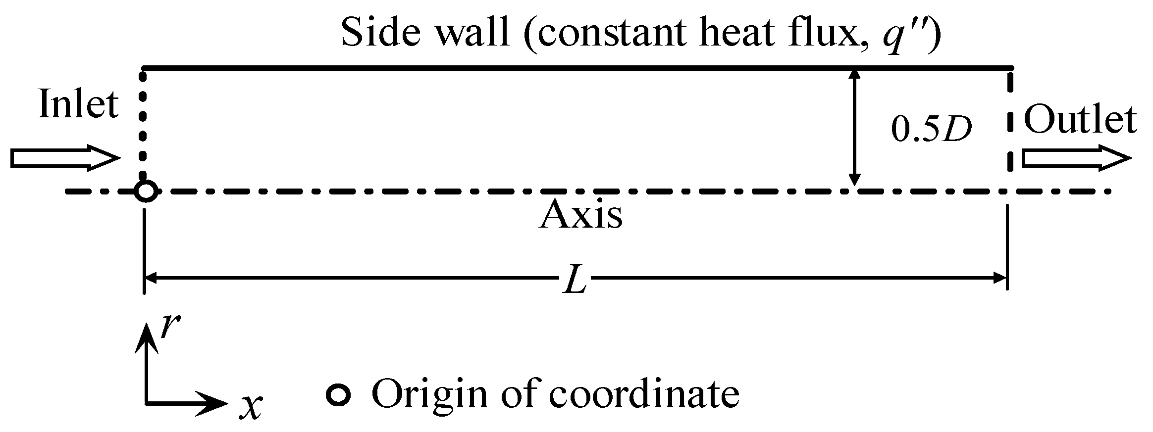
2.4. Computational Grid and Boundary Conditions

The computational domain (as shown in Figure 1) was meshed by using a Cartesian grid. In the vertical direction of the wall (r-direction), to capture high resolutions of variables close to the wall, the successive ratio mesh was used. In the streamwise direction (x-direction), the cells were distributed uniformly. Several different grids were designed to examine the mesh convergence results, and then we decided upon the grid used in the present work. In the test cases, the successive ratio and the number of nodes in the x-direction (Nx) kept being constants, as 1.05 and 100, respectively. The number of nodes in the r-direction (Nr) was different. Table 1 shows the results computed by using the SST   k ω φ α model with temperature-independent fluid properties. It was clear that, when Nr increases from 150 to 200, the change of the calculated parameters, f, Nu, S g e n , h ,   and   S g e n , f , whose reference values were evaluated by Equations (19)--(21), and (23), respectively, was small. Therefore, the mesh resolution of 200 × 100 was selected for the present work.
Figure 1 also depicts a schematic of the problem’s boundary conditions. Given that the turbulent flow in a circular tube is fully developed, it is appropriate to construct a periodic boundary condition for the inlet and outlet. The mass flow rate and temperature were specified at the inlet. To match the Re, the mass flow rate was adjusted. Throughout this study, the inlet temperature was 293.15 K. Constant heat flux was specified at the wall for the energy equation, and the no-slip condition was used for fluid flow. The wall treatments varied depending on the turbulence model. Specifically, for the SST   k ω φ α model, the conditions ui = 0, k = 0, φ = 0, α = 0, and ω = 3 ν / ( β 1 y 1 2 ) were specified [22]. For the SST kω model, an automatic near-wall treatment method was used [30]. The enhanced wall-treatment method was used for the realizable kε model [31].

2.5. Data Reduction

The results were obtained through post–processing. The Nusselt number, friction factor, and entropy generation rate per unit length were the relevant parameters used in the analysis. They were computed as follows.
The Nusselt number is denoted by the following:
N u ( x ) = h ( x ) D λ
where
h ( x ) = q T w ( x ) T m ( x ) ,
T m ( x ) = T i n + q π D x m ˙ c p
where h(x) is the local convective heat-transfer coefficient; q” is the heat flux; x is the distance from inlet; cp is the specific heat of the fluid; and Tin, Tw, and Tm are the inlet temperature, wall temperature, and bulk temperature, respectively. The average temperature Tave in Equations (19) and (20) is calculated as [14]
T a v e = T i n T m ( L ) ln ( T i n / T m ( L ) ) .
The friction factor is represented by the following:
f = 8 τ w ρ U b 2 .
where τ w is the wall shear stress, and Ub is the bulk velocity. Given that the aspect ratio of the computational region (L/D) is small in this work, the rates of entropy generation per unit length were calculated by using Equations (17) and (18) as follows:
S g e n , f = S g e n , f / L ,
S g e n , h = S g e n , h / L .

3. Results and Discussion

In present study, the working fluid is water, whose temperature-independent thermal properties at 293.15 K (used in Section 3.1, Section 3.2, Section 3.3 and Section 3.4) are listed in Table 2. For various purposes, three circular tubes with different cross-sectional areas (Ac) of 0.000005 m2, 0.0005 m2, and 0.05 m2; five Reynolds numbers, 10,000, 30,000, 50,000, 70,000, and 100,000; and different heat fluxes, ranging from 500 to 30,000 W/m2, were used. The main concern in this paper is the rate of entropy generation per unit length, which was obtained by averaging along the flow direction (Equations (29) and (30)). To achieve accurate results, it requires that the physical quantity in the computational region cannot change too much along the flow direction. Consequently, a value of 0.5 for the aspect ratio (L/D) was selected for all tubes considered in this study. Table 3 lists other parameters used in the following sections. For Section 3.1, Section 3.2 and Section 3.3, the motivation for using different heat fluxes for different tubes was to ensure that the wall-bulk temperature difference ( Δ T ) in all tubes was small enough when compared to the bulk flow temperature (Tm), and then the results could be compared with the analytical expressions of Bejan [3] (Equations (19) and (20)), in which the ratio of Δ T to Tm was small and, thus, ignored. However, we discovered that, when a large heat flux (for example, 50,000 W/m2) is applied to a large tube (for example, Ac = 0.05 m2), the computed rate of entropy generation deviates from the analytical expressions at a low Re. Mwesigye and Huan [16] discovered the same phenomenon. They reasoned that the large error was caused by the incorrect correlations used for Nu and f. However, we discovered in this study that Δ T is too large to be ignored in this case, and the condition that should be satisfied in Bejan’s analytical expression is violated.
The solution convergence history is influenced by the relaxation factors and the initial conditions. In present work, the relaxation factors for the four turbulent quantities of the SST   k ω φ α model were set to be 0.8, and the default values of the relaxation factors in the Ansys Fluent software were used for other quantities. The initial values (denoted by subscript 0) of the variables were set as follows: the turbulence intensity, I 0 = 0.03 ; the axial velocity, u 0 = μ Re ρ D ; the radial velocity, v 0 = 0 ,   k 0 = 1.5 ( u 0 I 0 ) 2 , ω 0 = k 0 0.5 0.0383 D , ε 0 = k 0 1.5 0.426 D , φ 0 = 0.3 ,   and   α 0 = 1.0 .
Based on same computer hardware (24 CPU cores with 3.1 GHz frequency and 128 GB RAM), the computational efficiency was compared by using a case with constant fluid properties and Ac = 0.05 m2, Re = 100,000, and q″ = 500 W/m2. The SST   k ω φ α , SST kω, and realizable kε models spent about 45, 32 and 28 min CPU time to obtain a convergent solution, respectively. The reason that the SST   k ω φ α model takes more computation time is that it has two more governing equations and more complex source terms.

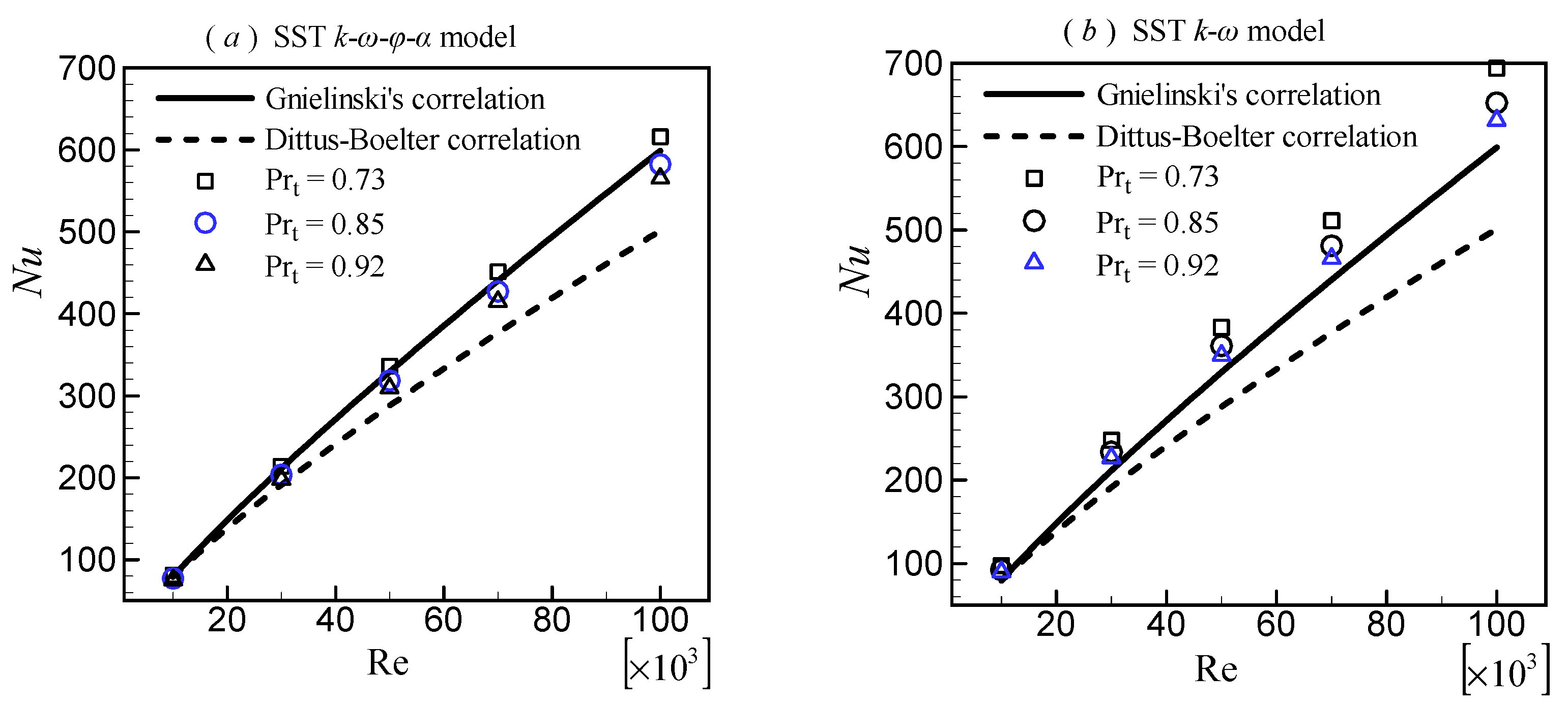
3.1. Validation of the Friction Factor and Nusselt Number

The friction factor was used to validate the hydrodynamic performance of the turbulence model. Figure 3 compares friction factors calculated by various turbulence models with Petukhov’s correlation [29]. The SST   k ω φ α model achieves an excellent agreement for all Re. The SST kω model and the realizable kε model both predict good results at high Re but overestimate the friction factor at low Re. When the Re is lower, the deviation is greater. This is not surprising given that both the SST kω model and the realizable kε model we used in present work are developed for high Re flow and do not include any low Re corrections, whereas the SST   k ω φ α model is developed for low and high Re flow and includes some low Re corrections.
The Nusselt number was used to validate the heat-transfer performance. It should be noted that the Prt in Equation (4) affects the temperature solution, which, in turn, affects other quantities, such as the Nusselt number, effective thermal conductivity, and rate of entropy generation. Because the influence factors are so complex and not fully understood, Prt is difficult to derive from theory. In CFD applications, Prt is typically treated by using an empirical formula or as a constant determined by the slope of the temperature curve in the log region [32]. Even in simple wall shear flows, there is no universal constant value for Prt. For example, the Prt ranges between 0.73 and 0.92 for airflow with Pr = 0.71 [32]. Furthermore, different turbulence models may necessitate different Prt, due to different temperature profile predictions. Three constant values, 0.73, 0.85, and 0.92, were used to evaluate the effect of Prt on heat-transfer performance.
The computed Nu by different Prt was compared with the Gnielinski’s correlation (Equation (21)) and the Dittus–Boelter correlation (Equation (22)). Figure 4 depicts the results. It is clear that a lower Prt leads to higher Nu for all turbulence models. All computed results deviate from the Dittus–Boelter correlation to a large extent. The results for the SST   k ω φ α model (Figure 4a) with Prt = 0.73 and 0.85 are in good agreement with Gnielinski’s correlation. The results with Prt = 0.92 deviate slightly. All results for the SST kω model (Figure 4b) deviate from Gnielinski’s correlation. The result with Prt = 0.92 is the best among them. The result with Prt = 0.85 for the realizable kε model (Figure 4c) is in good agreement with Gnielinski’s correlation. Prt = 0.73 overestimates the Nu. Prt = 0.92; however, underpredicts it.
Overall, the computed results for all three turbulence models agree better with the Gnielinski’s correlation than the Dittus–Boelter correlation, so the Gnielinski’s correlation was used where the correlation of Nu is required.

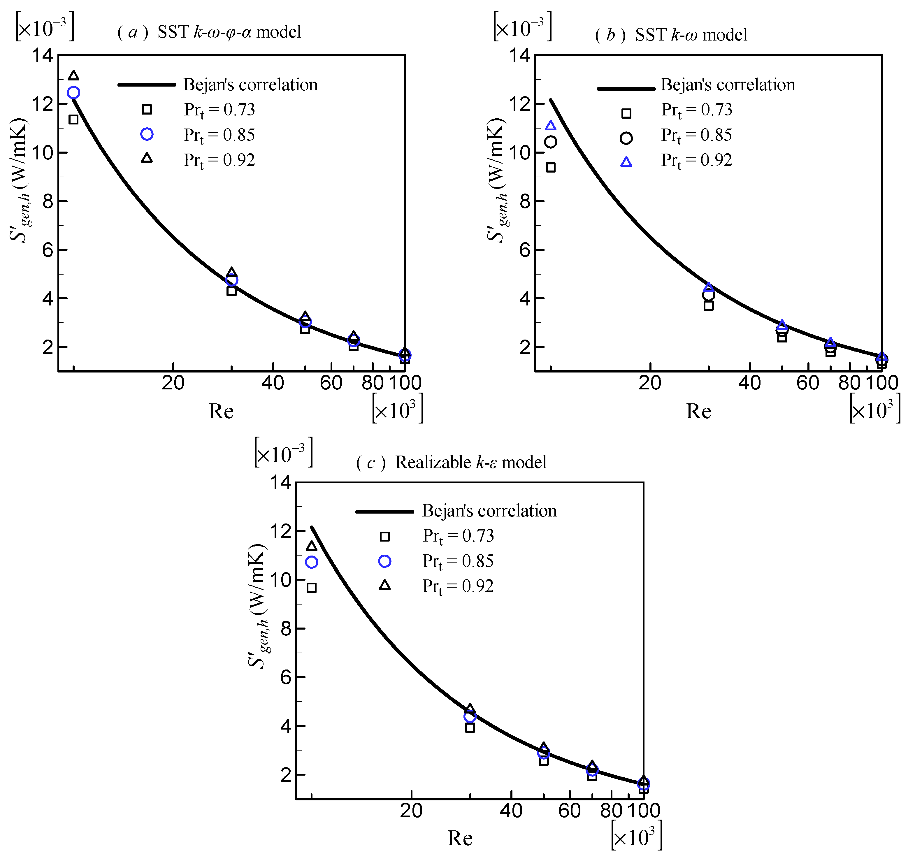
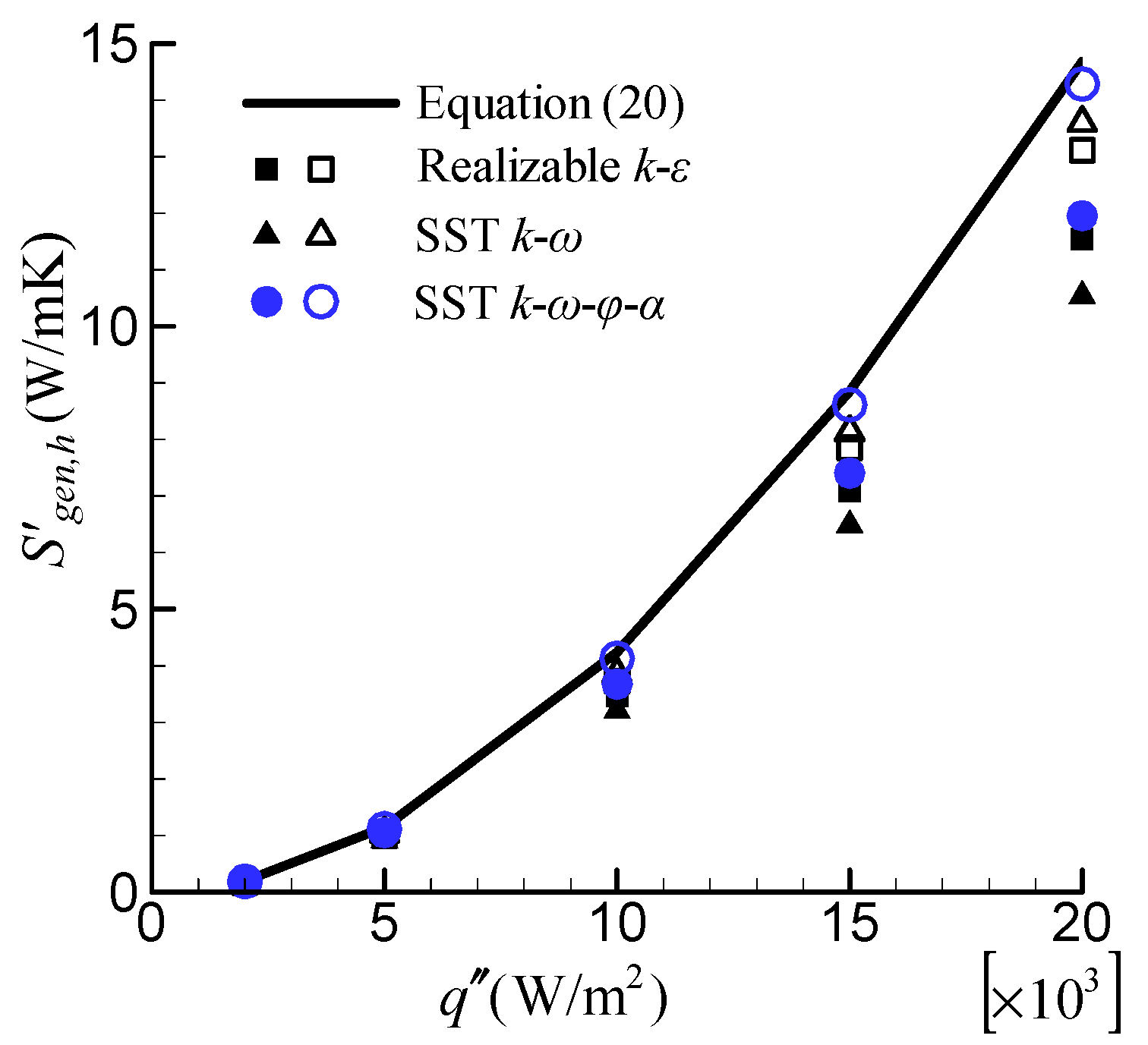
3.2. Rate of Entropy Generation Due to Heat Transfer Irreversibility

According to Equation (20), the rate of entropy generation per unit length due to heat transfer irreversibility, S g e n , h , is dependent on Tave and Nu, which is, in turn, dependent on Prt. Consequently, S g e n , h   will be affected by Prt. Because the effect of Prt on S g e n , h is similar for circular tubes of various sizes, only the results for Ac = 0.000005 m2 were provided. Figure 5 depicts the variation of S g e n , h with respect to Re computed by various turbulence models with varying Prt. It is self-evident that a smaller Prt results in a smaller   S g e n , h . This is the inverse of the effect of Prt on Nu. It is simple to understand because S g e n , h is inversely proportional to Nu. When comparing the SST   k ω φ α model (Figure 5a) with the Bejan’s correlation (Equation (20)), we see that the result with Prt = 0.85 agrees very well. Prt = 0.73 overpredicts but Prt = 0.92 underpredicts S g e n , h . Comparing the SST kω model (Figure 5b) with the Bejan’s correlation, we see that all values of Prt underpredict   S g e n , h , but the degree of deviation decreases as Re increases. The result with Prt = 0.92 is the best of the three Prt. The results with Prt = 0.85 for the realizable kε model (Figure 5c) agree with the Bejan’s correlation for high Re. However, for low Re (Re = 10,000), the result with Prt = 0.92 is better. Based on this finding, considering together the effect of Prt on Nu, the Prt that yields good Nu and S g e n , h was chosen in the subsequent analysis of each turbulence model, i.e., 0.85, 0.92, and 0.85 for the SST   k ω φ α model, SST kω model, and realizable kε model, respectively.
The local distribution of the rate of entropy generation per unit volume due to heat-transfer irreversibility, S g e n , h , along the radial direction at Re = 10,000 is shown in Figure 6. It can be seen that S g e n , h mainly occurs in the near-wall region. It is not surprising because, in the near-wall region, the temperature gradient is large. The distributions of S g e n , h predicted by the SST kω and realizable kε models are very close. The S g e n , h predicted by the SST   k ω φ α model is larger than the other two.

3.3. Rate of Entropy Generation Due to Friction Irreversibility

As mentioned in Section 2.2, there are two methods in CFD applications for calculating the entropy generation due to friction irreversibility,   S g e n , f . The first uses turbulent viscosity (Equation (13), denoted as Method 1), and the second uses the turbulent dissipation rate (Equation (15), denoted as Method 2). For the kε model series, Method 2 is natural. However, for other turbulence models in which ε is not easily determined, Method 2 may encounter difficulty. For example, in the SST   k ω φ α and SST kω models, although ε = β k ω was used when the models were developed, it does not hold everywhere due to some simplifications, modifications, and corrections.
Figure 7 depicts a comparison of the results obtained by using Methods 1 and 2. Because the observed phenomena are the same for tubes of different diameters, only the results with Ac = 0.000005 m2 are provided. The results show that S g e n , f increases with the increasing Re. For the SST   k ω φ α model, the results predicted by the two methods are significantly different. Compared with the Bejan’s correlation (Equation (19)), the result predicted by Method 1 agrees well, but the result predicted by Method 2 deviates. The difference at Re = 100,000 is about 14%. This is because the equation ε = β k ω does not exactly hold in the SST   k ω φ α model. Consequently, Method 2 cannot be used to determine S g e n , f for this model. However, for the SST kω and realizable kε models, the results predicted by the two methods are almost indistinguishable, and they are both in good agreement with the Bejan’s correlation.
Figure 8 shows the local distribution of the rate of entropy generation per unit volume due to friction irreversibility, S g e n , f , along the radial direction at Re = 10,000. Similar to S g e n , h , the S g e n , f mainly occurs in the near-wall region. This is because the velocity gradient is large in the near-wall region. The difference among three models occurs in a very thin region near the wall (0.49 < r/D < 0.5), so that, after being integrated, the difference is small.
As we can see from Equation (19), when the difference in average temperature is small, the S g e n , f is inversely proportional to the square of tube diameter at the same Re. This phenomenon is well represented by all three turbulence models. The details are omitted here for brevity.

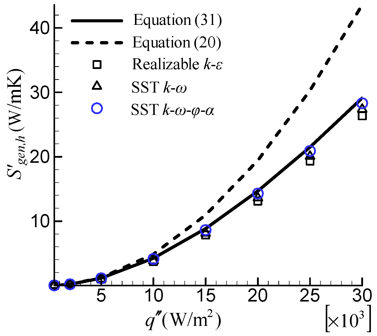
3.4. Rate of Entropy Generation Due to Heat Transfer Irreversibility with Large Δ T

As previously stated, Bejan’s correlation of the rate of entropy generation per unit length due to heat transfer irreversibility ( S g e n , h , Equation (20)) holds only if Δ T /Tm is so small that it can be ignored. In fact, when Δ T /Tm cannot be ignored, S g e n , h should be calculated by using the following [3].
S g e n , h = q Δ T T a v e ( T a v e + Δ T ) .
Considering Δ T = T w T m and q = π D q , using Equations (24) and (25) can yield
Δ T = q π λ N u .
The Bejan’s correlation will deviate significantly in the large tube with a high heat flux and low Re [16]. To investigate the turbulence model’s ability to predict S g e n , h when the wall-bulk temperature difference is large, the flow in a large tube with Ac = 0.05 m2 and a low Re of 10,000 was considered. Figure 9 compares the predicted S g e n , h by different turbulence models with the analytical results. In this case,   S g e n , h increases with increasing heat flux. All three turbulence models’ results agree well with the analytical expression of Equation (31). Among them, the SST   k ω φ α model predicts a better result. However, the deviation of the Bejan’s correlation (Equation (20)) is very noticeable and increases with increasing heat flux. The deviation is close to 50% at q = 30 , 000 W/m2. When examining this case in detail, we discovered that the large wall-bulk temperature difference (exceeding 100 K) is the reason for the large error. This finding suggests that, when using the Bejan’s correlation (Equation (20)) to validate turbulence models, it is critical to ensure that the wall-bulk temperature difference is small enough that Δ T /Tm can be ignored.

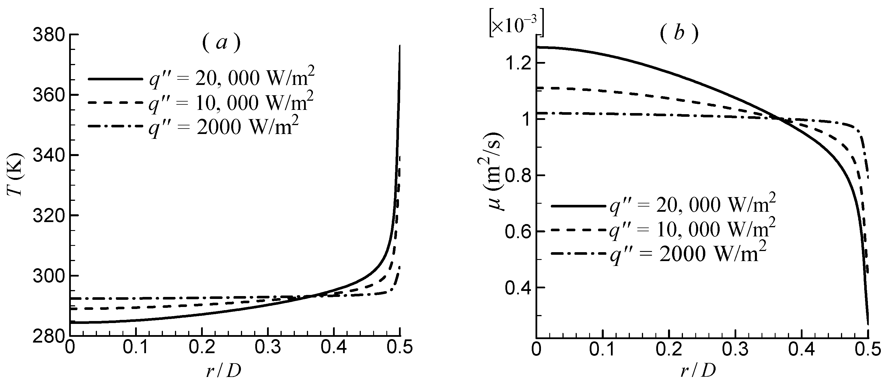
3.5. Effect of the Temperature-Dependent Fluid Properties

It is well-known that the properties of a fluid are generally temperature-dependent. For example, the viscosity of water is highly temperature-dependent. When the temperature changes significantly, it is inappropriate to consider fluid properties as constants. Ideally, the entropy generation rate will change because of temperature-dependent fluid properties on the flow field. Hence, the effect of temperature-dependent fluid properties on the entropy generation rate was investigated in this subsection. Abbasian Arani and Amani [33] used the following correlations to calculate the water properties.
ρ = 764.475639 + 19.25155 × T 0.07714568 × T 2 + 1.364893 × 10 4 × T 3 9.339158 × 10 8 × T 4 .
ln ( μ 0.001792 ) = 1.24 6.44 × ( 273.15 T ) + 7.68 × ( 273.15 T ) 2 .
c p = 198,531.690492 2894.853934 × T + 17.2363068 × T 2 0.05126994 × T 3 + 7.616133 × 10 5 × T 4 4.517821 × 10 8 × T 5 .
λ = 1.549404 + 0.01553952 × T 3.65967 × 10 5 × T 2 + 2.9401 × 10 8 × T 3 .
The flow in the tube with Ac = 0.05 m2 at Re = 10,000, which is based on fluid properties at the inlet (Tin = 293.15 K), was computed. Five cases were considered, each with a different heat flux of 2000, 5000, 10,000, 15,000, and 20,000 W/m2. Figure 10 depicts the effect of temperature-dependent fluid properties on entropy generation rate due to friction irreversibility, S g e n , f . The Bejan’s correlation of Equation (19) computed by using constant fluid properties at inlet temperature was included as a reference. The result of Bejan’s correlation decreases only slightly as heat flux increases. Conversely, as the heat flux increases, all S g e n , f computed by using CFD results with three turbulence models decreased significantly. The observed behavior can be explained by using detailed flow and temperature field information. Figure 11 depicts the SST   k ω φ α model’s simulated temperature and fluid molecular viscosity profiles on the lateral section. The difference in average temperature for different heat fluxes is small. Consequently, the S g e n , f predicted by the Bejan’s correlation with constant fluid property, which is only dependent on the average temperature, decreases slightly with increasing heat flux. With increasing heat flux in the near-wall region, the local temperature rises dramatically, significantly lowering the molecular fluid viscosity. Furthermore, there is a high velocity gradient near the wall. Consequently, the S g e n , f computed using CFD results (Equation (11)) are significantly reduced. The greater the heat flux, the lower the viscosity and, consequently, the entropy generation.
The effect of temperature-dependent fluid properties on the rate of entropy generation due to heat-transfer irreversibility, S g e n , h , is depicted in Figure 12. The CFD predicted S g e n , h separately, using temperature-dependent fluid properties (denoted by solid points), and constant fluid properties at inlet temperature (denoted by hollow points) were compared with the Bejan’s correlation of Equation (20). When considering the variation of fluid properties with temperature, S g e n , h is significantly reduced. Similar to S g e n , f , the greater the heat flux applied, the more S g e n , h decreases.
This result demonstrates that temperature-dependent fluid properties must be considered when there is a significant temperature change in the flow field. In this case, Bajen’s correlations are inapplicable.

4. Conclusions

The rate of entropy generation in a circular tube subjected to uniform heat flux was calculated by using an elliptic blending model ( SST   k ω φ α ). The analytical correlations and results that were computed by using the realizable kε model and the SST kω model were provided as references. As a result of the findings, the following conclusions were reached.
(1) The turbulent Prandtl number influences both the Nusselt number and the entropy generation rate due to heat-transfer irreversibility. For the SST   k ω φ α model, Prt = 0.85 yields the best results. The SST   k ω φ α model produces excellent results for all Reynolds numbers; however, both the realizable kε and SST kω models perform poorly for low Reynolds numbers.
(2) The rate of entropy generation due to friction irreversibility was well predicted by all three turbulence models. For the realizable kε and SST kω models, the two methods for calculating S g e n , f   led to nearly indistinguishable results. However, For the SST   k ω φ α model, the difference between two methods is significant and it is about 14% at Re = 100,000. The method that employs the effective turbulent viscosity, rather than the turbulent dissipation rate, ε, should be used.
(3) When the temperature in the flow field varies significantly, the change in fluid properties with a temperature considerably affects entropy generation rates due to friction and heat transfer.
In conclusion, the SST   k ω φ α model outperforms the other two turbulence models. Furthermore, although the case studied in this paper is relatively simple, given the inherent advantages of the SST   k ω φ α model in complex flows, it has great potential for the application of heat-transfer-system optimization. The application of this model in complex heat-transfer systems (such as separated flow and impinging jet flow) requires continued research and verification.
Finally, it should be pointed out that this paper mainly studied the capabilities of the turbulence model, rather than the detailed behavior of entropy generation rate in circular pipe flow, so we did not focus on the contribution of each part of the entropy generation rate to the total entropy generation rate. In fact, it could be clearly seen that, in small-sized pipe (Ac = 0.000005 m2), as shown in Section 3.3 and Section 3.4, the entropy generation rate due to heat transfer is only on the order of 10−3 of the entropy generation rate due to friction. Meanwhile, in large-sized pipe (Ac = 0.05 m2), as shown in Section 3.5, the entropy generation rate due to friction is only on the order of 10−7 of the entropy generation rate due to heat transfer. For the total entropy generation rate, the entropy generation rate due to heat transfer in small-sized pipe and that due to friction in large-sized pipe are completely negligible. Of course, for medium-sized pipes, the entropy generation rates of these two parts are of the same order of magnitude.

Author Contributions

Conceptualization, X.Y. and L.Y.; methodology, X.Y. and L.Y.; software, X.Y.; validation, L.Y.; writing—original draft preparation, X.Y.; writing—review and editing, L.Y. All authors have read and agreed to the published version of the manuscript.

Funding

This research was funded by the National Key R&D Program of China (Grant No. 2018YFB2100901) and the Natural Science Foundation of Shenzhen, China (Grant No. 20200814105851001).

Institutional Review Board Statement

Not applicable.

Informed Consent Statement

Not applicable.

Data Availability Statement

Not applicable.

Conflicts of Interest

The authors declare no conflict of interest.

References

  1. Bejan, A. A study of entropy generation in fundamental convective heat transfer. J. Heat Transf. 1979, 101, 718–725. [Google Scholar] [CrossRef]
  2. Sciacovelli, A.; Verda, V.; Sciubba, E. Entropy generation analysis as a design tool—A review. Renew. Sustain. Energy Rev. 2015, 43, 1167–1181. [Google Scholar] [CrossRef]
  3. Bejan, A. Entropy Generation Minimization: The Method of Thermodynamic Optimization on Finite-Size Systems and Finite-Time Processes; CRC Press: New York, NY, USA, 1996. [Google Scholar]
  4. Zimparov, V. Extended performance evaluation criteria for enhanced heat transfer surfaces: Heat transfer through ducts with constant wall temperature. Int. J. Heat Mass Transf. 2000, 43, 3137–3155. [Google Scholar] [CrossRef]
  5. Ratts, E.B.; Raut, A.G. Entropy generation minimization of fully developed internal flow with constant heat flux. J. Heat Transf. 2004, 126, 656–659. [Google Scholar] [CrossRef]
  6. Shuja, S.Z.; Yilbas, B.S.; Budair, M.O. Local entropy generation in an impinging jet: Minimum entropy concept evaluating various turbulence models. Comput. Methods Appl. Mech. Eng. 2001, 190, 3623–3644. [Google Scholar] [CrossRef]
  7. Mwesigye, A.; Bello-Ochende, T.; Meyer, J.P. Numerical investigation of entropy generation in a parabolic trough receiver at different concentration ratios. Energy 2013, 53, 114–127. [Google Scholar] [CrossRef] [Green Version]
  8. Saqr, K.M.; Shehata, A.I.; Taha, A.A.; Abo ElAzm, M.M. CFD modelling of entropy generation in turbulent pipe flow: Effects of temperature difference and swirl intensity. Appl. Therm. Eng. 2016, 100, 999–1006. [Google Scholar] [CrossRef]
  9. Wang, W.; Wang, J.; Liu, H.; Jiang, B.-y. CFD prediction of airfoil drag in viscous flow using the entropy generation method. Math. Probl. Eng. 2018, 2018, 4347650. [Google Scholar] [CrossRef] [Green Version]
  10. Ghorani, M.M.; Sotoude Haghighi, M.H.; Maleki, A.; Riasi, A. A numerical study on mechanisms of energy dissipation in a pump as turbine (PAT) using entropy generation theory. Renew. Energy 2020, 162, 1036–1053. [Google Scholar] [CrossRef]
  11. Yu, A.; Tang, Q.; Chen, H.; Zhou, D. Investigations of the thermodynamic entropy evaluation in a hydraulic turbine under various operating conditions. Renew. Energy 2021, 180, 1026–1043. [Google Scholar] [CrossRef]
  12. Yu, A.; Tang, Y.; Tang, Q.; Cai, J.; Zhao, L.; Ge, X. Energy analysis of Francis turbine for various mass flow rate conditions based on entropy production theory. Renew. Energy 2022, 183, 447–458. [Google Scholar] [CrossRef]
  13. Pidaparthi, B.; Li, P.; Missoum, S. Entropy-based optimization for heat transfer enhancement in tubes with helical fins. J. Heat Transf. 2022, 144, 012001. [Google Scholar] [CrossRef]
  14. Bianco, V.; Manca, O.; Nardini, S. Entropy generation analysis of turbulent convection flow of Al2O3–water nanofluid in a circular tube subjected to constant wall heat flux. Energy Convers. Manag. 2014, 77, 306–314. [Google Scholar] [CrossRef]
  15. Bianco, V.; Manca, O.; Nardini, S. Performance analysis of turbulent convection heat transfer of Al2O3 water-nanofluid in circular tubes at constant wall temperature. Energy 2014, 77, 403–413. [Google Scholar] [CrossRef]
  16. Mwesigye, A.; Huan, Z. Thermodynamic analysis and optimization of fully developed turbulent forced convection in a circular tube with water–Al2O3 nanofluid. Int. J. Heat Mass Transf. 2015, 89, 694–706. [Google Scholar] [CrossRef]
  17. Rashidi, M.M.; Nasiri, M.; Shadloo, M.S.; Yang, Z. Entropy generation in a circular tube heat exchanger using nanofluids: Effects of different modeling approaches. Heat Transf. Eng. 2017, 38, 853–866. [Google Scholar] [CrossRef]
  18. Bazdidi-Tehrani, F.; Vasefi, S.I.; Anvari, A.M. Analysis of particle dispersion and entropy generation in turbulent mixed convection of CuO-Water nanofluid. Heat Transf. Eng. 2019, 40, 81–94. [Google Scholar] [CrossRef]
  19. Fadodun, O.G.; Amosun, A.A.; Okoli, N.L.; Olaloye, D.O.; Ogundeji, J.A.; Durodola, S.S. Numerical investigation of entropy production in SWCNT/H2O nanofluid flowing through inwardly corrugated tube in turbulent flow regime. J. Therm. Anal. Calorim. 2020, 144, 1451–1466. [Google Scholar] [CrossRef]
  20. Bahiraei, M.; Naseri, M.; Monavari, A. A second law analysis on flow of a nanofluid in a shell-and-tube heat exchanger equipped with new unilateral ladder type helical baffles. Powder Technol. 2021, 394, 234–249. [Google Scholar] [CrossRef]
  21. Yang, X.L.; Yang, L.; Huang, Z.W.; Liu, Y. Development of a kωϕα turbulence model based on elliptic blending and applications for near-wall and separated flows. J. Turbul. 2017, 18, 36–60. [Google Scholar] [CrossRef]
  22. Yang, X.L.; Liu, Y.; Yang, L. A shear stress transport incorporated elliptic blending turbulence model applied to near-wall, separated and impinging jet flows and heat transfer. Comput. Math. Appl. 2020, 79, 3257–3271. [Google Scholar] [CrossRef]
  23. Shih, T.-H.; Liou, W.W.; Shabbir, A.; Yang, Z.; Zhu, J. A new k-ε eddy viscosity model for high Reynolds number turbulent flows. Comput. Fluids 1995, 24, 227–238. [Google Scholar] [CrossRef]
  24. Menter, F.R. Two-equation eddy-viscosity turbulence models for engineering applications. AIAA J. 1994, 32, 1598–1605. [Google Scholar] [CrossRef] [Green Version]
  25. Drost, M.K.; White, M.D. Numerical predictions of local entropy generation in an impinging jet. J. Heat Transf. 1991, 113, 823–829. [Google Scholar] [CrossRef]
  26. Shuja, S.Z.; Yilbas, B.S.; Budair, M.O. Entropy generation due to jet impingement on a surface: Effect of annular nozzle outer angle. Int. J. Numer. Methods Heat Fluid Flow 2007, 17, 677–691. [Google Scholar] [CrossRef]
  27. Kock, F.; Herwig, H. Local entropy production in turbulent shear flows: A high-Reynolds number model with wall functions. Int. J. Heat Mass Transf. 2004, 47, 2205–2215. [Google Scholar] [CrossRef]
  28. Kock, F.; Herwig, H. Entropy production calculation for turbulent shear flows and their implementation in CFD codes. Int. J. Numer. Methods Heat Fluid Flow 2005, 26, 672–680. [Google Scholar] [CrossRef]
  29. Bergman, T.L.; Lavine, A.S.; Incropera, F.P.; Dewitt, D.P. Fundamentals of Heat and Mass Transfer, 7th ed.; Wiley: Hoboken, NJ, USA, 2011. [Google Scholar]
  30. Menter, F.; Ferreira, J.C.; Esch, T.; Konno, B. The SST turbulence model with improved wall treatment for heat transfer predictions in gas turbines. In Proceedings of the International Gas Turbine Congress 2003, Tokyo, Japan, 2–7 November 2003; pp. 2–7. [Google Scholar]
  31. Chen, H.C.; Patel, V.C. Near-wall turbulence models for complex flows including separation. AIAA J. 1988, 26, 641–648. [Google Scholar] [CrossRef]
  32. Kays, W.M. Turbulent Prandtl number—Where are we? J. Heat Transf. 1994, 116, 284–295. [Google Scholar] [CrossRef]
  33. Abbasian Arani, A.A.; Amani, J. Experimental investigation of diameter effect on heat transfer performance and pressure drop of TiO2–water nanofluid. Exp. Therm. Fluid Sci. 2013, 44, 520–533. [Google Scholar] [CrossRef]
Figure 1. Schematic of the geometry and boundary conditions of the circular tube flow.
Entropy 24 00295 g001
Figure 2. Overview of the solution procedures: (a) for constant fluid properties and (b) for temperature-dependent fluid properties.
Entropy 24 00295 g002
Figure 3. Comparison of the friction factors with Petukhov’s correlation.
Entropy 24 00295 g003
Figure 4. Effects of the turbulent Prandtl number on the Nusselt number.
Entropy 24 00295 g004aEntropy 24 00295 g004b
Figure 5. Effects of the turbulent Prandtl number on S g e n , h .
Entropy 24 00295 g005
Figure 6. Comparison of local distribution of   S g e n , h .
Entropy 24 00295 g006
Figure 7. Comparison of different computational methods for   S g e n , f .
Entropy 24 00295 g007
Figure 8. Comparison of local distribution of   S g e n , f .
Entropy 24 00295 g008
Figure 9. Comparison of the predicted S g e n , h by different turbulence models under large wall-bulk temperature difference.
Entropy 24 00295 g009
Figure 10. Effect of the temperature-dependent fluid properties on S g e n , f .
Entropy 24 00295 g010
Figure 11. Simulated temperature and fluid molecular viscosity profiles along the lateral section by the SST kωφα model: (a) temperature and (b) viscosity.
Entropy 24 00295 g011
Figure 12. Effect of the temperature-dependent fluid properties on   S g e n , h .
Entropy 24 00295 g012
Table 1. Mesh convergence test (Ac = 0.05 m2, Re = 100,000, and q″ = 500 W/m2).
Grid   ( N r × N x ) y+fNu S g e n , h   ( W / m · K ) S g e n , f   ( W / m · K )
50 × 100 17.96.769 × 10−24809.661.538 × 10−413.666 × 10⁻⁴
100 × 100 1.651.991 × 10−2753.141.209 × 10−44.192 × 10⁻⁴
150 × 100 0.341.818 × 10−2595.421.576 × 10−33.836 × 10⁻⁴
200 × 100 0.081.809 × 10−2583.331.662 × 10−33.863 × 10⁻⁴
Ref.1.797 × 10−2598.951.621 × 10−33.840 × 10⁻⁴
Table 2. Material properties for the working fluid (H2O) at 293.15 K.
ρ (kg/m3) cp (J/kg·K)μ (Pa·s)λ (W/m·K)
998.241821.004 × 10−30.599
Table 3. Computational parameters used in each section.
Ac (m2)q″ (W/m2)Re
Section 3.1, Section 3.2 and Section 3.30.00000550,000104–105
0.00055000
0.05500
Section 3.40.05500–30,000104
Section 3.50.052000–20,000104
Publisher’s Note: MDPI stays neutral with regard to jurisdictional claims in published maps and institutional affiliations.

