
Image Clustering Algorithm Based on Predefined Evenly-Distributed Class Centroids and Composite Cosine Distance

Abstract
:1. Introduction
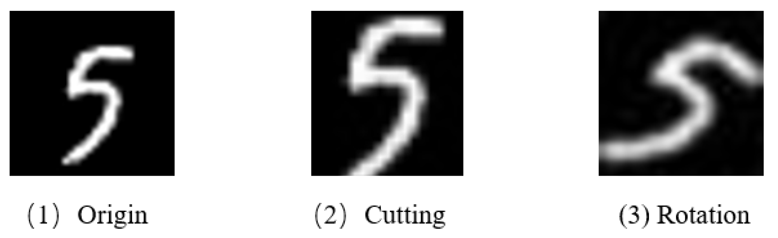
- (1)
- An encoder only clustering network structures is proposed, and PEDCC is used as the clustering center to ensure the maximum inter-class distance in latent feature space. Data distribution constraint and contrastive constraint between samples and augmented samples are applied to improve the clustering performance;
- (2)
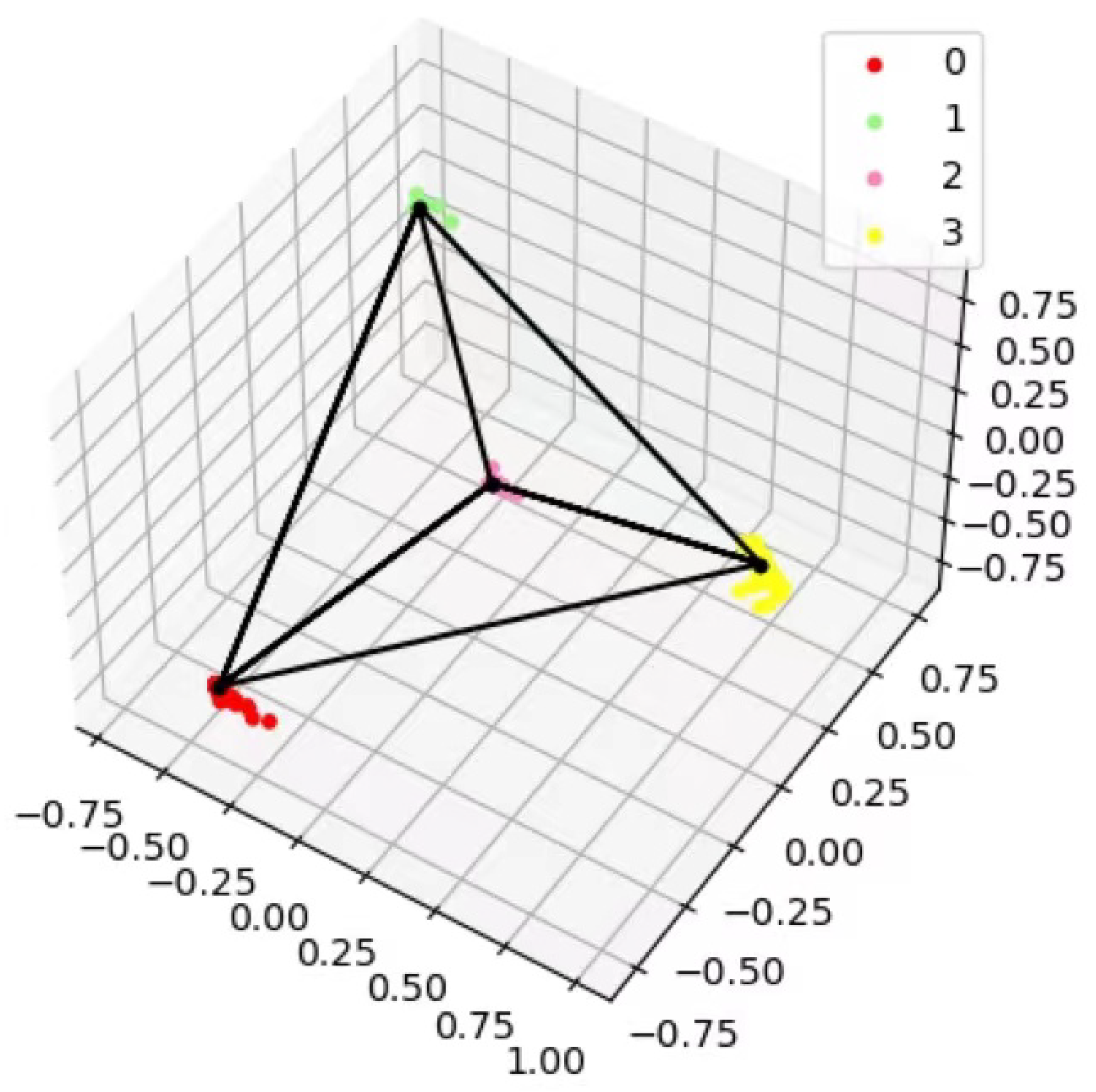
- The algorithm normalizes the latent features, and composite cosine distance is proposed to replace Euclidean distance to achieve a better clustering effect. Experiments on several public data sets show that the proposed algorithm achieves the SOTA results.
- (3)
- For complex natural images such as CIFAR-10 and STL-10, a self-supervised pretrained model can be used to effectively improve clustering performance.
2. Related Work
2.1. Clustering and Deep Learning Based Clustering Method
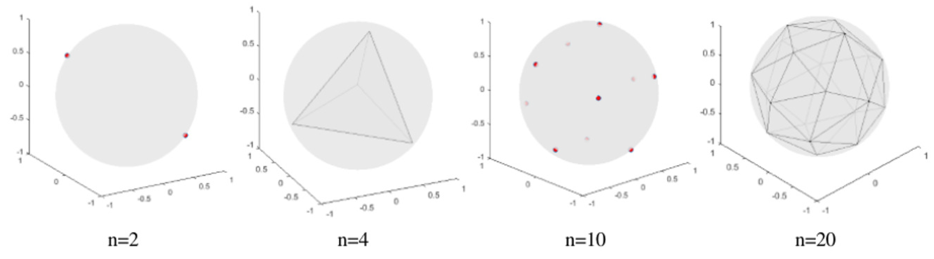
2.2. PEDCC
3. Methods
3.1. ICBPC
| Algorithm 1 ICBPC algorithm |
| Input:X = unlabeled images; |
| Output:K classes of clustering images; |
| 1: Initialize PEDCC cluster centers; |
| 2: repeat |
| 3: = Augumentation(X); |
| 4: = Encoder(); Z = Encoder(X); |
| 5: = MMD(, PEDCC); = Contrastive loss(, ); |
| 6: until Stopping criterion meet |
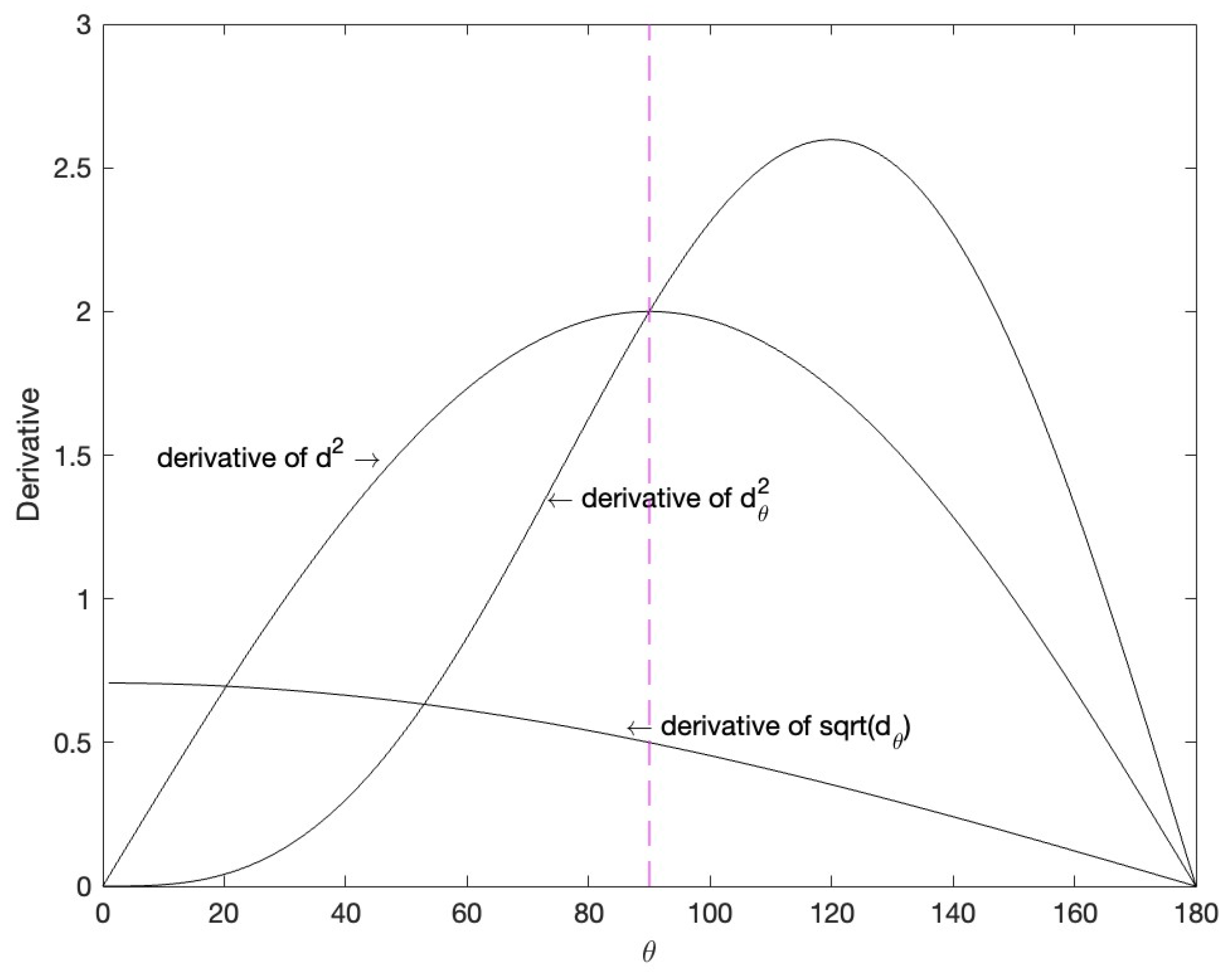
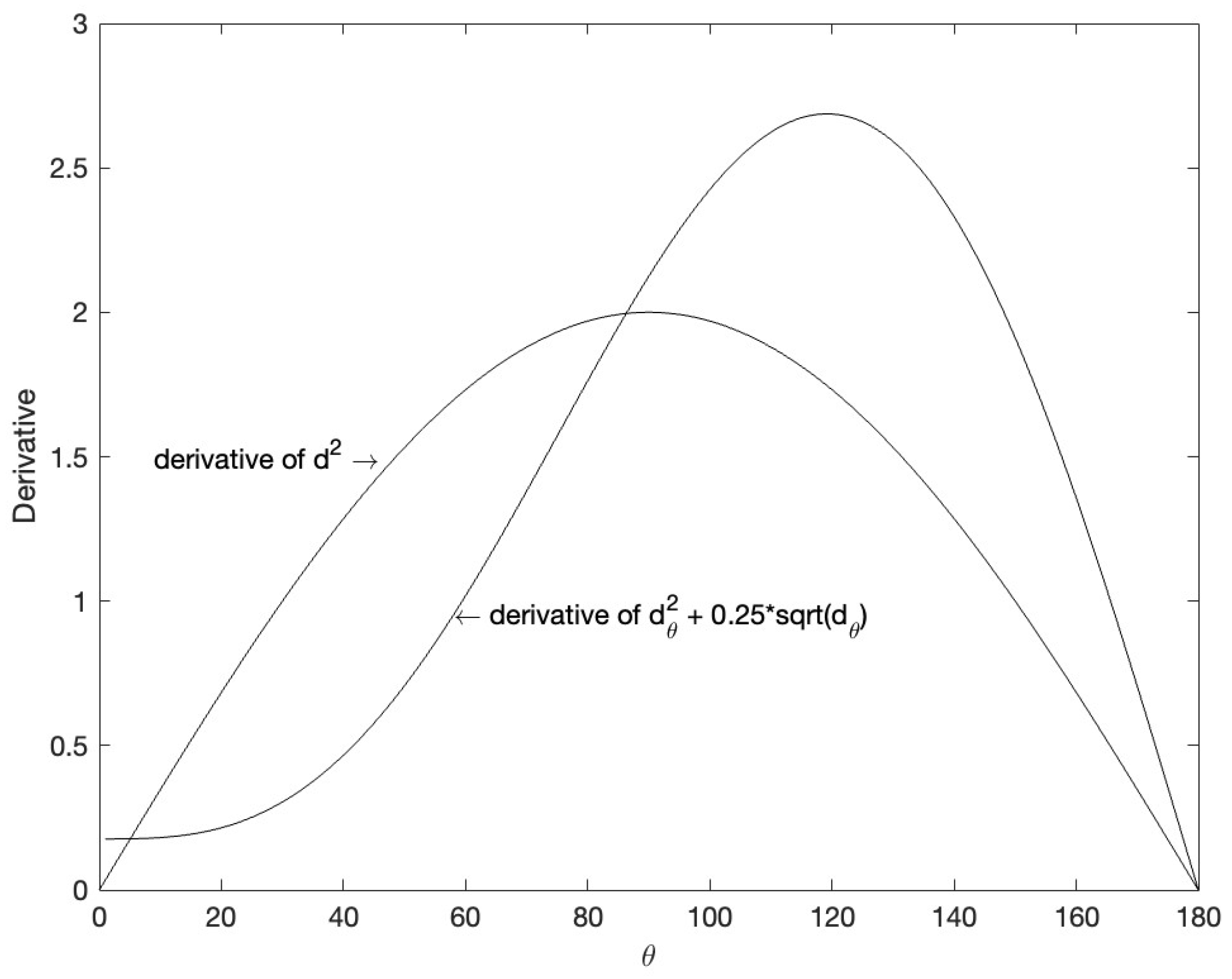
3.2. Composite Cosine Distance for Normalized Features and PEDCC
3.3. Clustering Loss Function
3.4. Data Augmentation Loss Function
3.5. Loss Function
3.6. Using Self-Supervised Pretrained Model
4. Experiments and Discussions
4.1. Experiments Settings
4.1.1. Datasets
4.1.2. Experimental Setup
4.1.3. Evaluation Metrics
4.1.4. Encoder Architecture
4.2. Analysis on Computational Time and Clustering
4.3. Ablation Experiment
4.4. Effectiveness of Self-Supervised Pretrained Model
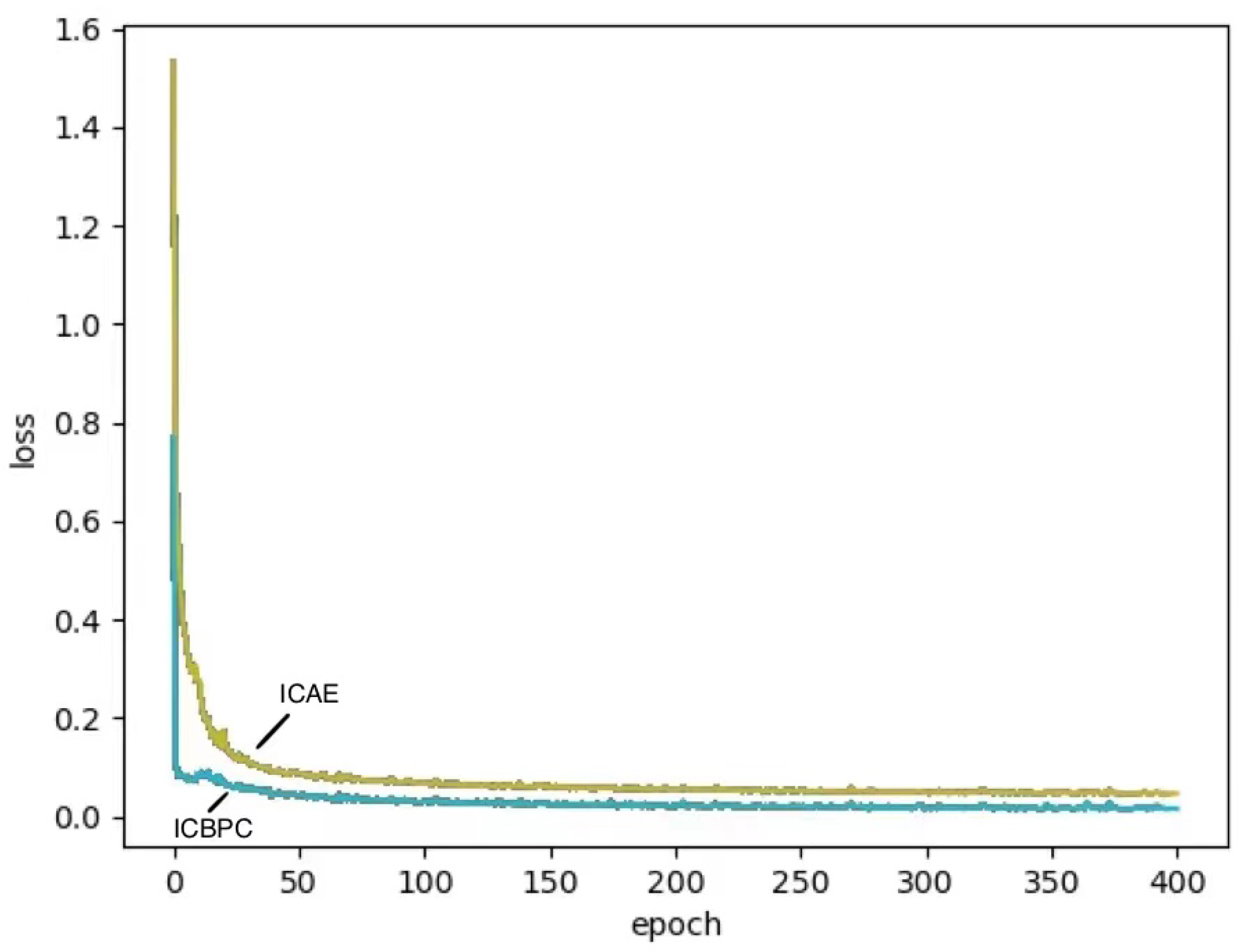
4.5. Compared with Auto-Encoder
4.6. Compared with the Latest Clustering Algorithm
4.7. Statistical Analysis of Experimental Data
5. Conclusions
Author Contributions
Funding
Institutional Review Board Statement
Informed Consent Statement
Data Availability Statement
Conflicts of Interest
References
- Zhu, Q.; Zhang, R. A Classification Supervised Auto-Encoder Based on Predefined Evenly-Distributed Class Centroids. arXiv 2019, arXiv:1902.00220. [Google Scholar]
- Zhu, Q.; Zu, X. Fully Convolutional Neural Network Structure and Its Loss Function for Image Classification. IEEE Access 2022, 10, 35541–35549. [Google Scholar] [CrossRef]
- Zhu, Q.; Zheng, G.; Shen, J.; Wang, R. Out-of-Distribution Detection Based on Feature Fusion in Neural Network Classifier Pre-Trained by PEDCC-Loss. IEEE Access 2022, 10, 66190–66197. [Google Scholar] [CrossRef]
- Hadsell, R.; Chopra, S.; Lecun, Y. Dimensionality Reduction by Learning an Invariant Mapping. In Proceedings of the 2006 IEEE Computer Society Conference on Computer Vision and Pattern Recognition (CVPR’06), New York, NY, USA, 17–22 June 2006. [Google Scholar]
- Kullback, S.; Leibler, R.A. On information and sufficiency. Ann. Math. Stat. 1951, 22, 79–86. [Google Scholar] [CrossRef]
- MacQueen, J. Some methods for classification and analysis of multivariate observations. In Proceedings of the Fifth Berkeley Symposium on Mathematical Statistics and Probability, Oakland, CA, USA, 21 June–18 July 1965; Volume 1, pp. 281–297. [Google Scholar]
- Gdalyahu, Y.; Weinshall, D.; Werman, M. Self-organization in vision: Stochastic clustering for image segmentation, perceptual grouping, and image database organization. IEEE Trans. Pattern Anal. Mach. Intell. 2001, 23, 1053–1074. [Google Scholar] [CrossRef] [Green Version]
- Krizhevsky, A.; Sutskever, I.; Hinton, G. ImageNet Classification with Deep Convolutional Neural Networks. In Proceedings of the NIPS, Lake Tahoe, NV, USA, 3–6 December 2012. [Google Scholar]
- Shao, L.; Wu, D.; Li, X. Learning Deep and Wide: A Spectral Method for Learning Deep Networks. IEEE Trans. Neural Netw. Learn. Syst. 2014, 25, 2303–2308. [Google Scholar] [CrossRef] [PubMed]
- Doersch, C. Tutorial on variational autoencoders. arXiv 2016, arXiv:1606.05908. [Google Scholar]
- Kingma, D.P.; Welling, M. Auto-encoding variational bayes. arXiv 2013, arXiv:1312.6114. [Google Scholar]
- Xie, J.; Girshick, R.; Farhadi, A. Unsupervised deep embedding for clustering analysis. In Proceedings of the International Conference on Machine Learning, New York, NY, USA, 19–24 June 2016; pp. 478–487. [Google Scholar]
- Li, F.; Qiao, H.; Zhang, B. Discriminatively boosted image clustering with fully convolutional auto-encoders. Pattern Recognit. 2018, 83, 161–173. [Google Scholar] [CrossRef] [Green Version]
- Lv, J.; Kang, Z.; Lu, X.; Xu, Z. Pseudo-supervised Deep Subspace Clustering. IEEE Trans. Image Process. 2021, 30, 5252–5263. [Google Scholar] [CrossRef] [PubMed]
- Guo, J.; Yuan, X.; Xu, P.; Bai, H.; Liu, B. Improved image clustering with deep semantic embedding. Pattern Recognit. Lett. 2020, 130, 225–233. [Google Scholar] [CrossRef]
- Yu, S.; Liu, J.; Han, Z.; Li, Y.; Tang, Y.; Wu, C. Representation Learning Based on Autoencoder and Deep Adaptive Clustering for Image Clustering. Math. Probl. Eng. 2021, 2021, 3742536. [Google Scholar] [CrossRef]
- Chang, J.; Wang, L.; Meng, G.; Xiang, S.; Pan, C. Deep adaptive image clustering. In Proceedings of the IEEE International Conference on Computer Vision, Venice, Italy, 22–29 October 2017; pp. 5879–5887. [Google Scholar]
- Haeusser, P.; Plapp, J.; Golkov, V.; Aljalbout, E.; Cremers, D. Associative deep clustering: Training a classification network with no labels. In German Conference on Pattern Recognition; Springer: Berlin/Heidelberg, Germany, 2018; pp. 18–32. [Google Scholar]
- Caron, M.; Bojanowski, P.; Joulin, A.; Douze, M. Deep clustering for unsupervised learning of visual features. In Proceedings of the European Conference on Computer Vision (ECCV), Munich, Germany, 8–14 September 2018; pp. 132–149. [Google Scholar]
- Zhu, Q.; Wang, Z. An Image Clustering Auto-Encoder Based on Predefined Evenly-Distributed Class Centroids and MMD Distance. Neural Process. Lett. 2020, 51, 1973–1988. [Google Scholar] [CrossRef]
- Gidaris, S.; Singh, P.; Komodakis, N. Unsupervised Representation Learning by Predicting Image Rotations. arXiv 2018, arXiv:1803.07728. [Google Scholar]
- Howard, A.G. Some Improvements on Deep Convolutional Neural Network Based Image Classification. arXiv 2013, arXiv:1312.5402. [Google Scholar]
- Zbontar, J.; Jing, L.; Misra, I.; LeCun, Y.; Deny, S. Barlow twins: Self-supervised learning via redundancy reduction. In Proceedings of the International Conference on Machine Learning, Virtual, 18–24 July 2021; pp. 12310–12320. [Google Scholar]
- Strehl, A.; Ghosh, J. Cluster ensembles—A knowledge reuse framework for combining multiple partitions. J. Mach. Learn. Res. 2002, 3, 583–617. [Google Scholar]
- He, K.; Zhang, X.; Ren, S.; Sun, J. Deep residual learning for image recognition. In Proceedings of the IEEE Conference on Computer Vision and Pattern Recognition, Las Vegas, NV, USA, 26 June 26–1 July 2016; pp. 770–778. [Google Scholar]
- Shi, J.; Malik, J. Normalized cuts and image segmentation. IEEE Trans. Pattern Anal. Mach. Intell. 2000, 22, 888–905. [Google Scholar]
- Chen, X.; Cai, D. Large scale spectral clustering with landmark-based representation. In Proceedings of the Twenty-Fifth AAAI Conference on Artificial Intelligence, San Francisco, CA, USA, 7–11 August 2011. [Google Scholar]
- Cai, D.; He, X.; Wang, X.; Bao, H.; Han, J. Locality preserving nonnegative matrix factorization. In Proceedings of the Twenty-First International Joint Conference on Artificial Intelligence, Pasadena, CA, USA, 14–17 July 2009. [Google Scholar]
- Zhao, D.; Tang, X. Cyclizing clusters via zeta function of a graph. In Proceedings of the Advances in Neural Information Processing Systems, Vancouver, BC, Canada, 7–10 December 2009; pp. 1953–1960. [Google Scholar]
- Zhang, W.; Wang, X.; Zhao, D.; Tang, X. Graph degree linkage: Agglomerative clustering on a directed graph. In European Conference on Computer Vision; Springer: Berlin/Heidelberg, Germany, 2012; pp. 428–441. [Google Scholar]
- Shah, S.A.; Koltun, V. Robust continuous clustering. Proc. Natl. Acad. Sci. USA 2017, 114, 9814–9819. [Google Scholar] [CrossRef] [PubMed] [Green Version]
- Yang, B.; Fu, X.; Sidiropoulos, N.D.; Hong, M. Towards k-means-friendly spaces: Simultaneous deep learning and clustering. In Proceedings of the 34th International Conference on Machine Learning, Sydney, Australia, 6–11 August 2017; Volume 70, pp. 3861–3870. [Google Scholar]
- Guo, X.; Gao, L.; Liu, X.; Yin, J. Improved deep embedded clustering with local structure preservation. In Proceedings of the IJCAI, Melbourne, Australia, 19–25 August 2017; pp. 1753–1759. [Google Scholar]
- Peng, X.; Feng, J.; Lu, J.; Yau, W.Y.; Yi, Z. Cascade subspace clustering. In Proceedings of the Thirty-First AAAI Conference on Artificial Intelligence, San Francisco, CA, USA, 4–9 February 2017. [Google Scholar]
- Jiang, Z.; Zheng, Y.; Tan, H.; Tang, B.; Zhou, H. Variational deep embedding: An unsupervised and generative approach to clustering. arXiv 2016, arXiv:1611.05148. [Google Scholar]
- Yang, J.; Parikh, D.; Batra, D. Joint unsupervised learning of deep representations and image clusters. In Proceedings of the IEEE Conference on Computer Vision and Pattern Recognition, Las Vegas, NV, USA, 26 June–1 July 2016; pp. 5147–5156. [Google Scholar]
- Ghasedi Dizaji, K.; Herandi, A.; Deng, C.; Cai, W.; Huang, H. Deep clustering via joint convolutional autoencoder embedding and relative entropy minimization. In Proceedings of the IEEE International Conference on Computer Vision, Venice, Italy, 22–29 October 2017; pp. 5736–5745. [Google Scholar]
- Hsu, C.C.; Lin, C.W. Cnn-based joint clustering and representation learning with feature drift compensation for large-scale image data. IEEE Trans. Multimed. 2017, 20, 421–429. [Google Scholar] [CrossRef]
- Huang, P.; Huang, Y.; Wang, W.; Wang, L. Deep embedding network for clustering. In Proceedings of the 2014 22nd International Conference on Pattern Recognition, Stockholm, Sweden, 24–28 August 2014; IEEE: Piscataway Township, NJ, USA, 2014; pp. 1532–1537. [Google Scholar]
- Saito, S.; Tan, R.T. Neural Clustering: Concatenating Layers for Better Projections. 2017. Available online: https://openreview.net/forum?id=r1PyAP4Yl (accessed on 29 August 2022).
- Chen, D.; Lv, J.; Zhang, Y. Unsupervised multi-manifold clustering by learning deep representation. In Proceedings of the Workshops at the Thirty-First AAAI Conference on Artificial Intelligence, San Francisco, CA, USA, 4–9 February 2017. [Google Scholar]
- Wang, Z.; Chang, S.; Zhou, J.; Wang, M.; Huang, T.S. Learning a task-specific deep architecture for clustering. In Proceedings of the 2016 SIAM International Conference on Data Mining, Miami, FL, USA, 5–7 May 2016; SIAM: Philadelphia, PA, USA, 2016; pp. 369–377. [Google Scholar]
- Hu, W.; Miyato, T.; Tokui, S.; Matsumoto, E.; Sugiyama, M. Learning discrete representations via information maximizing self-augmented training. In Proceedings of the 34th International Conference on Machine Learning, Sydney, Australia, 6–11 August 2017; Volume 70, pp. 1558–1567. [Google Scholar]


| Datasets | ||
|---|---|---|
| MNIST | 8.00 | 0.25 |
| COIL20 | 9.00 | 0.25 |
| Fashion MNIST | 8.00 | 0.25 |
| CIFAR-10 | 9.00 | 0.25 |
| STL-10 | 8.00 | 0.25 |
| ImageNet-10 | 8.00 | 0.25 |
| Datasets | Samples | Categories | Image Size |
|---|---|---|---|
| MNIST | 70,000 | 10 | 28 × 28 |
| COIL20 | 1440 | 20 | 128 × 128 |
| Fashion-MNIST | 70,000 | 10 | 28 × 28 |
| CIFAR-10 | 60,000 | 10 | 32 × 32 × 3 |
| STL-10 | 5000 | 10 | 96 × 96 × 3 |
| ImageNet-10 | 13,000 | 10 | 224 × 224 × 3 |
| Layer | Output Size | Remarks |
|---|---|---|
| Conv1 | 3232 | 32 channels |
| maxpool | 3232 | 33, stride = 2 |
| BasicBlock1 | 1616 | 64 channels |
| BasicBlock2 | 88 | 128 channels |
| BasicBlock3 | 44 | 256 channels |
| BasicBlock4 | 22 | 512 channels, Encoder output |
| Fully connected layer 1 | dimension of latent features | latent features |
| Data Sets | Dimension of Latent Features | ACC | NMI |
|---|---|---|---|
| MNIST | 40 | 0.986 | 0.979 |
| MNIST | 60 | 0.994 | 0.985 |
| MNIST | 80 | 0.989 | 0.980 |
| MNIST | 100 | 0.982 | 0.976 |
| Datasets | Dimension of Latent Features |
|---|---|
| MNIST | 60 |
| COIL20 | 160 |
| Fashion MNIST | 100 |
| CIFAR-10 | 60 |
| STL-10 | 100 |
| ImageNet-10 | 100 |
| Datasets | Composite Cosine Distance | Euclidean Distance | Normal Cosine Distance | ACC | NMI | ||
|---|---|---|---|---|---|---|---|
| MNIST | ✓ | ✓ | 0.398 | 0.312 | |||
| MNIST | ✓ | ✓ | ✓ | 0.994 | 0.985 | ||
| MNIST | ✓ | ✓ | ✓ | 0.981 | 0.961 | ||
| MNIST | ✓ | ✓ | ✓ | 0.982 | 0.965 | ||
| Fashion-MNIST | ✓ | ✓ | 0.467 | 0.354 | |||
| Fashion-MNIST | ✓ | ✓ | ✓ | 0.737 | 0.714 | ||
| Fashion-MNIST | ✓ | ✓ | ✓ | 0.725 | 0.699 | ||
| Fashion-MNIST | ✓ | ✓ | ✓ | 0.722 | 0.693 | ||
| COIL20 | ✓ | ✓ | 0.410 | 0.561 | |||
| COIL20 | ✓ | ✓ | ✓ | 0.960 | 0.982 | ||
| COIL20 | ✓ | ✓ | ✓ | 0.920 | 0.960 | ||
| COIL20 | ✓ | ✓ | ✓ | 0.920 | 0.958 | ||
| CIFAR-10 | ✓ | ✓ | 0.124 | 0.113 | |||
| CIFAR-10 | ✓ | ✓ | ✓ | 0.298 | 0.182 | ||
| CIFAR-10 | ✓ | ✓ | ✓ | 0.278 | 0.172 | ||
| CIFAR-10 | ✓ | ✓ | ✓ | 0.273 | 0.163 | ||
| STL-10 | ✓ | ✓ | 0.186 | 0.157 | |||
| STL-10 | ✓ | ✓ | ✓ | 0.551 | 0.525 | ||
| STL-10 | ✓ | ✓ | ✓ | 0.535 | 0.519 | ||
| STL-10 | ✓ | ✓ | ✓ | 0.540 | 0.522 | ||
| ImageNet-10 | ✓ | ✓ | 0.152 | 0.234 | |||
| ImageNet-10 | ✓ | ✓ | ✓ | 0.412 | 0.375 | ||
| ImageNet-10 | ✓ | ✓ | ✓ | 0.401 | 0.349 | ||
| ImageNet-10 | ✓ | ✓ | ✓ | 0.405 | 0.356 |
| Datasets | Without Pretrained | Pretrained | ACC | NMI |
|---|---|---|---|---|
| Fashion-MNIST | ✓ | 0.714 | 0.737 | |
| Fashion-MNIST | ✓ | 0.712 | 0.732 | |
| CIFAR-10 | ✓ | 0.241 | 0.125 | |
| CIFAR-10 | ✓ | 0.298 | 0.182 | |
| STL-10 | ✓ | 0.293 | 0.205 | |
| STL-10 | ✓ | 0.551 | 0.525 | |
| ImageNet-10 | ✓ | 0.250 | 0.193 | |
| ImageNet-10 | ✓ | 0.412 | 0.375 |
| Datasets | Encoder-Only | Auto-Encoder | Training Time of Each Epoch (s) | ACC | NMI |
|---|---|---|---|---|---|
| MNIST | ✓ | 58 | 0.988 | 0.965 | |
| MNIST | ✓ | 40 | 0.994 | 0.985 | |
| Fashion-MNIST | ✓ | 122 | 0.689 | 0.731 | |
| Fashion-MNIST | ✓ | 75 | 0.714 | 0.737 | |
| COIL20 | ✓ | 29 | 0.920 | 0.953 | |
| COIL20 | ✓ | 14 | 0.960 | 0.982 | |
| CIFAR-10 | ✓ | 132 | 0.284 | 0.163 | |
| CIFAR-10 | ✓ | 98 | 0.298 | 0.182 | |
| STL-10 | ✓ | 86 | 0.532 | 0.521 | |
| STL-10 | ✓ | 66 | 0.551 | 0.525 | |
| ImageNet-10 | ✓ | 205 | 0.407 | 0.365 | |
| ImageNet-10 | ✓ | 130 | 0.412 | 0.375 |
| - | ARCH | NMI | ACC | NMI | ACC | NMI | ACC | NMI | ACC | NMI | ACC | NMI | ACC |
|---|---|---|---|---|---|---|---|---|---|---|---|---|---|
| - | - | mnist | mnist | coil20 | coil20 | fashion | fashion | cifar-10 | cifar-10 | stl-10 | stl-10 | image-net-10 | image-net-10 |
| k-means [6] | - | 0.500 | 0.532 | - | - | 0.512 | 0.474 | 0.064 | 0.199 | 0.125 | 0.192 | - | - |
| SC-NCUT [26] | - | 0.731 | 0.656 | - | - | 0.575 | 0.508 | - | - | - | - | - | - |
| SC-LS [27] | - | 0.706 | 0.714 | - | - | 0.497 | 0.496 | - | - | - | - | - | - |
| NMF-LP [28] | - | 0.452 | 0.471 | - | - | 0.425 | 0.434 | 0.051 | 0.180 | - | - | - | - |
| AC-Zell [29] | - | 0.017 | 0.113 | - | - | 0.100 | 0.010 | - | - | - | - | - | - |
| AC-GDL [30] | - | 0.017 | 0.113 | - | - | 0.010 | 0.112 | - | - | - | - | - | - |
| RCC [31] | - | 0.893 | - | - | - | - | - | - | - | - | - | ||
| DCN [32] | MLP | 0.810 | 0.830 | - | - | 0.558 | 0.501 | - | - | - | - | ||
| DEC [12] | MLP | 0.834 | 0.863 | - | - | 0.546 | 0.518 | 0.057 | 0.208 | 0.276 | 0.359 | ||
| IDEC [33] | - | 0.867 | 0.881 | - | - | 0.557 | 0.529 | - | - | - | - | - | - |
| CSC [34] | - | 0.755 | 0.872 | - | - | - | - | - | - | - | - | - | - |
| VADE [35] | VAE | 0.876 | 0.945 | - | - | 0.630 | 0.578 | - | - | - | - | - | - |
| JULE [36] | CNN | 0.913 | 0.964 | - | - | 0.608 | 0.563 | - | - | 0.182 | 0.277 | - | - |
| DBC [13] | CNN | 0.917 | 0.964 | - | - | - | - | - | - | - | - | - | - |
| DEPICT [37] | CNN | 0.917 | 0.965 | - | - | 0.392 | 0.392 | - | - | - | - | - | - |
| CCNN [38] | CNN | 0.876 | - | - | - | - | - | - | - | - | - | - | - |
| DEN [39] | MLP | - | - | 0.870 | 0.724 | - | - | - | - | - | - | - | - |
| NC [40] | MLP | - | 0.966 | - | - | - | - | - | - | - | - | - | - |
| UMMC [41] | DBN | 0.864 | - | 0.891 | - | - | - | - | - | - | - | - | - |
| TAGNET [42] | - | 0.651 | 0.692 | 0.927 | 0.899 | - | - | - | - | - | - | - | - |
| IMSAT [43] | MLP | - | 0.983 | - | - | - | - | - | - | - | - | - | - |
| PSSC [14] | AE | 0.768 | 0.843 | 0.978 | 0.972 | - | - | - | - | - | - | - | - |
| DAC [17] | - | 0.935 | 0.978 | - | - | - | - | 0.396 | 0.522 | 0.366 | 0.469 | - | - |
| ADC [18] | - | - | 0.987 | - | - | - | - | - | 0.293 | - | - | - | - |
| ICAE [20] | AE | 0.967 | 0.988 | 0.953 | 0.920 | 0.689 | 0.731 | 0.080 | 0.215 | - | - | - | - |
| ICBPC(ours) | - | 0.985 | 0.994 | 0.982 | 0.960 | 0.714 | 0.737 | 0.182 | 0.298 | 0.525 | 0.551 | 0.412 | 0.375 |
| Datasets | Average of ACC | Average of NMI | Standard Deviation of ACC | Standard Deviation of NMI |
|---|---|---|---|---|
| MNIST | 0.994 | 0.985 | 0.0048 | 0.0034 |
| COIL20 | 0.960 | 0.982 | 0.0005 | 0.0013 |
| Fashion MNIST | 0.737 | 0.714 | 0.0036 | 0.0041 |
| CIFAR-10 | 0.298 | 0.182 | 0.0045 | 0.0032 |
| STL-10 | 0.551 | 0.525 | 0.0062 | 0.0053 |
| ImageNet-10 | 0.412 | 0.375 | 0.0064 | 0.0055 |
Publisher’s Note: MDPI stays neutral with regard to jurisdictional claims in published maps and institutional affiliations. |
© 2022 by the authors. Licensee MDPI, Basel, Switzerland. This article is an open access article distributed under the terms and conditions of the Creative Commons Attribution (CC BY) license (https://creativecommons.org/licenses/by/4.0/).
Share and Cite
Zhu, Q.; Hu, L.; Wang, R. Image Clustering Algorithm Based on Predefined Evenly-Distributed Class Centroids and Composite Cosine Distance. Entropy 2022, 24, 1533. https://doi.org/10.3390/e24111533
Zhu Q, Hu L, Wang R. Image Clustering Algorithm Based on Predefined Evenly-Distributed Class Centroids and Composite Cosine Distance. Entropy. 2022; 24(11):1533. https://doi.org/10.3390/e24111533
Chicago/Turabian StyleZhu, Qiuyu, Liheng Hu, and Rui Wang. 2022. "Image Clustering Algorithm Based on Predefined Evenly-Distributed Class Centroids and Composite Cosine Distance" Entropy 24, no. 11: 1533. https://doi.org/10.3390/e24111533