
Efficient Power Characteristic Analysis and Multi-Objective Optimization for an Irreversible Simple Closed Gas Turbine Cycle


Abstract
:1. Introduction
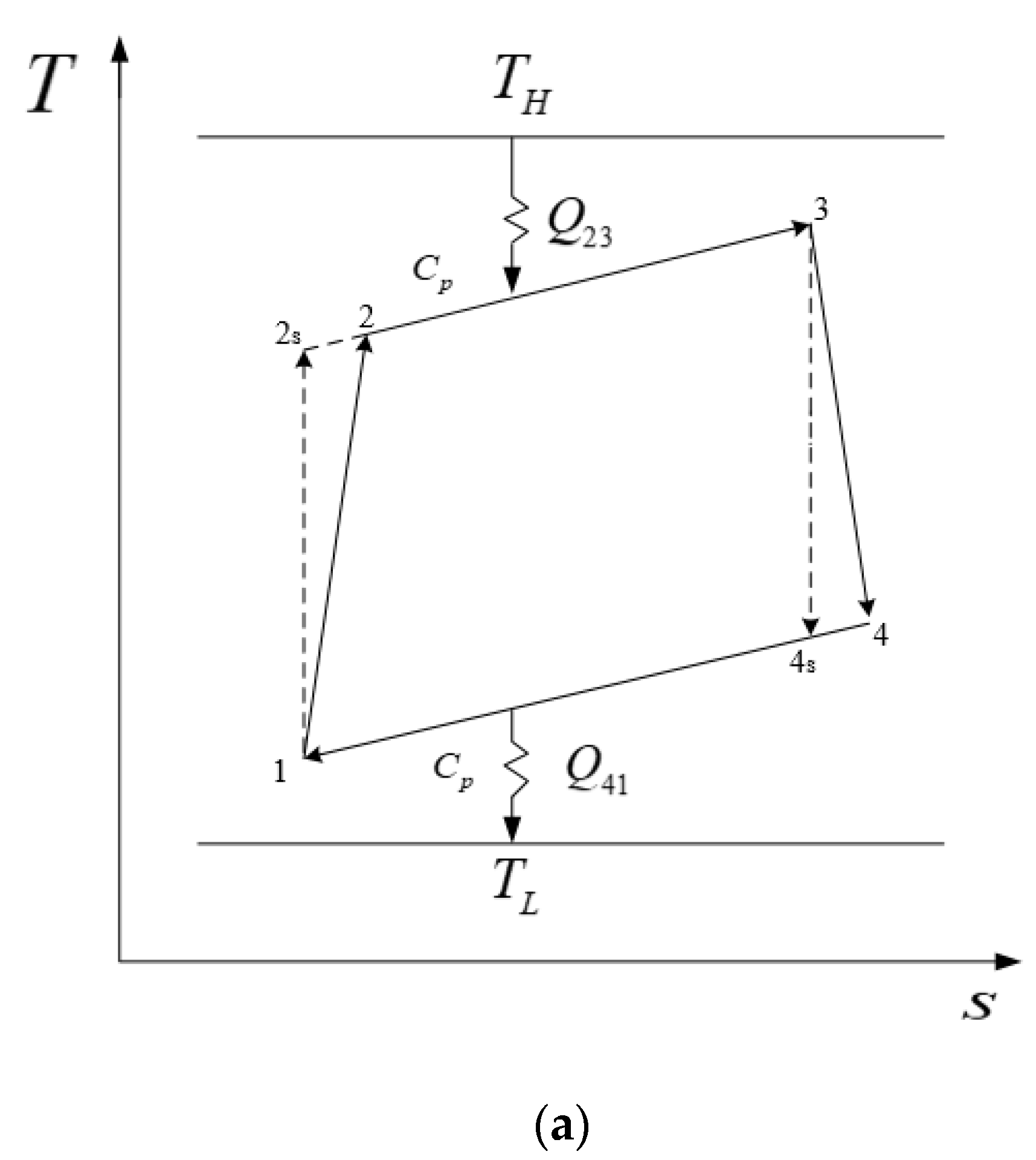
2. Cycle Model
3. Efficient Power Performance Analyses
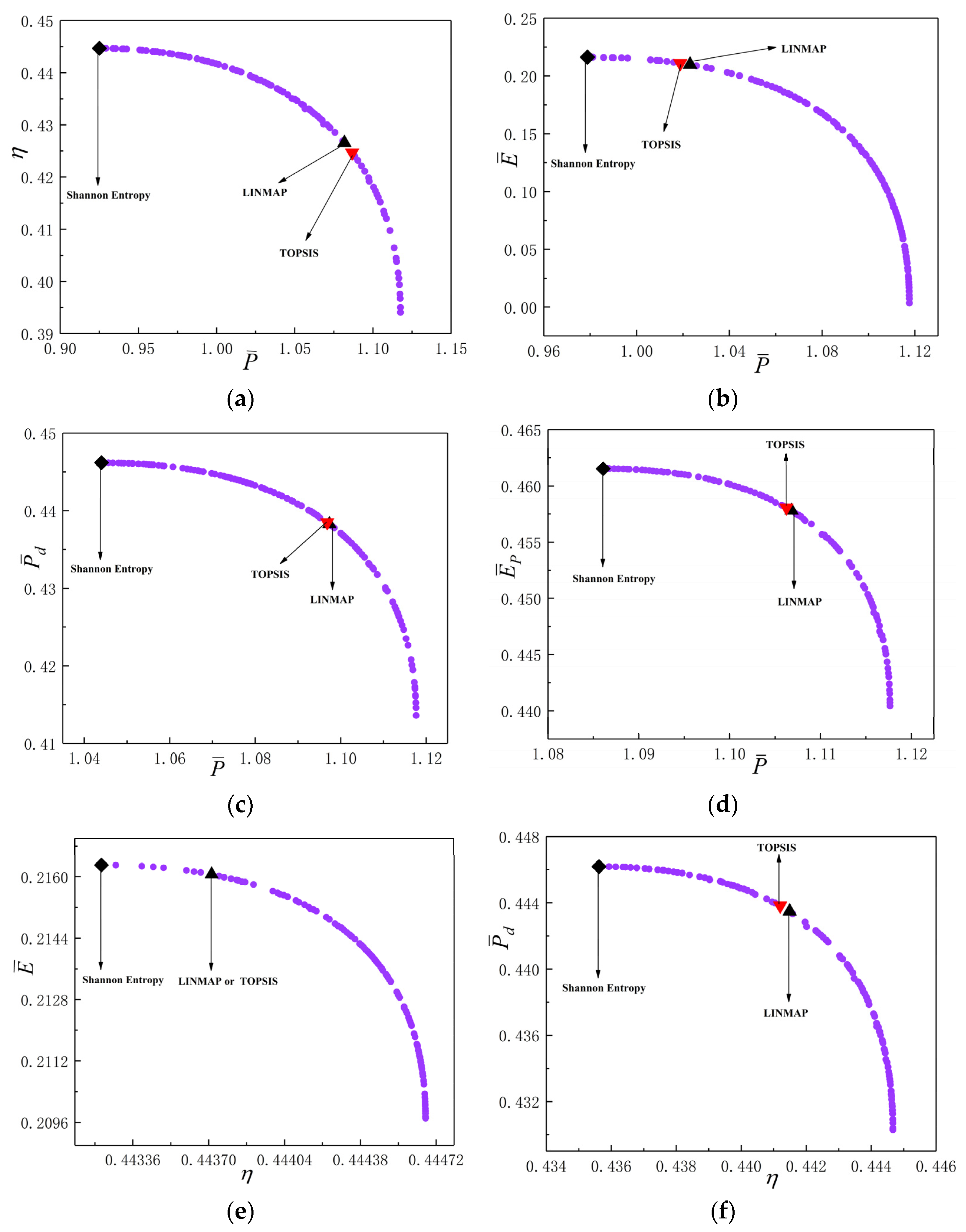
4. Multi-Objective Optimizations
5. Conclusions
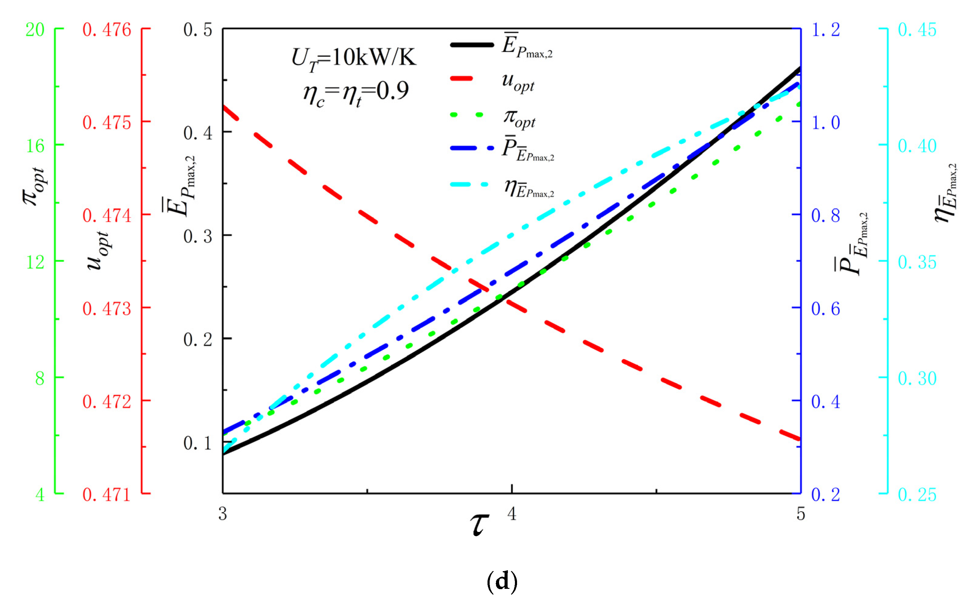
- When the is constant, the existence of both and make cycle reach a quadratic maximum (); with the raises of , , and , cycle has a significant raise, of which and have great impacts on .
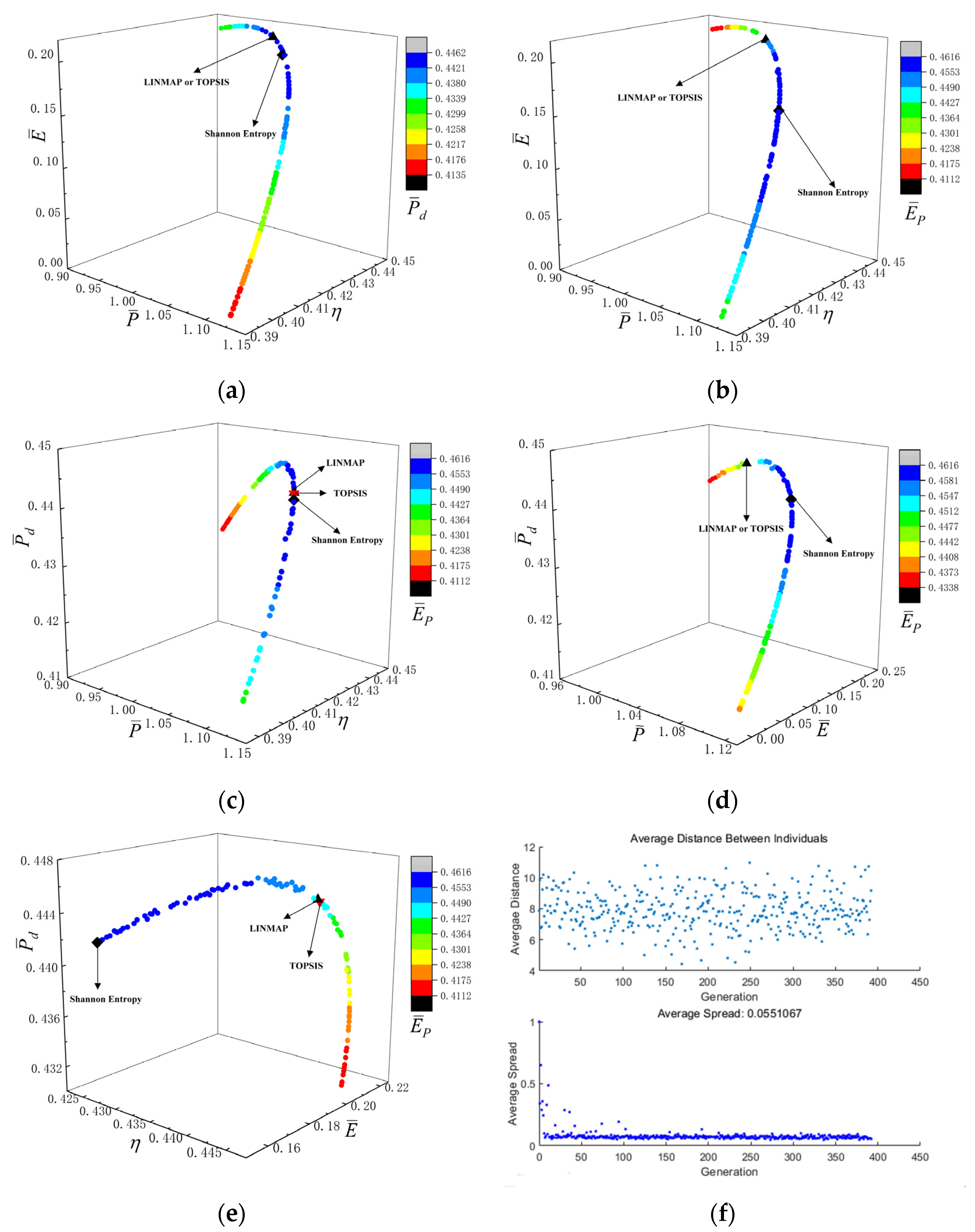
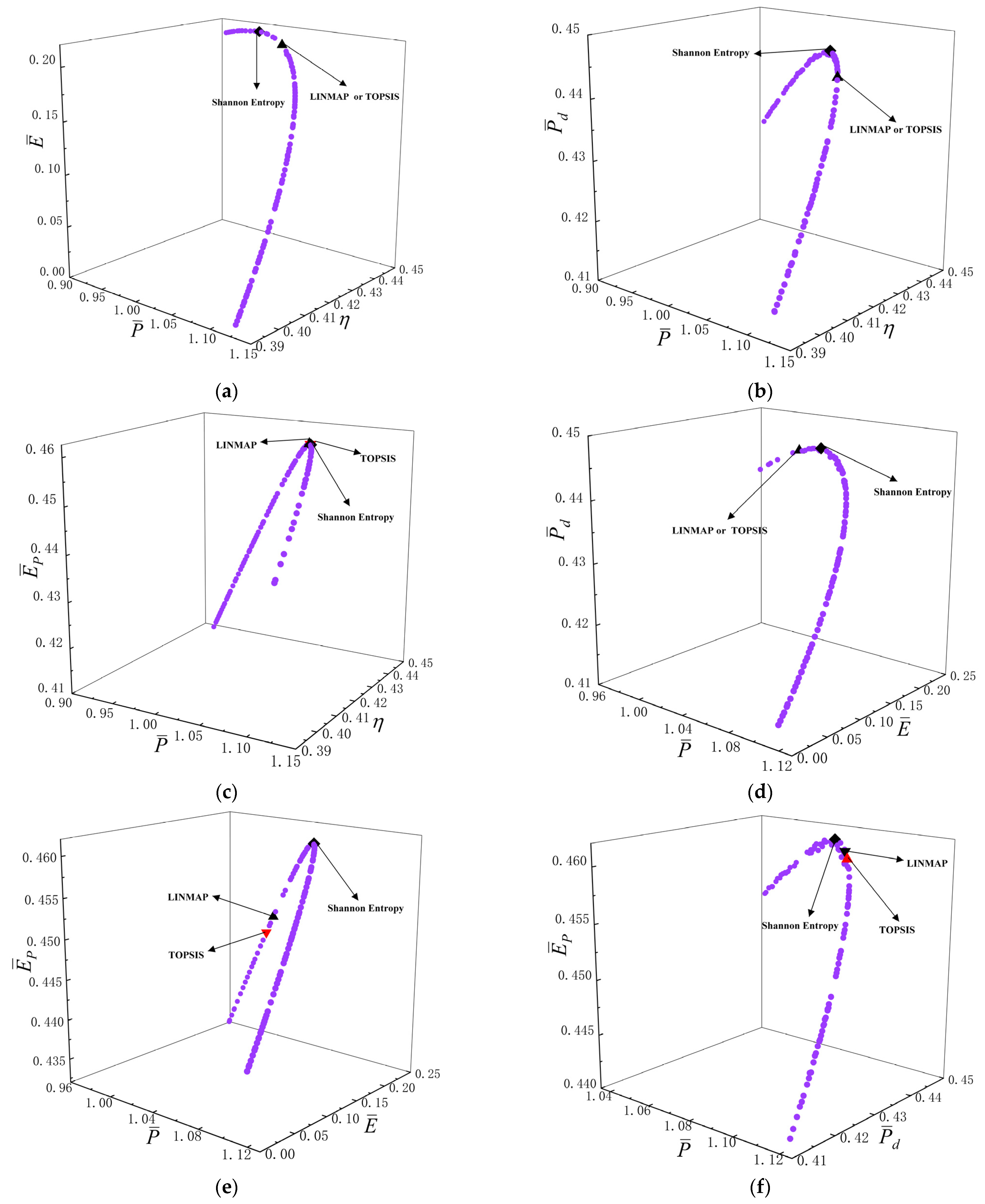
- For five-objective optimization, the obtained by the Shannon Entropy decision-making method is 0.2284, which is better than other decision-making methods.
- For four-objective combination optimizations, the obtained by LINMAP decision-making method with four-objective optimization of , , and is 0.2163, which is better than other four-objective combination optimizations.
- For three-objective combination optimizations, the obtained by LINMAP decision-making method with three-objective optimization of , and is 0.2067, which is better than other three-objective combination optimizations.
- For two-objective combination optimization, the obtained by LINMAP decision-making method with two-objective optimization of and is 0.2060, which is better than other two-objective combination optimizations.
- FTT and NSGA-II are powerful theoretical and computational tools for comprehensive performance optimization of a simple irreversible CGT cycle.
Author Contributions
Funding
Institutional Review Board Statement
Data Availability Statement
Acknowledgments
Conflicts of Interest
Nomenclature
| Thermal capacity ratio () | |
| Deviation index | |
| Effectiveness of heat exchanger or ecological function () | |
| Efficient power () | |
| Specific heat ratio | |
| Number of the heat transfer unit | |
| Power output () | |
| Power density () | |
| Pressure () | |
| Heat absorbing rate or heat releasing rate () | |
| Entropy production rate () | |
| Temperature () | |
| Ambient temperature () | |
| Heat conductance () | |
| Total heat conductance () | |
| Distribution of hot-side heat exchanger heat conductance | |
| Volume () | |
| Greek symbols | |
| Thermal efficiency | |
| Pressure ratio | |
| Heat reservoirs temperature ratio | |
| Subscripts | |
| Compressor | |
| Double maximum dimensionless efficient power point | |
| Hot-side | |
| Cold-side | |
| Maximum value | |
| Double maximum value | |
| Optimal | |
| Maximum dimensionless power point | |
| Turbine | |
| Working fluid | |
| 1–4, , | Cycle state points |
| Superscripts | |
| Dimensionless | |
| Abbreviations | |
| CGT | Closed gas turbine |
| FTT | Finite-time thermodynamic |
| HEG | Heat engine |
| HEX | Heat exchanger |
| HTC | Heat conductance |
| MOO | Multi-objective optimization |
| OO | Optimization objective |
References
- Andresen, B. Finite-Time Thermodynamics; Physics Laboratory II; University of Copenhagen: Copenhagen, Denmark, 1983. [Google Scholar]
- Chen, L.G.; Wu, C.; Sun, F.R. Finite time thermodynamic optimization or entropy generation minimization of energy systems. J. Non-Equilib. Thermodyn. 1999, 24, 327–359. [Google Scholar]
- Andresen, B. Current trends in finite-time thermodynamics. Angew. Chem. Int. Edit. 2011, 50, 2690–2704. [Google Scholar] [CrossRef] [PubMed]
- Berry, R.S.; Salamon, P.; Andresen, B. How it all began. Entropy 2020, 22, 908. [Google Scholar] [CrossRef] [PubMed]
- Andresen, B.; Salamon, P. Future perspectives of finite-time thermodynamics. Entropy 2022, 24, 690. [Google Scholar] [CrossRef]
- Chen, Y.R. Maximum profit configurations of commercial engines. Entropy 2011, 13, 1137–1151. [Google Scholar] [CrossRef] [Green Version]
- Ebrahimi, R. A new design method for maximizing the work output of cycles in reciprocating internal combustion engines. Energy Convers. Manag. 2018, 172, 164–172. [Google Scholar] [CrossRef]
- Chen, L.G.; Ma, K.; Feng, H.J.; Ge, Y.L. Optimal configuration of a gas expansion process in a piston-type cylinder with generalized convective heat transfer law. Energies 2020, 13, 3229. [Google Scholar] [CrossRef]
- Boikov, S.Y.; Andresen, B.; Akhremenkov, A.A.; Tsirlin, A.M. Evaluation of irreversibility and optimal organization of an integrated multi-stream heat exchange system. J. Non-Equilib. Thermodyn. 2020, 45, 155–171. [Google Scholar] [CrossRef]
- Masser, R.; Hoffmann, K.H. Optimal control for a hydraulic recuperation system using endoreversible thermodynamics. Appl. Sci. 2021, 11, 5001. [Google Scholar] [CrossRef]
- Scheunert, M.; Masser, R.; Khodja, A.; Paul, R.; Schwalbe, K.; Fischer, A.; Hoffmann, K.H. Power-optimized sinusoidal piston motion and its performance gain for an Alpha-type Stirling engine with limited regeneration. Energies 2020, 13, 4564. [Google Scholar] [CrossRef]
- Paul, R.; Hoffmann, K.H. Cyclic control optimization algorithm for Stirling engines. Symmetry 2021, 13, 873. [Google Scholar] [CrossRef]
- Khodja, A.; Paul, R.; Fischer, A.; Hoffmann, K.H. Optimized cooling power of a Vuilleumier refrigerator with limited regeneration. Energies 2021, 14, 8376. [Google Scholar] [CrossRef]
- Paul, R.; Hoffmann, K.H. Optimizing the piston paths of Stirling cycle cryocoolers. J. Non-Equilib. Thermodyn. 2022, 47, 195–203. [Google Scholar] [CrossRef]
- Fischer, A.; Khodja, A.; Paul, R.; Hoffmann, K.H. Heat-only-driven Vuilleumier refrigeration. Appl. Sci. 2022, 12, 1775. [Google Scholar] [CrossRef]
- Li, P.L.; Chen, L.G.; Xia, S.J.; Kong, R.; Ge, Y.L. Total entropy generation rate minimization configuration of a membrane reactor of methanol synthesis via carbon dioxide hydrogenation. Sci. China Technol. Sci. 2022, 65, 657–678. [Google Scholar] [CrossRef]
- Li, J.; Chen, L.G. Optimal configuration of finite source heat engine cycle for maximum output work with complex heat transfer law. J. Non-Equilib. Thermodyn. 2022, 47, 433–441. [Google Scholar] [CrossRef]
- Chen, L.G.; Xia, S.J. Heat engine cycle configurations for maximum work output with generalized models of reservoir thermal capacity and heat resistance. J. Non-Equilib. Thermodyn. 2022, 47, 329–338. [Google Scholar] [CrossRef]
- Ahmadi, M.H.; Pourkiaei, S.M.; Ghazvini, M.; Pourfayaz, F. Thermodynamic assessment and optimization of performance of irreversible Atkinson cycle. Iran. J. Chem. Chem. Eng. 2020, 39, 267–280. [Google Scholar]
- Shi, S.S.; Ge, Y.L.; Chen, L.G.; Feng, F.J. Four objective optimization of irreversible Atkinson cycle based on NSGA-II. Entropy 2020, 22, 1150. [Google Scholar] [CrossRef]
- Smith, Z.; Pal, P.S.; Deffner, S. Endoreversible Otto engines at maximal power. J. Non-Equilib. Thermodyn. 2020, 45, 305–310. [Google Scholar] [CrossRef]
- Insinga, A.R. The quantum friction and optimal finite-time performance of the quantum Otto cycle. Entropy 2020, 22, 1060. [Google Scholar] [CrossRef] [PubMed]
- Tang, C.Q.; Chen, L.G.; Feng, H.J.; Wang, W.H.; Ge, Y.L. Power optimization of a modified closed binary Brayton cycle with two isothermal heating processes and coupled to variable-temperature reservoirs. Energies 2020, 13, 3212. [Google Scholar] [CrossRef]
- Kim, S.J.; Kim, M.S.; Kim, M. Parametric study and optimization of closed Brayton power cycle considering the charge amount of working fluid. Energy 2020, 198, 117353. [Google Scholar] [CrossRef]
- Petrescu, S.; Harman, C.; Bejan, A.; Costea, M.; Dobre, C. Carnot cycle with external and internal irreversibilities analyzed in thermodynamics with finite speed with the direct method. Termotehnica 2011, 15, 7–17. [Google Scholar]
- Liu, X.W.; Chen, L.G.; Ge, Y.L.; Feng, H.J.; Wu, F.; Lorenzini, G. Exergy-based ecological optimization of an irreversible quantum Carnot heat pump with spin-1/2 systems. J. Non-Equilib. Thermodyn. 2021, 46, 61–76. [Google Scholar] [CrossRef]
- Wang, T.; Ge, Y.L.; Chen, L.G.; Feng, H.J.; Yu, J.Y. Optimal heat exchanger area distribution and low-temperature heat sink temperature for power optimization of an endoreversible space Carnot cycle. Entropy 2021, 23, 1285. [Google Scholar] [CrossRef]
- Ahmadi, M.A.; Pourfayaz, F.; Açıkkalp, E. Thermodynamic analysis and optimization of an irreversible nano scale dual cycle operating with Maxwell-Boltzmann gas. Mech. Ind. 2017, 18, 212. [Google Scholar] [CrossRef]
- Ge, Y.L.; Shi, S.S.; Chen, L.G.; Zhang, D.F.; Feng, H.J. Power density analysis and multi-objective optimization for an irreversible Dual cycle. J. Non-Equilib. Thermodyn. 2022, 47, 289–309. [Google Scholar] [CrossRef]
- Ahmadi, M.H.; Mohammadi, A.H.; Dehghani, S. Evaluation of the maximized power of a regenerative endoreversible Stirling cycle using the thermodynamic analysis. Energy Convers. Manag. 2013, 76, 561–570. [Google Scholar] [CrossRef]
- Lai, H.Y.; Li, Y.T.; Chan, Y.H. Efficiency enhancement on hybrid power system composed of irreversible solid oxide fuel cell and Stirling engine by finite time thermodynamics. Energies 2021, 14, 1037. [Google Scholar] [CrossRef]
- Qi, C.Z.; Ding, Z.M.; Chen, L.G.; Ge, Y.L.; Feng, H.J. Modelling of irreversible two-stage combined thermal Brownian refrigerators and their optimal performance. J. Non-Equilib. Thermodyn. 2021, 46, 175–189. [Google Scholar] [CrossRef]
- Chen, L.G.; Qi, C.Z.; Ge, Y.L.; Feng, H.J. Thermal Brownian heat engine with external and internal irreversibilities. Energy 2022, 255, 124582. [Google Scholar] [CrossRef]
- Qi, C.Z.; Chen, L.G.; Ge, Y.L.; Huang, L.; Feng, H.J. Thermal Brownian refrigerator with external and internal irreversibilities. Case Stud. Therm. Eng. 2022, 36, 102185. [Google Scholar] [CrossRef]
- Zang, P.C.; Chen, L.G.; Ge, Y.L. Maximizing Efficient Power for an Irreversible Porous Medium Cycle with Nonlinear Variation of Working Fluid’s Specific Heat. Energies 2022, 15, 6946. [Google Scholar] [CrossRef]
- Levario-Medina, S.; Valencia-Ortega, G.; Barranco-Jimenez, M.A. Energetic optimization considering a generalization of the ecological criterion in traditional simple-cycle and combined cycle power plants. J. Non-Equilib. Thermodyn. 2020, 45, 269–290. [Google Scholar] [CrossRef]
- Cao, Y.; Li, P.Y.; Qiao, Z.L.; Ren, S.J.; Si, F.Q. A concept of a supercritical CO2 Brayton and organic Rankine combined cycle for solar energy utilization with typical geothermal as auxiliary heat source: Thermodynamic analysis and optimization. Energy Rep. 2022, 8, 322–333. [Google Scholar] [CrossRef]
- Salamon, P.; Nitzon, A. Finite time optimization of a Newton’s law Carnot cycle. J. Chem. Phys. 1981, 74, 3546–3560. [Google Scholar] [CrossRef]
- Sahin, B.; Kodal, A.; Yavuz, H. Efficiency of a Joule-Brayton engine at maximum power density. J. Phys. D Appl. Phys. 1995, 28, 1309–1313. [Google Scholar] [CrossRef]
- Angulo-Brown, F. An ecological optimization criterion for finite-time heat engines. J. Appl. Phys. 1991, 69, 7465–7469. [Google Scholar] [CrossRef]
- Yan, Z.J. η and P of a Carnot engine at maximum ηP. Chin. J. Nat. 1984, 7, 475. (In Chinese) [Google Scholar]
- Yilmaz, T. A new performance criterion for heat engines: Efficient power. J. Energy Inst. 2006, 79, 38–41. [Google Scholar] [CrossRef]
- Wu, C. Power optimization of an endoreversible Brayton gas turbine heat engine. Energy Convers. Manag. 1991, 31, 561–565. [Google Scholar] [CrossRef]
- Ibrahim, O.M.; Klein, S.A.; Mitchell, J.W. Optimal heat power cycles for specified boundary conditions. Trans. ASME J. Gas Turbines Power 1991, 113, 514–521. [Google Scholar] [CrossRef]
- Wu, C.; Kiang, R.L. Power performance of a nonisentropic Brayton cycle. J. Eng. Gas Turbines Power 1991, 113, 501–504. [Google Scholar] [CrossRef]
- Chen, L.G.; Sun, F.R.; Wu, C. Performance analysis of an irreversible Brayton heat engine. J. Inst. Energy 1997, 70, 2–8. [Google Scholar]
- Cheng, C.Y.; Chen, C.K. Power optimization of an irreversible Brayton heat engine. Energy Sources 1997, 19, 461–474. [Google Scholar] [CrossRef]
- Cheng, C.Y.; Chen, C.K. Efficiency optimizations of an irreversible Brayton heat Engine. J. Energy Res. Technol. 1998, 120, 143–148. [Google Scholar] [CrossRef]
- Cheng, C.Y.; Chen, C.K. Ecological optimization of an endoreversible Brayton cycle. Energy Convers. Manag. 1998, 39, 33–34. [Google Scholar] [CrossRef]
- Ust, Y.; Sahin, B.; Kodal, A. Performance analysis of an irreversible Brayton heat engine based on ecological coefficient of performance criterion. Int. J. Therm. Sci. 2006, 45, 94–101. [Google Scholar] [CrossRef]
- Chen, L.G.; Zheng, J.L.; Sun, F.R.; Wu, C. Optimum distribution of heat exchanger inventory for power density optimization of an endoreversible closed Brayton cycle. J. Phys. D Appl. Phys. 2001, 34, 422–427. [Google Scholar] [CrossRef]
- Chen, L.G.; Zheng, J.L.; Sun, F.R.; Wu, C. Power density optimization for an irreversible closed Brayton cycle. Open Sys. Inf. Dyn. 2001, 8, 241–260. [Google Scholar] [CrossRef]
- Arora, R.; Kaushik, S.C.; Kumar, R. Performance analysis of Brayton heat engine at maximum efficient power using temperature dependent specific heat of working fluid. J. Therm. Eng. 2015, 1, 345–354. [Google Scholar]
- Radcenco, V.; Vargas, J.V.C.; Bejan, A. Thermodynamics optimization of a gas turbine power plant with pressure drop irreversibilities. Trans. ASME J. Energy Res. Technol. 1998, 120, 233–240. [Google Scholar] [CrossRef]
- Chen, L.G.; Shen, J.F.; Ge, Y.L.; Wu, Z.X.; Wang, W.H.; Zhu, F.L.; Feng, H.J. Power and efficiency optimization of open Maisotsenko-Brayton cycle and performance comparison with traditional open regenerated Brayton cycle. Energy Convers. Manag. 2020, 217, 113001. [Google Scholar] [CrossRef]
- Chen, L.G.; Yang, B.; Feng, H.J.; Ge, Y.L.; Xia, S.J. Performance optimization of an open simple-cycle gas turbine combined cooling, heating and power plant driven by basic oxygen furnace gas in China’s steelmaking plants. Energy 2020, 203, 117791. [Google Scholar] [CrossRef]
- Chen, L.G.; Feng, H.J.; Ge, Y.L. Power and efficiency optimization for open combined regenerative Brayton and inverse Brayton cycles with regeneration before the inverse cycle. Entropy 2020, 22, 677. [Google Scholar] [CrossRef] [PubMed]
- Ahmadi, M.H.; Ahmadi, M.A.; Pourfayaz, F.; Hosseinzade, H.; Acıkkalp, E.; Tlili, I.; Feidt, M. Designing a powered combined Otto and Stirling cycle power plant through multi-objective optimization approach. Renew. Sustain. Energy Rev. 2016, 62, 585–595. [Google Scholar] [CrossRef]
- Zang, P.C.; Ge, Y.L.; Chen, L.G.; Gong, Q.R. Power density characteristic analysis and multi-objective optimization of an irreversible porous medium engine cycle. Case Stud. Therm. Eng. 2022, 35, 102154. [Google Scholar] [CrossRef]
- Zang, P.C.; Chen, L.G.; Ge, Y.L.; Shi, S.S.; Feng, H.J. Four-Objective Optimization for an Irreversible Porous Medium Cycle with Linear Variation in Working Fluid’s Specific Heat. Entropy 2022, 24, 1074. [Google Scholar] [CrossRef]
- Xu, H.R.; Chen, L.G.; Ge, Y.L.; Feng, H.J. Multi-objective optimization of Stirling heat engine with various heat transfer and mechanical losses. Energy 2022, 256, 124699. [Google Scholar] [CrossRef]
- Wu, Q.K.; Ge, Y.L.; Chen, L.G.; Shi, S.S. Multi-objective optimization of endoreversible magnetohydrodynamic cycle. Energy Rep. 2022, 8, 8918–8927. [Google Scholar] [CrossRef]
- He, J.H.; Chen, L.G.; Ge, Y.L.; Shi, S.S.; Li, F. Multi-Objective Optimization of an Irreversible Single Resonance Energy-Selective Electron Heat Engine. Energies 2022, 15, 5864. [Google Scholar] [CrossRef]
- Qiu, X.F.; Chen, L.G.; Ge, Y.L.; Gong, Q.R.; Feng, H.J. Efficient power analysis and five-objective optimization for a simple endoreversible closed Brayton cycle. Case Stud. Therm. Eng. 2022, 39, 102415. [Google Scholar] [CrossRef]
- Zhu, H.W.; Chen, L.G.; Ge, Y.L.; Shi, S.S.; Feng, H.J. Multi-objective constructal design for quadrilateral heat generation body with vein-shaped high thermal conductivity channel. Entropy 2022, 24, 1403. [Google Scholar] [CrossRef]
- Tian, L.; Chen, L.G.; Ge, Y.L.; Shi, S.S. Maximum efficient power performance analysis and multi-objective optimization of two-stage thermoelectric generators. Entropy 2022, 24, 1443. [Google Scholar] [CrossRef]
- He, J.H.; Chen, L.; Ge, Y.L.; Shi, S.S.; Li, F. Four-objective optimization of a single resonance energy selective electron refrigerator. Entropy 2022, 24, 1445. [Google Scholar] [CrossRef]
- Wu, Q.K.; Chen, L.G.; Ge, Y.L. Four-objective optimization of an irreversible magnetohydrodynamic cycle. Entropy 2022, 24, 1470. [Google Scholar] [CrossRef]


| OOs | Decision-Making Methods | Optimization Variables | Performance Indicators | Deviation Index | |||||
|---|---|---|---|---|---|---|---|---|---|
| , , , and | LINMAP | 0.4631 | 23.8439 | 1.0208 | 0.4395 | 0.2106 | 0.4450 | 0.4487 | 0.2921 |
| TOPSIS | 0.4631 | 23.8439 | 1.0208 | 0.4395 | 0.2106 | 0.4450 | 0.4487 | 0.2921 | |
| Shannon Entropy | 0.4716 | 17.4295 | 1.0861 | 0.4250 | 0.1585 | 0.4417 | 0.4615 | 0.2284 | |
| , , and | LINMAP | 0.4705 | 24.1718 | 1.0172 | 0.4399 | 0.2115 | 0.4449 | 0.4475 | 0.3003 |
| TOPSIS | 0.4705 | 24.1718 | 1.0172 | 0.4399 | 0.2115 | 0.4449 | 0.4475 | 0.3003 | |
| Shannon Entropy | 0.5031 | 21.6376 | 1.0440 | 0.4356 | 0.1989 | 0.4462 | 0.4548 | 0.2428 | |
| , , and | LINMAP | 0.4630 | 23.5611 | 1.0239 | 0.4391 | 0.2096 | 0.4452 | 0.4496 | 0.2850 |
| TOPSIS | 0.4630 | 23.5611 | 1.0239 | 0.4391 | 0.2096 | 0.4452 | 0.4496 | 0.2850 | |
| Shannon Entropy | 0.4716 | 17.4295 | 1.0861 | 0.4250 | 0.1585 | 0.4417 | 0.4615 | 0.2284 | |
| , , and | LINMAP | 0.4664 | 17.9547 | 1.0814 | 0.4267 | 0.1658 | 0.4427 | 0.4617 | 0.2163 |
| TOPSIS | 0.4785 | 17.7990 | 1.0829 | 0.4261 | 0.1635 | 0.4426 | 0.4615 | 0.2198 | |
| Shannon Entropy | 0.4716 | 17.4295 | 1.0861 | 0.4250 | 0.1585 | 0.4417 | 0.4615 | 0.2284 | |
| , , and | LINMAP | 0.4617 | 23.9764 | 1.0193 | 0.4397 | 0.2110 | 0.4449 | 0.4482 | 0.2955 |
| TOPSIS | 0.4617 | 23.9764 | 1.0193 | 0.4397 | 0.2110 | 0.4449 | 0.4482 | 0.2955 | |
| Shannon Entropy | 0.4716 | 17.4295 | 1.0861 | 0.4250 | 0.1585 | 0.4417 | 0.4615 | 0.2284 | |
| , , and | LINMAP | 0.4584 | 24.4045 | 1.0144 | 0.4403 | 0.2123 | 0.4445 | 0.4466 | 0.3066 |
| TOPSIS | 0.4559 | 24.5374 | 1.0128 | 0.4404 | 0.2127 | 0.4443 | 0.4461 | 0.3102 | |
| Shannon Entropy | 0.4716 | 17.4295 | 1.0861 | 0.4250 | 0.1585 | 0.4417 | 0.4615 | 0.2284 | |
| , and | LINMAP | 0.4662 | 23.5299 | 1.0243 | 0.4399 | 0.2094 | 0.4453 | 0.4498 | 0.2839 |
| TOPSIS | 0.4662 | 23.5299 | 1.0243 | 0.4399 | 0.2094 | 0.4453 | 0.4498 | 0.2839 | |
| Shannon Entropy | 0.4572 | 27.5112 | 0.9789 | 0.4432 | 0.2163 | 0.4403 | 0.4339 | 0.3836 | |
| , and | LINMAP | 0.4604 | 18.3981 | 1.0771 | 0.4281 | 0.1715 | 0.4433 | 0.4611 | 0.2099 |
| TOPSIS | 0.4604 | 18.3981 | 1.0771 | 0.4281 | 0.1715 | 0.4433 | 0.4611 | 0.2099 | |
| Shannon Entropy | 0.5033 | 21.6266 | 1.0441 | 0.4356 | 0.1988 | 0.4462 | 0.4548 | 0.2427 | |
| , and | LINMAP | 0.4688 | 18.1390 | 1.0797 | 0.4373 | 0.1682 | 0.4431 | 0.4613 | 0.2067 |
| TOPSIS | 0.4693 | 17.6281 | 1.0843 | 0.4256 | 0.1614 | 0.4421 | 0.4615 | 0.2233 | |
| Shannon Entropy | 0.4716 | 17.4295 | 1.0861 | 0.4250 | 0.1585 | 0.4417 | 0.4615 | 0.2284 | |
| , and | LINMAP | 0.4688 | 18.1390 | 1.0797 | 0.4273 | 0.1682 | 0.4431 | 0.4613 | 0.2131 |
| TOPSIS | 0.4693 | 17.6281 | 1.0843 | 0.4256 | 0.1614 | 0.4421 | 0.4615 | 0.2233 | |
| Shannon Entropy | 0.4714 | 17.4303 | 1.0861 | 0.4250 | 0.1585 | 0.4417 | 0.4615 | 0.2284 | |
| , and | LINMAP | 0.4661 | 23.4256 | 1.0255 | 0.4389 | 0.2091 | 0.4453 | 0.4501 | 0.2814 |
| TOPSIS | 0.4671 | 24.1141 | 1.0178 | 0.4399 | 0.2114 | 04449 | 0.4477 | 0.5000 | |
| Shannon Entropy | 0.4716 | 17.4295 | 1.0861 | 0.4250 | 0.1585 | 0.4417 | 0.4615 | 0.2284 | |
| , and | LINMAP | 0.4923 | 15.9844 | 1.0976 | 0.4194 | 0.1339 | 0.4382 | 0.4604 | 0.2836 |
| TOPSIS | 0.4892 | 16.3692 | 1.0947 | 0.4210 | 0.1410 | 0.4393 | 0.4609 | 0.2666 | |
| Shannon Entropy | 0.4716 | 17.4313 | 1.0861 | 0.4250 | 0.1585 | 0.4417 | 0.4615 | 0.2284 | |
| , and | LINMAP | 0.4743 | 26.2934 | 0.9932 | 0.4422 | 0.2155 | 0.4425 | 0.4392 | 0.3536 |
| TOPSIS | 0.4689 | 26.5421 | 0.9903 | 0.4425 | 0.2158 | 0.4421 | 0.4382 | 0.3597 | |
| Shannon Entropy | 0.5033 | 21.6266 | 1.0441 | 0.4356 | 0.1988 | 0.4462 | 0.4548 | 0.2427 | |
| , and | LINMAP | 0.4712 | 24.7000 | 1.0113 | 0.4406 | 0.2129 | 0.4444 | 0.4456 | 0.3137 |
| TOPSIS | 0.4684 | 24.7747 | 1.0104 | 0.4407 | 0.2132 | 0.4443 | 0.4453 | 0.3156 | |
| Shannon Entropy | 0.4716 | 17.4295 | 1.0861 | 0.4250 | 0.1585 | 0.4417 | 0.4615 | 0.2284 | |
| , and | LINMAP | 0.4667 | 21.6485 | 1.0448 | 0.4359 | 0.2003 | 0.4459 | 0.4554 | 0.2388 |
| TOPSIS | 0.4667 | 21.6485 | 1.0448 | 0.4359 | 0.2003 | 0.4459 | 0.4554 | 0.2388 | |
| Shannon Entropy | 0.4716 | 17.4295 | 1.0861 | 0.4250 | 0.1585 | 0.4417 | 0.4615 | 0.2284 | |
| , and | LINMAP | 0.4662 | 24.4018 | 1.0146 | 0.4002 | 0.2123 | 0.4446 | 0.4467 | 0.3281 |
| TOPSIS | 0.4625 | 24.6222 | 1.0120 | 0.4005 | 0.2129 | 0.4443 | 0.4458 | 0.3333 | |
| Shannon Entropy | 0.4716 | 17.4295 | 1.0861 | 0.4250 | 0.1585 | 0.4417 | 0.4615 | 0.2284 | |
| and | LINMAP | 0.4728 | 17.9202 | 1.0818 | 0.4266 | 0.1653 | 0.4427 | 0.4614 | 0.2169 |
| TOPSIS | 0.4806 | 17.3594 | 1.0867 | 0.4247 | 0.1572 | 0.4417 | 0.4615 | 0.2311 | |
| Shannon Entropy | 0.4496 | 32.1083 | 0.9250 | 0.4447 | 0.2097 | 0.4303 | 0.4113 | 0.4841 | |
| and | LINMAP | 0.4613 | 23.6354 | 1.0230 | 0.4392 | 0.2099 | 0.4451 | 0.4494 | 0.2871 |
| TOPSIS | 0.4724 | 24.0275 | 1.0188 | 0.4397 | 0.2111 | 0.4450 | 0.4480 | 0.2967 | |
| Shannon Entropy | 0.4572 | 27.5112 | 0.9789 | 0.4432 | 0.2163 | 0.4403 | 0.4339 | 0.3836 | |
| and | LINMAP | 0.4890 | 16.0275 | 1.0974 | 0.4196 | 0.1348 | 0.4383 | 0.4605 | 0.2812 |
| TOPSIS | 0.4925 | 16.0781 | 1.0969 | 0.4198 | 0.1356 | 0.4385 | 0.4605 | 0.2795 | |
| Shannon Entropy | 0.5031 | 21.6370 | 1.0441 | 0.4356 | 0.1988 | 0.4462 | 0.4548 | 0.2427 | |
| and | LINMAP | 0.4758 | 14.6596 | 1.1068 | 0.4136 | 0.1062 | 0.4330 | 0.4578 | 0.4741 |
| TOPSIS | 0.4738 | 14.7508 | 1.1050 | 0.4150 | 0.1131 | 0.4342 | 0.4586 | 0.4653 | |
| Shannon Entropy | 0.4720 | 17.4284 | 1.0861 | 0.4250 | 0.1585 | 0.4417 | 0.4615 | 0.2284 | |
| and | LINMAP | 0.4552 | 28.3443 | 0.9692 | 0.4437 | 0.2161 | 0.4388 | 0.4300 | 0.4033 |
| TOPSIS | 0.4554 | 28.2543 | 0.9702 | 0.4437 | 0.2161 | 0.4390 | 0.4350 | 0.3994 | |
| Shannon Entropy | 0.4571 | 27.5193 | 0.9789 | 0.4432 | 0.2163 | 0.4403 | 0.4339 | 0.3836 | |
| and | LINMAP | 0.4732 | 25.5262 | 1.0019 | 0.4415 | 0.2146 | 0.4435 | 0.4423 | 0.3346 |
| TOPSIS | 0.4837 | 25.3135 | 1.0042 | 0.4412 | 0.2139 | 0.4438 | 0.4431 | 0.3299 | |
| Shannon Entropy | 0.5031 | 21.6370 | 1.0441 | 0.4356 | 0.1988 | 0.4462 | 0.4548 | 0.2427 | |
| and | LINMAP | 0.4735 | 21.6481 | 1.0448 | 0.4359 | 0.2002 | 0.4460 | 0.4554 | 0.2389 |
| TOPSIS | 0.4614 | 21.3699 | 1.0476 | 0.4354 | 0.1986 | 0.4458 | 0.4561 | 0.2331 | |
| Shannon Entropy | 0.4720 | 17.4284 | 1.0861 | 0.4250 | 0.1585 | 0.4417 | 0.4615 | 0.2284 | |
| and | LINMAP | 0.4693 | 26.0511 | 0.9959 | 0.4420 | 0.2154 | 0.4428 | 0.4402 | 0.3477 |
| TOPSIS | 0.4674 | 26.1729 | 0.9945 | 0.4421 | 0.2155 | 0.4426 | 0.4397 | 0.3507 | |
| Shannon Entropy | 0.5031 | 21.6347 | 1.0441 | 0.4356 | 0.1988 | 0.4462 | 0.4548 | 0.2427 | |
| and | LINMAP | 0.4705 | 24.6813 | 1.0115 | 0.4406 | 0.2129 | 0.4444 | 0.4456 | 0.3132 |
| TOPSIS | 0.4705 | 24.6813 | 1.0115 | 0.4406 | 0.2129 | 0.4444 | 0.4456 | 0.3132 | |
| Shannon Entropy | 0.4716 | 17.4301 | 1.0861 | 0.4250 | 0.1585 | 0.4417 | 0.4615 | 0.2284 | |
| and | LINMAP | 0.4814 | 19.2494 | 1.0693 | 0.4304 | 0.1806 | 0.4448 | 0.4602 | 0.2060 |
| TOPSIS | 0.4849 | 19.1263 | 1.0704 | 0.4300 | 0.1792 | 0.4447 | 0.4603 | 0.2064 | |
| Shannon Entropy | 0.4716 | 17.4295 | 1.0861 | 0.4250 | 0.1585 | 0.4417 | 0.4615 | 0.2284 | |
| 0.4798 | 11.4757 | 1.1177 | 0.3941 | 0.0036 | 0.4136 | 0.4404 | 0.6021 | ||
| 0.4496 | 32.1061 | 0.9250 | 0.4447 | 0.2097 | 0.4303 | 0.4113 | 0.4841 | ||
| 0.4573 | 27.5224 | 0.9789 | 0.4432 | 0.2163 | 0.4403 | 0.4339 | 0.3836 | ||
| 0.5031 | 21.6324 | 1.0441 | 0.4356 | 0.1988 | 0.4462 | 0.4548 | 0.2427 | ||
| 0.4716 | 17.4295 | 1.0861 | 0.4250 | 0.1585 | 0.4417 | 0.4615 | 0.2284 | ||
| Positive ideal point Negative ideal point | 1.1177 | 0.4447 | 0.2163 | 0.4462 | 0.4615 | ||||
| 0.9251 | 0.3941 | 0.0035 | 0.4136 | 0.4113 | |||||
Publisher’s Note: MDPI stays neutral with regard to jurisdictional claims in published maps and institutional affiliations. |
© 2022 by the authors. Licensee MDPI, Basel, Switzerland. This article is an open access article distributed under the terms and conditions of the Creative Commons Attribution (CC BY) license (https://creativecommons.org/licenses/by/4.0/).
Share and Cite
Qiu, X.; Chen, L.; Ge, Y.; Shi, S. Efficient Power Characteristic Analysis and Multi-Objective Optimization for an Irreversible Simple Closed Gas Turbine Cycle. Entropy 2022, 24, 1531. https://doi.org/10.3390/e24111531
Qiu X, Chen L, Ge Y, Shi S. Efficient Power Characteristic Analysis and Multi-Objective Optimization for an Irreversible Simple Closed Gas Turbine Cycle. Entropy. 2022; 24(11):1531. https://doi.org/10.3390/e24111531
Chicago/Turabian StyleQiu, Xingfu, Lingen Chen, Yanlin Ge, and Shuangshuang Shi. 2022. "Efficient Power Characteristic Analysis and Multi-Objective Optimization for an Irreversible Simple Closed Gas Turbine Cycle" Entropy 24, no. 11: 1531. https://doi.org/10.3390/e24111531