
Investigation of a Negative Step Effect on Stilling Basin by Using CFD
Abstract
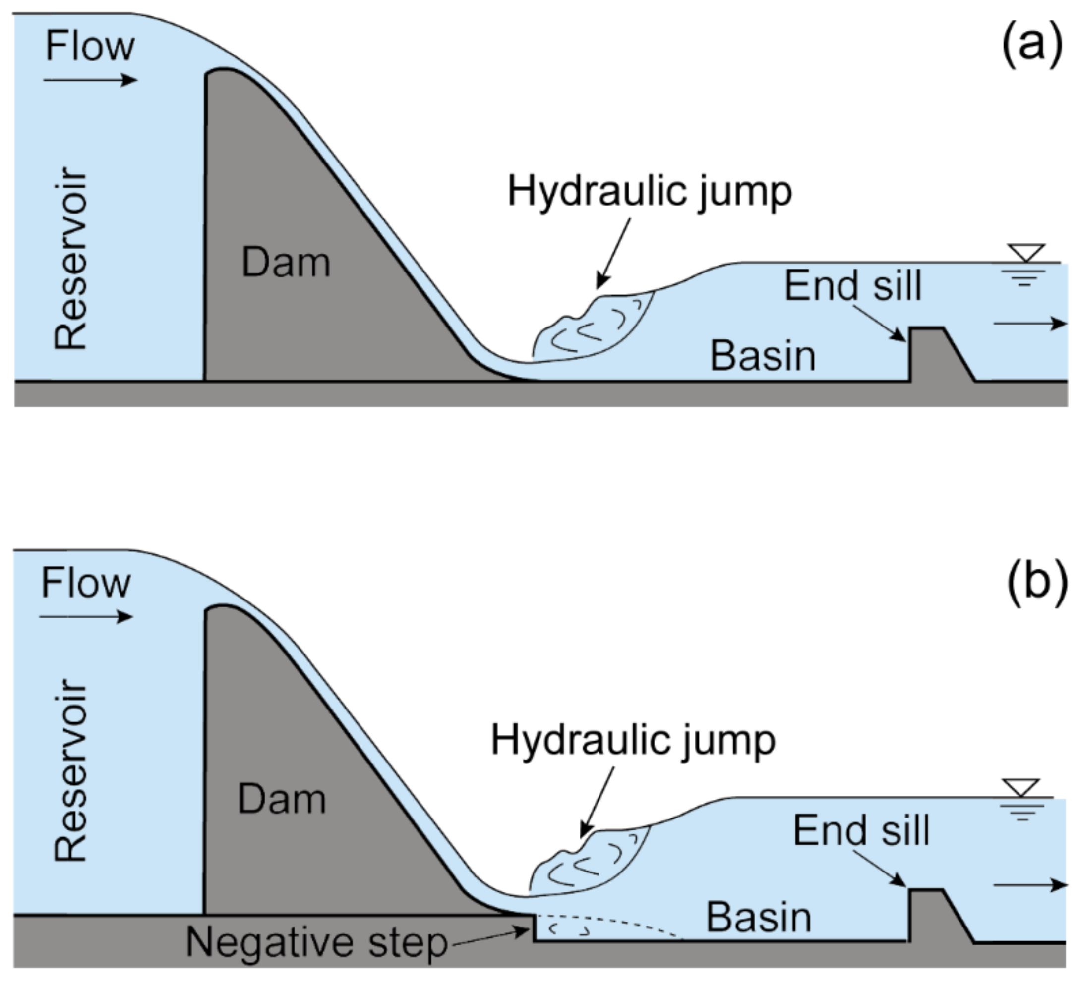
:1. Introduction
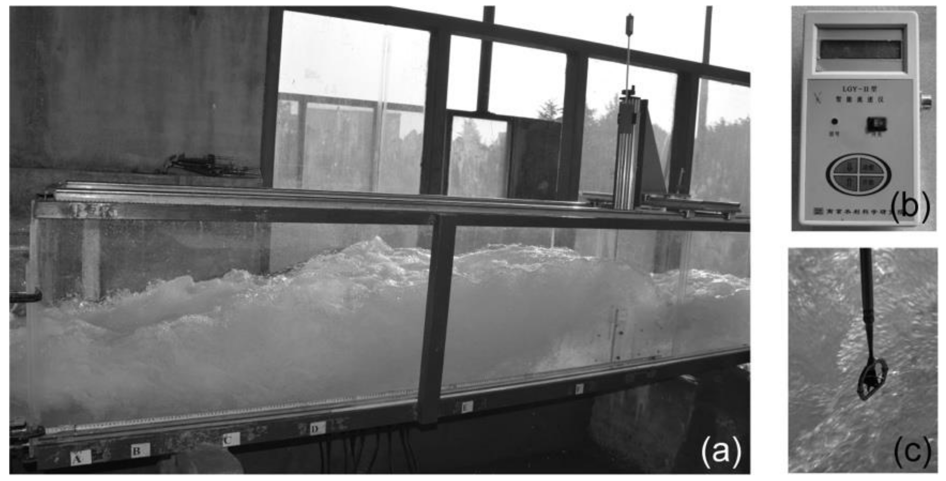
2. Experiment Setup
3. Numerical Simulations
3.1. Flow Equations
3.2. Numerical Simulation Runs and Solution Domain
3.3. Numerical Settings
3.4. Meshing and Boundary Conditions
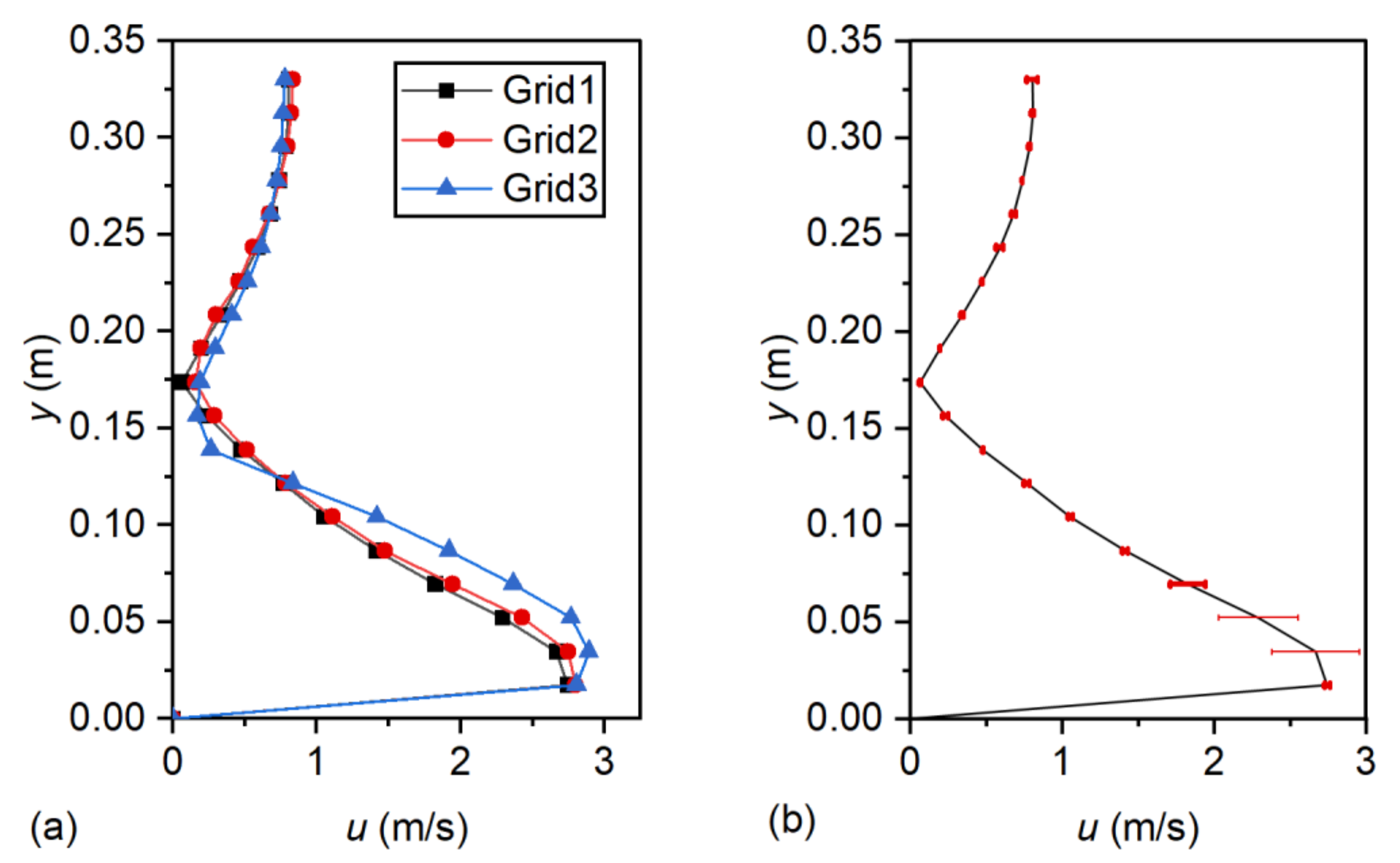
3.5. Discretization Error Analysis
4. Results
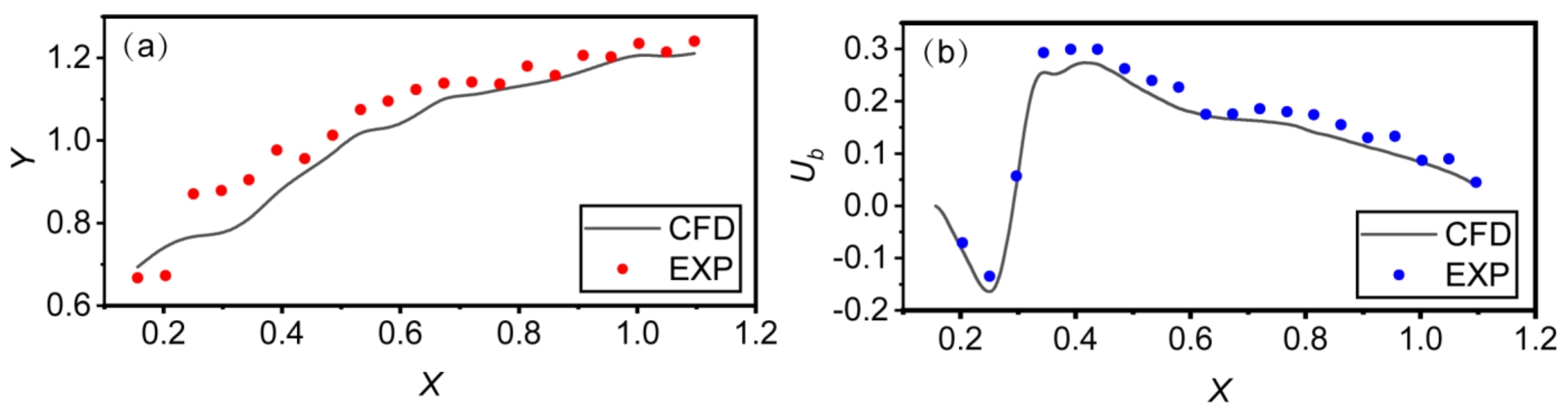
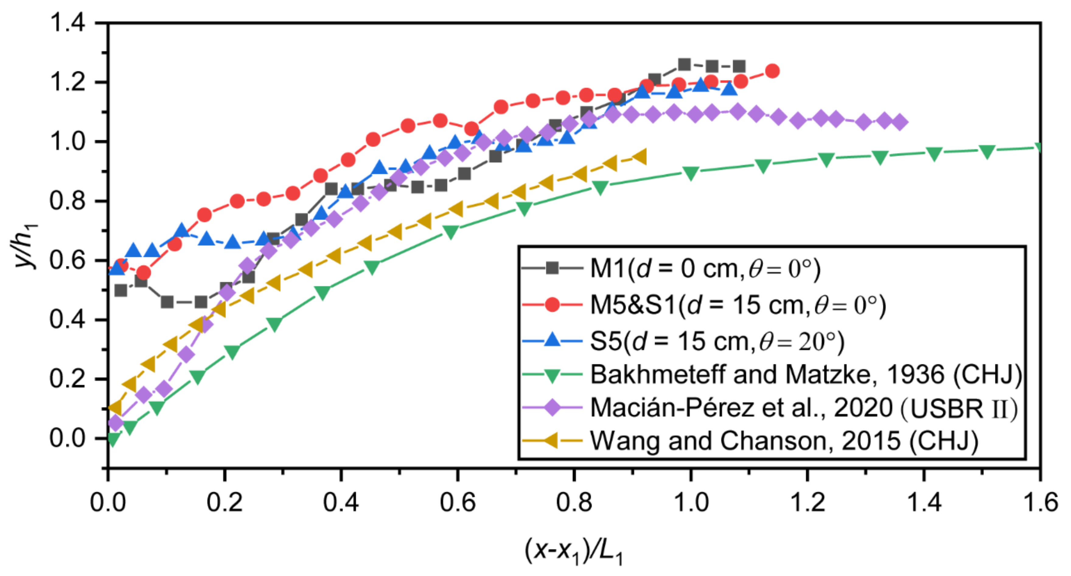
4.1. Validation of the Numerical Model
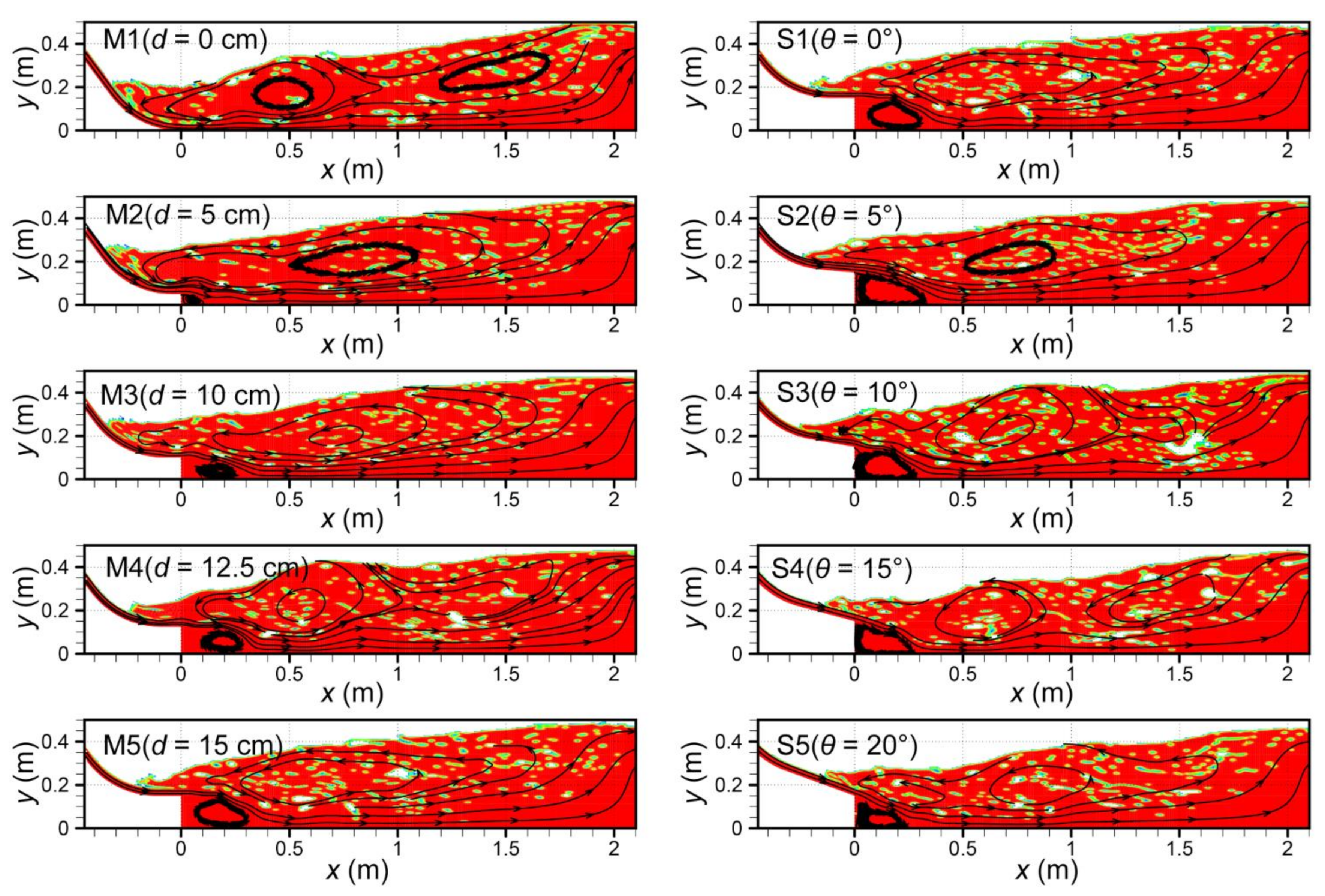
4.2. Flow Pattern
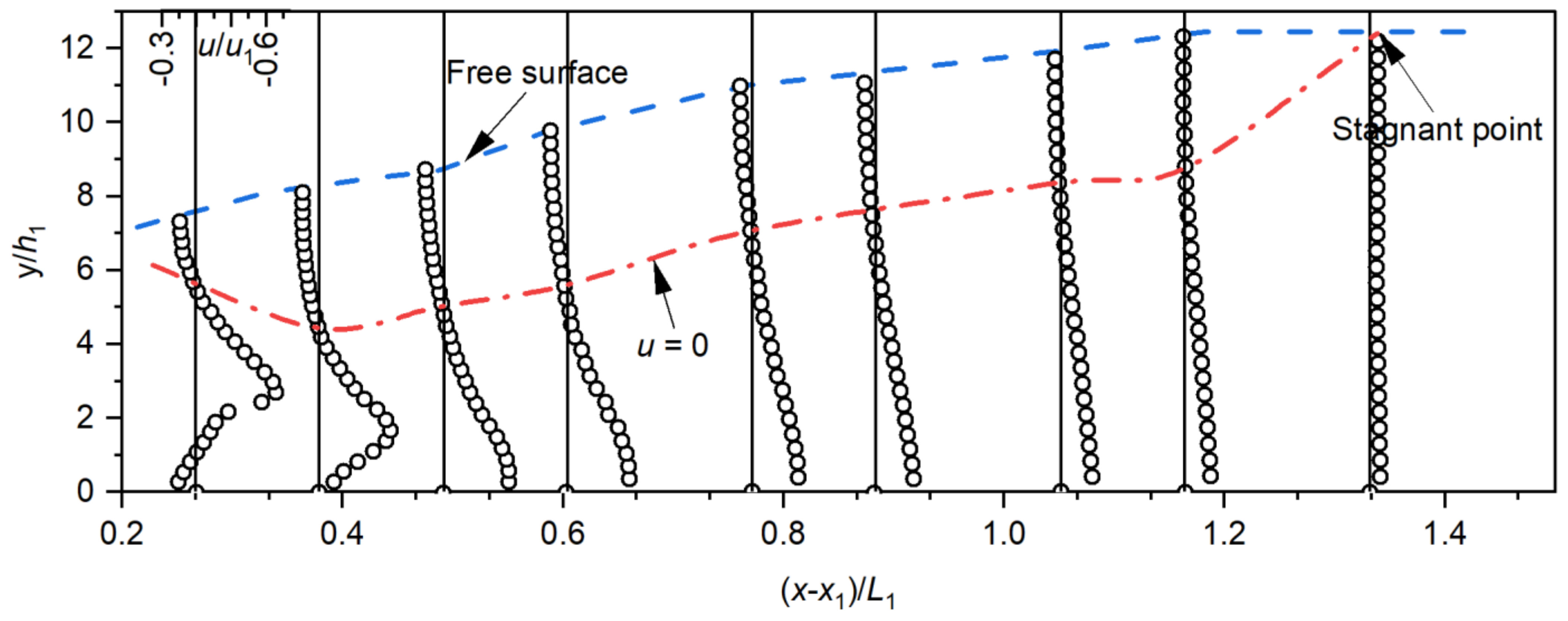
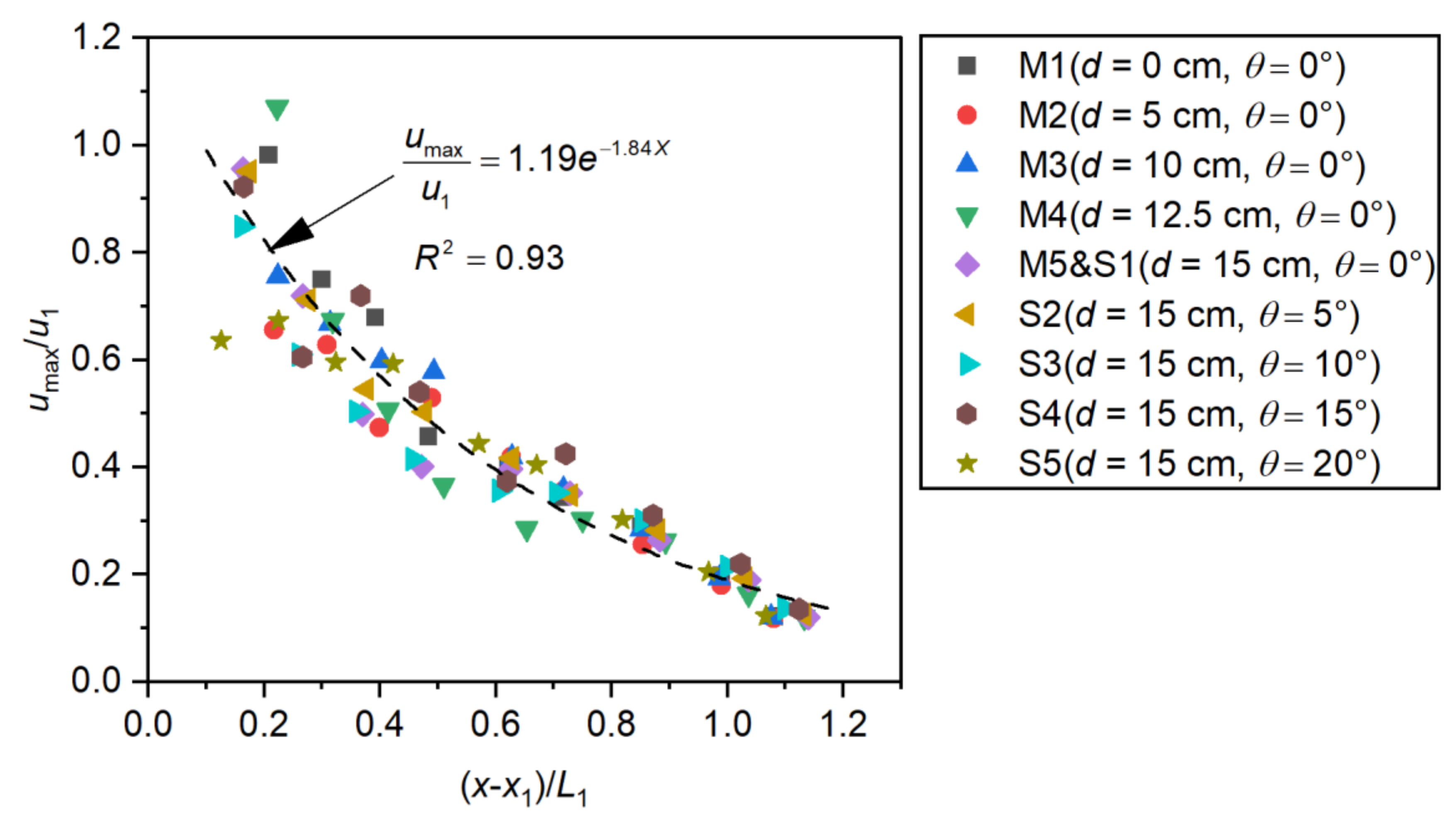
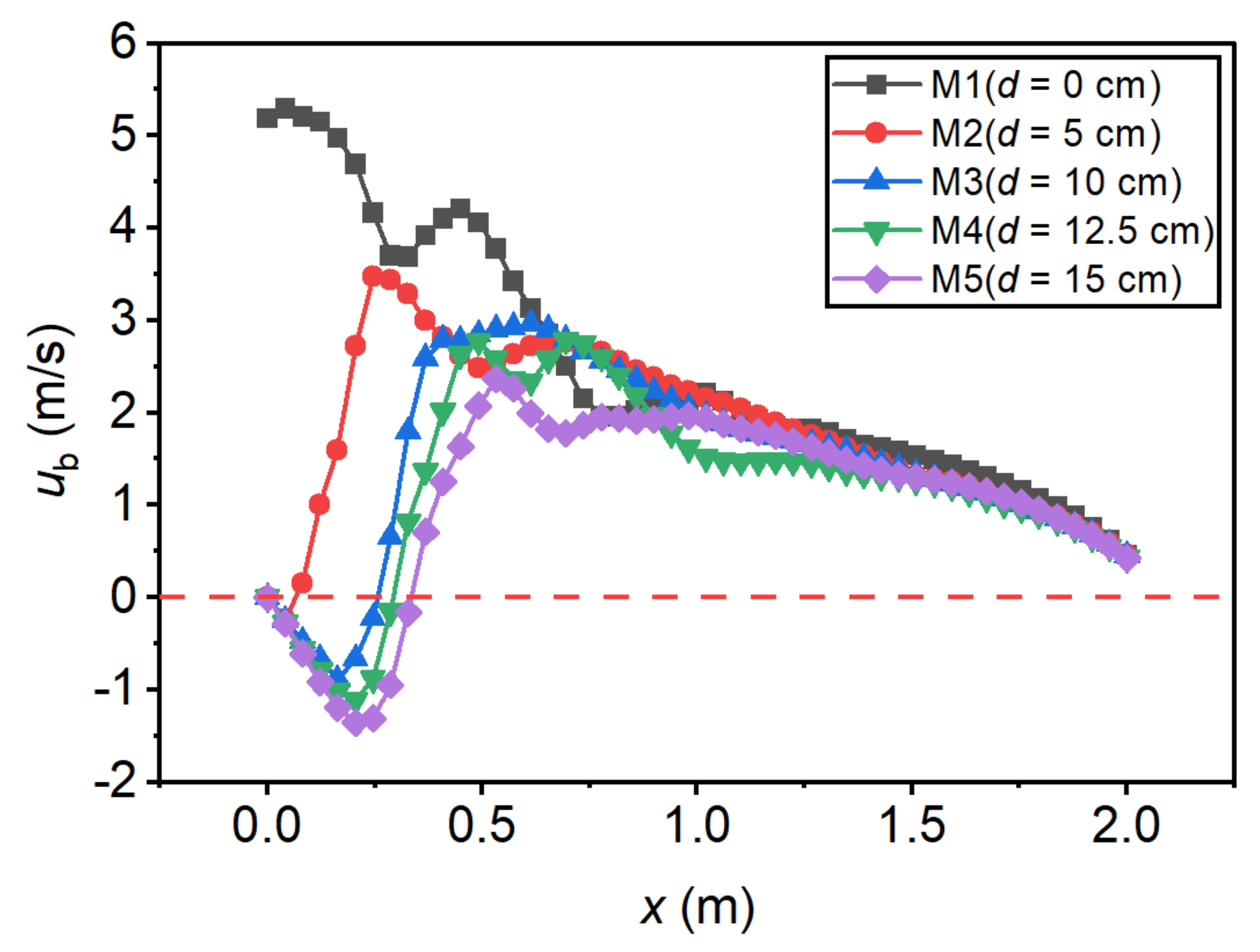
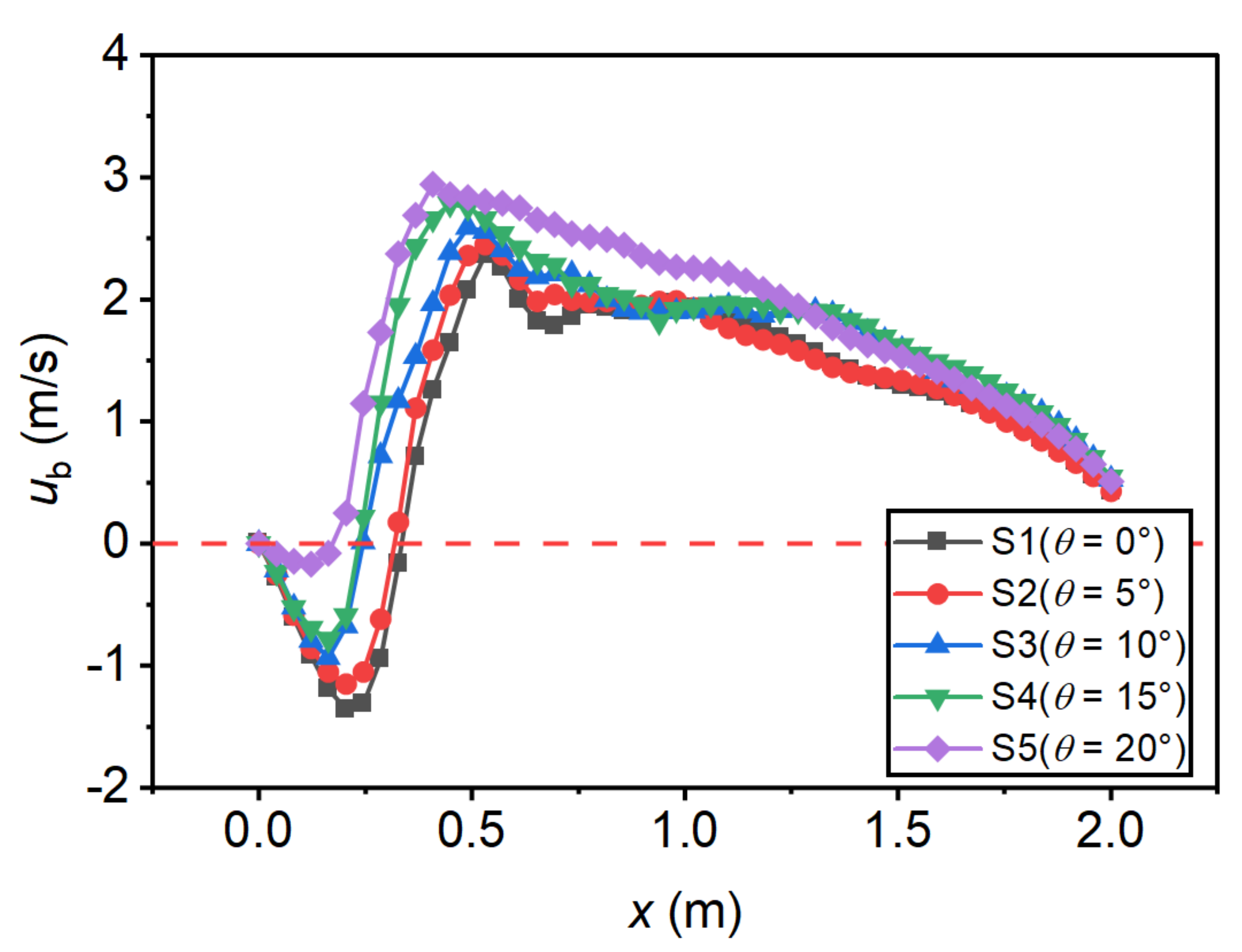
4.3. Velocity Profile
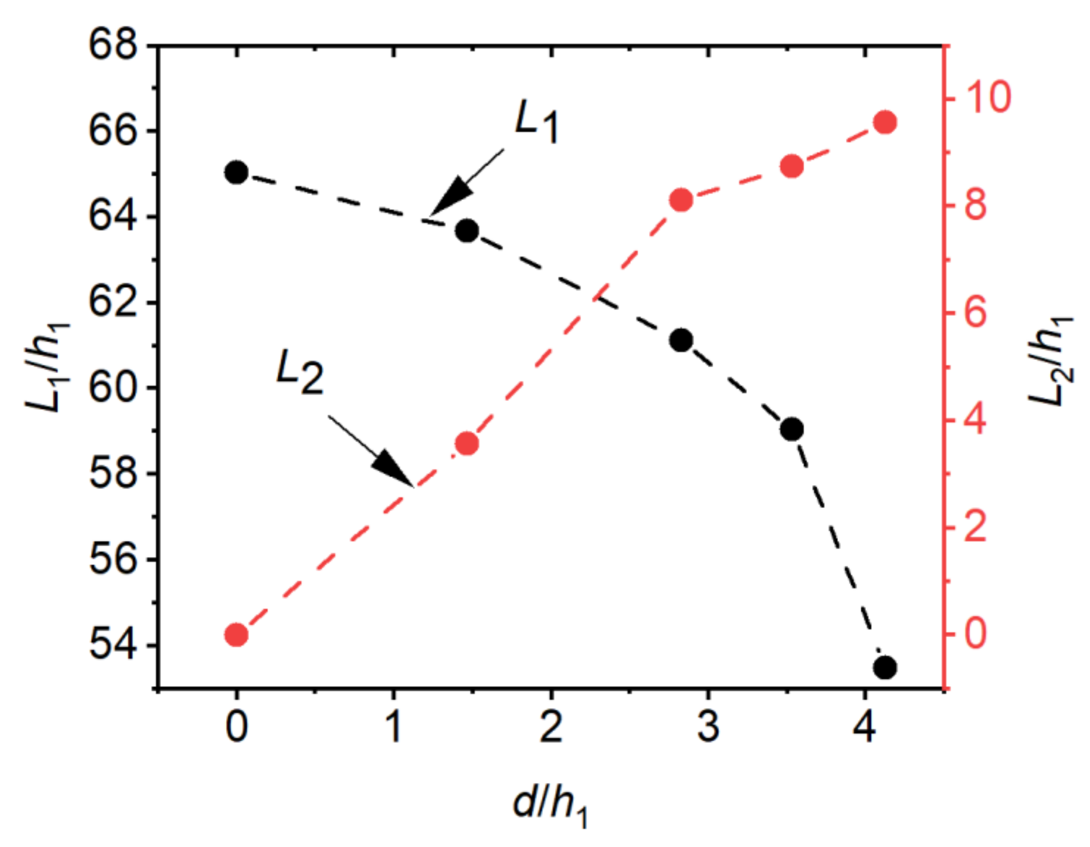
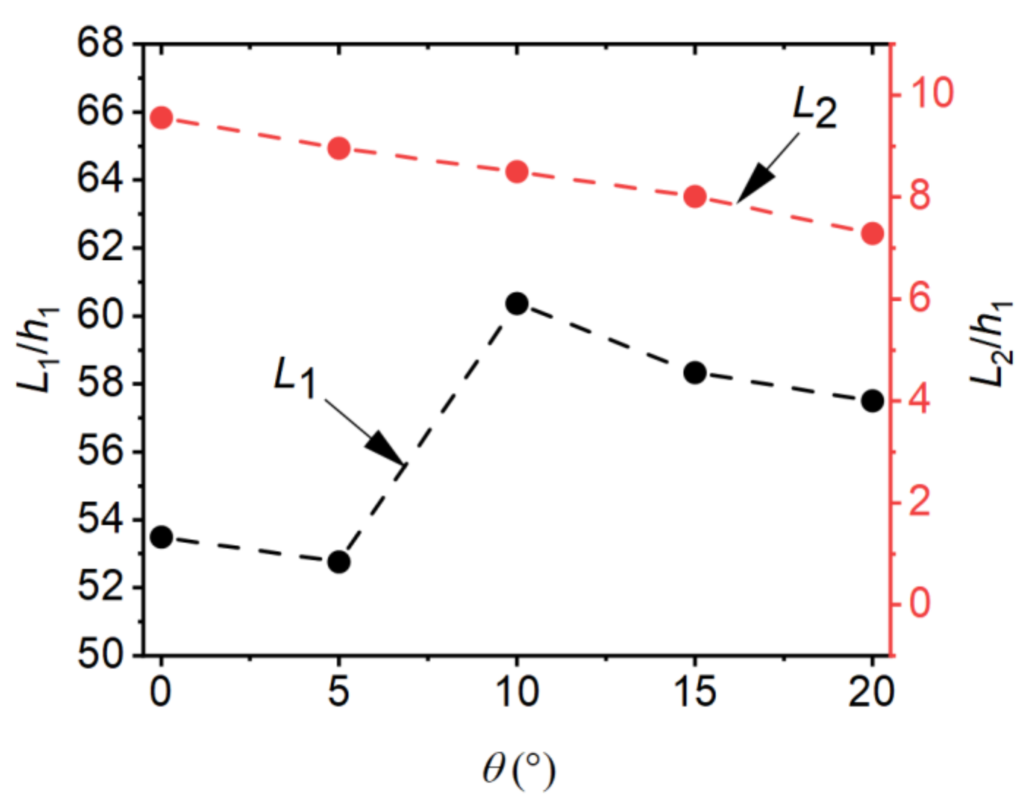
4.4. Roller Length and Reattachment Length
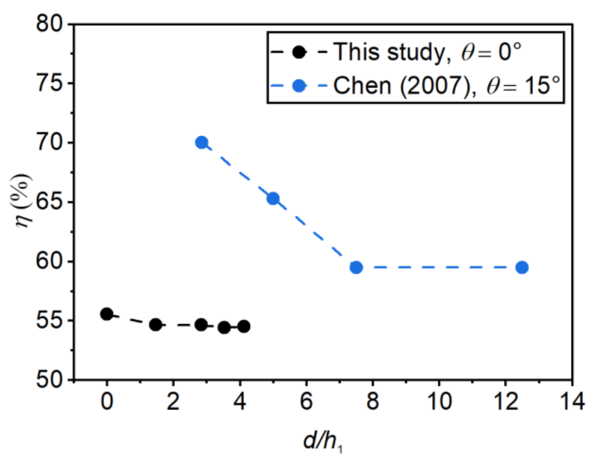
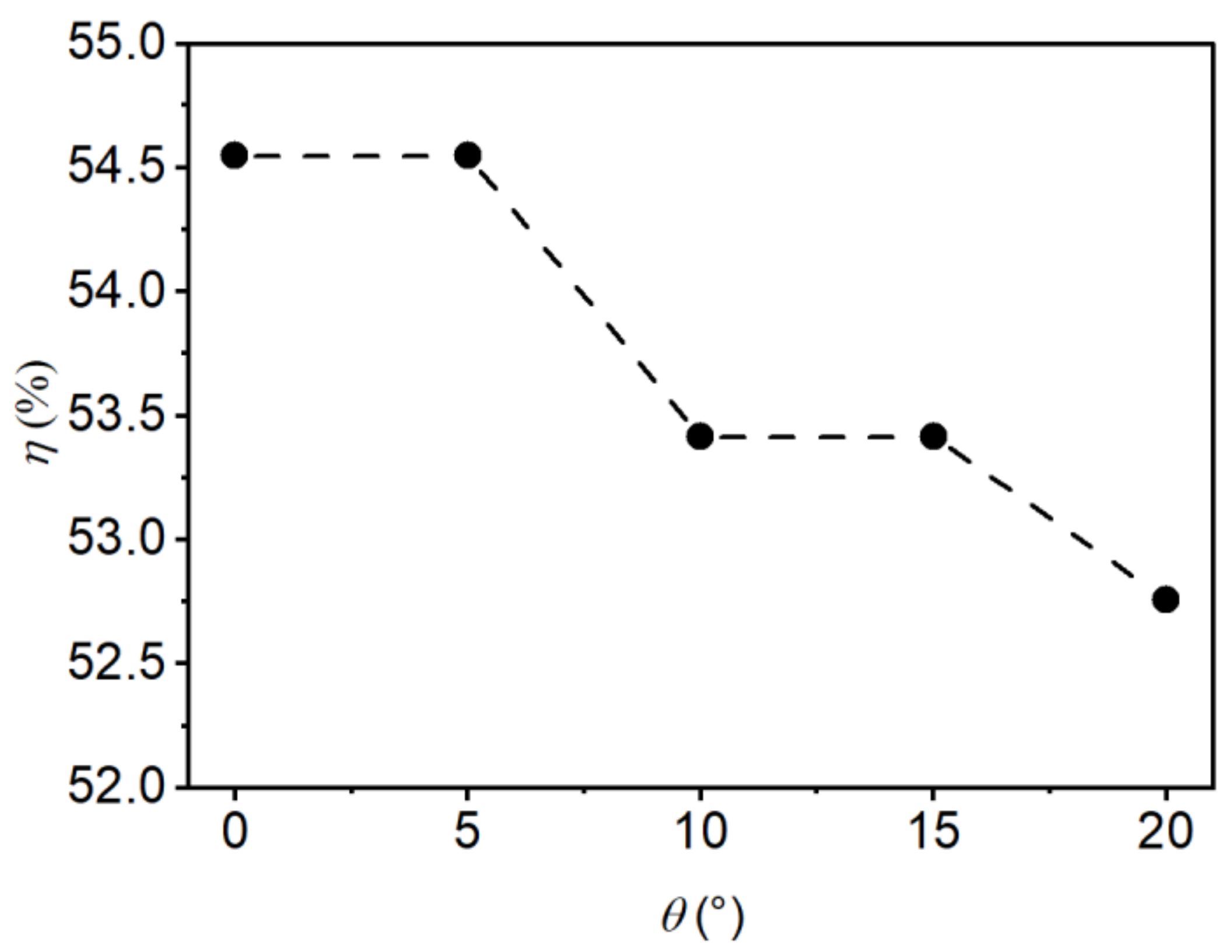
4.5. Energy Dissipation Efficiency
5. Discussion
6. Conclusions
- (1)
- The influence of step height on the flow regime is significant and the influence of incident angle on the flow regime is insignificant. Increasing the step height will lead to an increase in the flow depth in the basin, so the negative-step stilling basin needs a higher sidewall than the traditional stilling basin. However, the step height should be less than the critical height to avoid the surface jump in the basin.
- (2)
- Increasing the step height will significantly reduce the bottom flow velocity, and increasing the incident angle will significantly increase the critical bottom flow velocity. Therefore, the design of the negative-step stilling basin needs to consider the influence of the step height and the incident angle to achieve the most ideal design geometry.
- (3)
- Using a higher step height can reduce the roller length of the jump in the negative-step stilling basin, thus shortening the length of the dissipation basin. The reattachment length maintains a good linear relationship with both the step height and incident angle.
- (4)
- Within the scope of this study, changing the step height and incident angle did not have a strong effect on the total energy dissipation efficiency of the negative-step stilling basin.
Author Contributions
Funding
Data Availability Statement
Acknowledgments
Conflicts of Interest
Abbreviations
| d | Step height |
| θ | Incident angle |
| Q | Flow discharge |
| q | Unit discharge |
| h1 | Mean depth at the jump toe |
| u1 | Mean velocity at the jump toe |
| F1 | Froude number at the jump toe |
| ht | Tailwater depth |
| GCI | Grid convergence index |
| x1 | Jump toe position |
| L1 | Roller length |
| h1 | Flow depth at jump toe |
| ub | Bottom velocity |
| E | Submergence parameter |
| umax | Maximum velocity |
| L2 | Reattachment length |
| η | Energy dissipation efficiency |
| dc | Critical step height |
References
- Barjastehmaleki, S.; Fiorotto, V.; Caroni, E. Spillway Stilling Basins Lining Design via Taylor Hypothesis. J. Hydraul. Eng. 2016, 142, 04016010. [Google Scholar] [CrossRef]
- Li, S. Research on Hydrodynamic Loads of Stilling Basin with Drop Sill. Ph.D. thesis, Tianjin University, Tianjin, China, 2012. (In Chinese). [Google Scholar]
- Sun, S.; Liu, H.; Xia, Q.; Wang, X. Study on Stilling Basin with Step-down Floor for Energy Dissipation of Hydraulic Jump in High Dams. J. Hydraul. Eng. 2005, 361, 1188–1193. (In Chinese) [Google Scholar]
- Huang, G.; Diao, M.; Jiang, L.; Wang, C.; Jia, W. Experimental Study on Wave Characteristics of Stilling Basin with a Negative Step. Entropy 2022, 24, 445. [Google Scholar] [CrossRef] [PubMed]
- Hager, W.H. B-Jumps at Abrupt Channel Drops. J. Hydraul. Eng. 1985, 111, 861–866. [Google Scholar] [CrossRef]
- Hager, W.H.; Bretz, N.V. Hydraulic Jumps at Positive and Negative Steps. J. Hydraul. Res. 1986, 24, 237–253. [Google Scholar] [CrossRef]
- Ohtsu, I.; Yasuda, Y. Transition from Supercritical to Subcritical Flow at an Abrupt Drop. J. Hydraul. Res. 1991, 29, 309–328. [Google Scholar] [CrossRef]
- Mossa, M. On the Oscillating Characteristics of Hydraulic Jumps. J. Hydraul. Res. 1999, 37, 541–558. [Google Scholar] [CrossRef]
- Tokyay, N.D.; Altan-Sakarya, A.B. Local Energy Losses at Positive and Negative Steps in Subcritical Open Channel Flows. Water SA 2011, 37, 237–244. [Google Scholar] [CrossRef] [Green Version]
- Moore, W.L.; Morgan, C.W. The Hydraulic Jump at an Abrupt Drop. Trans. Am. Soc. Civ. Eng. 1959, 124, 507–516. [Google Scholar] [CrossRef]
- Eroğlu, N.; Taştan, K. Local Energy Losses for Wave-Type Flows at Abrupt Bottom Changes. J. Irrig. Drain. Eng. 2020, 146, 04020029. [Google Scholar] [CrossRef]
- Jia, W.; Diao, M.; Jiang, L.; Huang, G. Time-Frequency Characteristics of Fluctuating Pressure on the Bottom of the Stilling Basin with Step-Down Floor Based on Hilbert–Huang Transform. Math. Probl. Eng. 2021, 2021, 7246488. [Google Scholar] [CrossRef]
- Jia, W.; Diao, M.; Jiang, L.; Huang, G. Fluctuating Characteristics of the Stilling Basin with a Negative Step Based on Hilbert-Huang Transform. Water 2021, 13, 2673. [Google Scholar] [CrossRef]
- Valero, D.; Bung, D.B.; Crookston, B.M. Energy Dissipation of a Type III Basin under Design and Adverse Conditions for Stepped and Smooth Spillways. J. Hydraul. Eng. 2018, 144, 04018036. [Google Scholar] [CrossRef]
- Carvalho, R.F.; Lemos, C.M.; Ramos, C.M. Numerical Computation of the Flow in Hydraulic Jump Stilling Basins. J. Hydraul. Res. 2008, 46, 739–752. [Google Scholar] [CrossRef]
- Celik, I.B.; Ghia, U.; Roache, P.J.; Freitas, C.J. Procedure for Estimation and Reporting of Uncertainty Due to Discretization in CFD Applications. J. Fluids Eng.-Trans. ASME 2008, 130, 078001. [Google Scholar]
- Zhou, Z.; Wang, J. Numerical Modeling of 3D Flow Field among a Compound Stilling Basin. Math. Probl. Eng. 2019, 2019, 5934274. [Google Scholar] [CrossRef] [Green Version]
- Macián-Pérez, J.F.; Vallés-Morán, F.G.; García-Bartual, R. Assessment of the Performance of a Modified USBR Type II Stilling Basin by a Validated CFD Model. J. Irrig. Drain. Eng. 2021, 147, 04021052. [Google Scholar] [CrossRef]
- Kirkgoz, M.S.; Akoz, M.S.; Oner, A.A. Numerical Modeling of Flow over a Chute Spillway. J. Hydraul. Res. 2009, 47, 790–797. [Google Scholar] [CrossRef]
- Akoz, M.S.; Gumus, V.; Kirkgoz, M.S. Numerical Simulation of Flow over a Semicylinder Weir. J. Irrig. Drain. Eng. 2014, 140, 04014016. [Google Scholar] [CrossRef]
- Macián-Pérez, J.F.; Bayón, A.; García-Bartual, R.; Amparo, L.-J.P.; Vallés-Morán, F.J. Characterization of Structural Properties in High Reynolds Hydraulic Jump Based on CFD and Physical Modeling Approaches. J. Hydraul. Eng. 2020, 146, 04020079. [Google Scholar] [CrossRef]
- Bombardelli, F.A.; Meireles, I.; Matos, J. Laboratory Measurements and Multi-Block Numerical Simulations of the Mean Flow and Turbulence in the Non-Aerated Skimming Flow Region of Steep Stepped Spillways. Environ. Fluid Mech. 2011, 11, 263–288. [Google Scholar] [CrossRef] [Green Version]
- Launder, B.E.; Spalding, D.B. The Numerical Computation of Turbulent Flows. Comput. Methods Appl. Mech. Eng. 1974, 3, 269–289. [Google Scholar] [CrossRef]
- Yakhot, V.; Orszag, S.A. Renormalization-Group Analysis of Turbulence. Phys. Rev. Lett. 1986, 57, 1722–1724. [Google Scholar] [CrossRef] [PubMed] [Green Version]
- Hirt, C.W.; Nichols, B.D. Volume of Fluid (VOF) Method for the Dynamics of Free Boundaries. J. Comput. Phys. 1981, 39, 201–225. [Google Scholar] [CrossRef]
- Helal, E.; Abdelhaleem, F.S.; Elshenawy, W.A. Numerical Assessment of the Performance of Bed Water Jets in Submerged Hydraulic Jumps. J. Irrig. Drain. Eng. 2020, 146, 04020014. [Google Scholar] [CrossRef]
- Issa, R.I. Solution of the Implicitly Discretised Fluid Flow Equations by Operator-Splitting. J. Comput. Phys. 1986, 62, 40–65. [Google Scholar] [CrossRef]
- Maranzoni, A.; Tomirotti, M. 3D CFD Analysis of the Performance of Oblique and Composite Side Weirs in Converging Channels. J. Hydraul. Res. 2021, 59, 586–604. [Google Scholar] [CrossRef]
- Salehi, S.; Mostaani, A.; Azimi, A.H. Experimental and Numerical Investigations of Flow over and under Weir-Culverts with a Downstream Ramp. J. Irrig. Drain. Eng. 2021, 147, 04021029. [Google Scholar] [CrossRef]
- Kawagoshi, N.; Hager, W.H. B-Jump in Sloping Channel, II. J. Hydraul. Res. 1990, 28, 461–480. [Google Scholar] [CrossRef]
- Hager, W.H. B-Jump in Sloping Channel. J. Hydraul. Res. 1988, 26, 539–558. [Google Scholar] [CrossRef]
- Bakhmeteff, B.A.; Matzke, A.E. The Hydraulic Jump in Terms of Dynamic Similarity. Trans. Am. Soc. Civ. Eng. 1936, 101, 630–647. [Google Scholar] [CrossRef]
- Wang, H.; Chanson, H. Experimental Study of Turbulent Fluctuations in Hydraulic Jumps. J. Hydraul. Eng. 2015, 141, 04015010. [Google Scholar] [CrossRef]
- Macián-Pérez, J.F.; Vallés-Morán, F.J.; Sánchez-Gómez, S.; De-Rossi-Estrada, M.; García-Bartual, R. Experimental Characterization of the Hydraulic Jump Profile and Velocity Distribution in a Stilling Basin Physical Model. Water 2020, 12, 1758. [Google Scholar] [CrossRef]
- Nyantekyi-Kwakye, B.; Clark, S.P.; Tachie, M.F.; Malenchak, J.; Muluye, G. Flow Characteristics within the Recirculation Region of Three-Dimensional Turbulent Offset Jet. J. Hydraul. Res. 2015, 53, 230–242. [Google Scholar] [CrossRef]
- Padulano, R.; Fecarotta, O.; Del Giudice, G.; Carravetta, A. Hydraulic Design of a USBR Type II Stilling Basin. J. Irrig. Drain. Eng. 2017, 143, 04017001. [Google Scholar] [CrossRef] [Green Version]
- Chen, H. Experimental Study on the Hydraulic Characteristics of Hydraulic Jump Stilling Basin with a Drop Step. Master’s Thesis, Kunming University of Technology, Kunming, China, 2007. (In Chinese). [Google Scholar]
- Wang, Y.; Politano, M.; Weber, L. Spillway Jet Regime and Total Dissolved Gas Prediction with a Multiphase Flow Model. J. Hydraul. Res. 2019, 57, 26–38. [Google Scholar] [CrossRef]
- Zheng, X. Hydraulic Design Study of the Step-Down Bottom Energy Dissipator. Master’s Thesis, Kunming University of Technology, Kunming, China, 2010. (In Chinese). [Google Scholar]
- Armenio, V.; Toscano, P.; Fiorotto, V. On the Effects of a Negative Step in Pressure Fluctuations at the Bottom of a Hydraulic Jump. J. Hydraul. Res. 2000, 38, 359–368. [Google Scholar] [CrossRef]
- Bai, R.; Wang, H.; Tang, R.; Liu, S.; Xu, W. Roller Characteristics of Preaerated High-Froude-Number Hydraulic Jumps. J. Hydraul. Eng. 2021, 147, 04021008. [Google Scholar] [CrossRef]


| No. | Name | Dam Height (m) | Design Discharge (m3/s) | Step Height (m) |
|---|---|---|---|---|
| 1 | Xiangjiaba | 162.0 | 41,200 | 9.0 |
| 2 | Huangjinping | 95.5 | 5650 | - |
| 3 | Jin’anqiao | 160.0 | 11,668 | - |
| 4 | Guanyinyuan | 159.0 | 16,900 | 7.5 |
| 5 | Liyuan | 155.0 | 11,361 | 15.8 |
| 6 | Guandi | 168.0 | 14,000 | 6.5 |
| 7 | Tingzikou | 110.0 | 34,500 | 8.0 |
| Run | d (cm) | θ (°) | Q (m3/s) | q (m2/s) | h1 (m) | u1 (m/s) | F1 | ht (m) |
|---|---|---|---|---|---|---|---|---|
| M1 | 0 | 0 | 0.09 | 0.18 | 0.033 | 5.386 | 9.4 | 0.388 |
| M2 | 5 | 0 | 0.09 | 0.18 | 0.034 | 5.262 | 9.1 | 0.388 |
| M3 | 10 | 0 | 0.09 | 0.18 | 0.037 | 5.091 | 8.6 | 0.388 |
| M4 | 12.5 | 0 | 0.09 | 0.18 | 0.035 | 5.087 | 8.6 | 0.388 |
| M5 (S1) | 15 | 0 | 0.09 | 0.18 | 0.036 | 4.945 | 8.3 | 0.388 |
| S2 | 15 | 5 | 0.09 | 0.18 | 0.038 | 4.782 | 7.9 | 0.388 |
| S3 | 15 | 10 | 0.09 | 0.18 | 0.034 | 5.367 | 9.4 | 0.388 |
| S4 | 15 | 15 | 0.09 | 0.18 | 0.034 | 5.301 | 9.2 | 0.388 |
| S5 | 15 | 20 | 0.09 | 0.18 | 0.035 | 5.126 | 8.7 | 0.388 |
| y (m) | P | ||||||||
|---|---|---|---|---|---|---|---|---|---|
| 0.017 | 2.742 | 2.799 | 2.804 | 0.021 | 0.002 | 1.3 | 1.3 | 9.45 | 0.7 |
| 0.035 | 2.667 | 2.744 | 2.890 | 0.029 | 0.053 | 1.3 | 1.3 | 2.42 | 10.8 |
| 0.052 | 2.292 | 2.427 | 2.764 | 0.059 | 0.139 | 1.3 | 1.3 | 3.48 | 11.3 |
| 0.069 | 1.824 | 1.947 | 2.367 | 0.067 | 0.215 | 1.3 | 1.3 | 4.69 | 6.3 |
| 0.087 | 1.415 | 1.476 | 1.919 | 0.043 | 0.300 | 1.3 | 1.3 | 7.59 | 1.2 |
| 0.104 | 1.054 | 1.108 | 1.416 | 0.051 | 0.277 | 1.3 | 1.3 | 6.62 | 1.5 |
| 0.122 | 0.767 | 0.788 | 0.835 | 0.027 | 0.059 | 1.3 | 1.3 | 3.14 | 2.0 |
| 0.139 | 0.477 | 0.513 | 0.266 | 0.075 | 0.481 | 1.3 | 1.3 | 7.36 | 0.8 |
| 0.156 | 0.233 | 0.291 | 0.170 | 0.248 | 0.416 | 1.3 | 1.3 | 2.82 | 6.6 |
| 0.174 | 0.067 | 0.156 | 0.190 | 1.337 | 0.219 | 1.3 | 1.3 | 3.66 | 6.9 |
| 0.191 | 0.196 | 0.193 | 0.294 | 0.015 | 0.525 | 1.3 | 1.3 | 13.51 | 0.0 |
| 0.208 | 0.341 | 0.301 | 0.411 | 0.115 | 0.363 | 1.3 | 1.3 | 3.91 | 2.7 |
| 0.226 | 0.472 | 0.459 | 0.521 | 0.027 | 0.136 | 1.3 | 1.3 | 6.05 | 0.4 |
| 0.243 | 0.590 | 0.561 | 0.613 | 0.048 | 0.092 | 1.3 | 1.3 | 2.30 | 4.3 |
| 0.261 | 0.681 | 0.674 | 0.679 | 0.011 | 0.008 | 1.3 | 1.3 | 1.34 | 2.2 |
| 0.278 | 0.739 | 0.739 | 0.723 | 0.000 | 0.022 | 1.3 | 1.3 | 24.00 | 0.0 |
| 0.295 | 0.785 | 0.796 | 0.752 | 0.014 | 0.055 | 1.3 | 1.3 | 5.35 | 0.4 |
| 0.313 | 0.807 | 0.824 | 0.769 | 0.022 | 0.067 | 1.3 | 1.3 | 4.43 | 1.0 |
| 0.330 | 0.804 | 0.834 | 0.779 | 0.038 | 0.067 | 1.3 | 1.3 | 2.33 | 4.5 |
| Run | d (cm) | θ (°) | E | ||
|---|---|---|---|---|---|
| M1 | 0 | 0 | −0.380 | 0.196 | 0.41 |
| M2 | 5 | 0 | −0.383 | 0.241 | 0.29 |
| M3 | 10 | 0 | −0.377 | 0.235 | 0.30 |
| M4 | 12.5 | 0 | −0.365 | 0.229 | 0.32 |
| M5 (S1) | 15 | 0 | −0.219 | 0.164 | 0.51 |
| S2 | 15 | 5 | −0.248 | 0.182 | 0.46 |
| S3 | 15 | 10 | −0.227 | 0.191 | 0.43 |
| S4 | 15 | 15 | −0.149 | 0.191 | 0.43 |
| S5 | 15 | 20 | −0.153 | 0.206 | 0.39 |
| Run | ||||
|---|---|---|---|---|
| M1 | - | - | 0.041 | 5.293 |
| M2 | 0.041 | −0.239 | 0.245 | 3.473 |
| M3 | 0.163 | −0.892 | 0.612 | 2.954 |
| M4 | 0.204 | −1.110 | 0.694 | 2.784 |
| M5 | 0.204 | −1.356 | 0.531 | 2.365 |
| S2 | 0.204 | −1.148 | 0.531 | 2.448 |
| S3 | 0.163 | −0.932 | 0.490 | 2.588 |
| S4 | 0.163 | −0.781 | 0.449 | 2.785 |
| S5 | 0.122 | −0.169 | 0.408 | 2.944 |
Publisher’s Note: MDPI stays neutral with regard to jurisdictional claims in published maps and institutional affiliations. |
© 2022 by the authors. Licensee MDPI, Basel, Switzerland. This article is an open access article distributed under the terms and conditions of the Creative Commons Attribution (CC BY) license (https://creativecommons.org/licenses/by/4.0/).
Share and Cite
Jiang, L.; Diao, M.; Wang, C. Investigation of a Negative Step Effect on Stilling Basin by Using CFD. Entropy 2022, 24, 1523. https://doi.org/10.3390/e24111523
Jiang L, Diao M, Wang C. Investigation of a Negative Step Effect on Stilling Basin by Using CFD. Entropy. 2022; 24(11):1523. https://doi.org/10.3390/e24111523
Chicago/Turabian StyleJiang, Lei, Minjun Diao, and Chuan’ai Wang. 2022. "Investigation of a Negative Step Effect on Stilling Basin by Using CFD" Entropy 24, no. 11: 1523. https://doi.org/10.3390/e24111523