
Four-Objective Optimizations of a Single Resonance Energy Selective Electron Refrigerator


Abstract
:1. Introduction
2. Model Description and Performance Indicators
3. Multi-Objective Optimizations
4. Conclusions
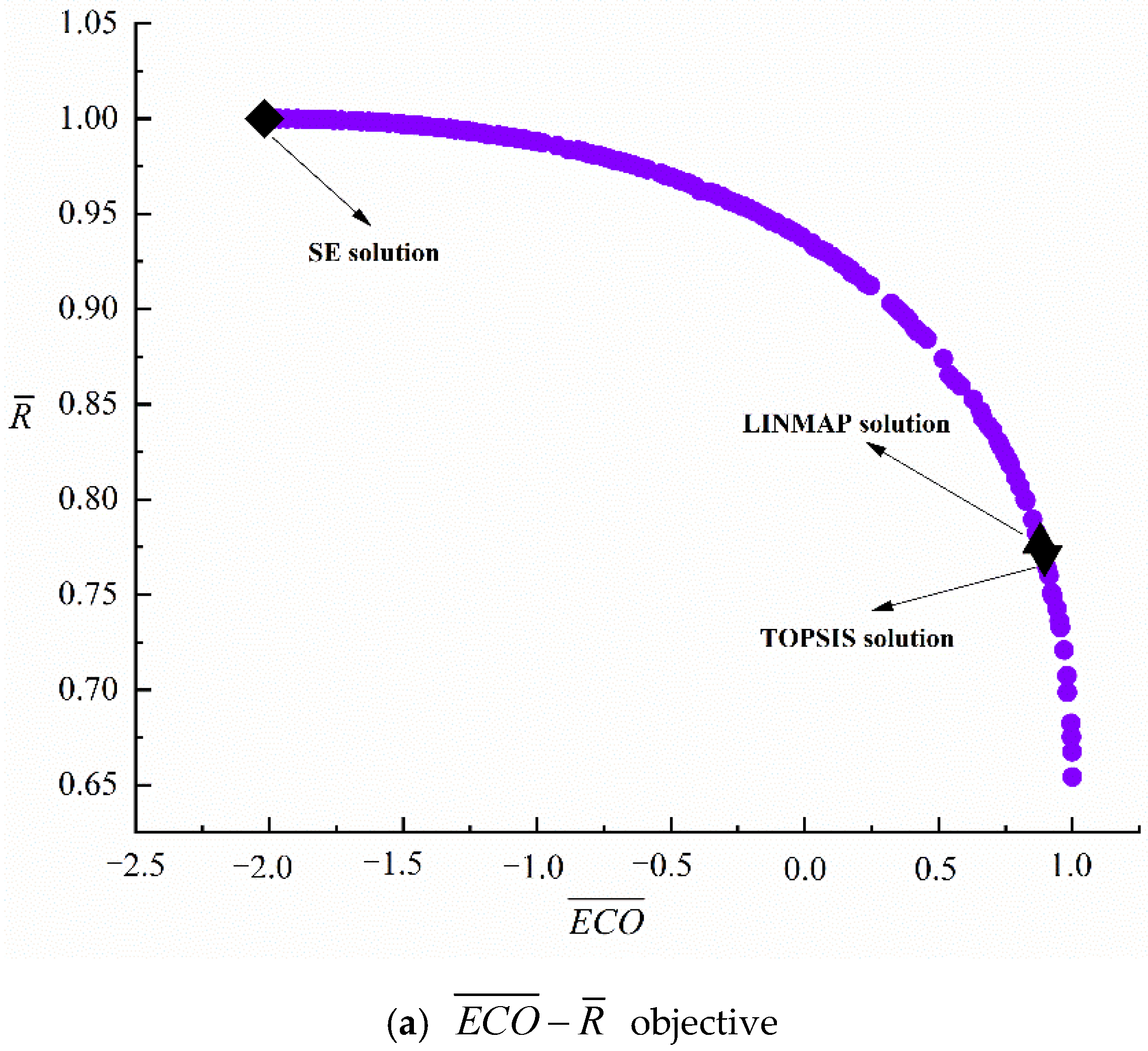
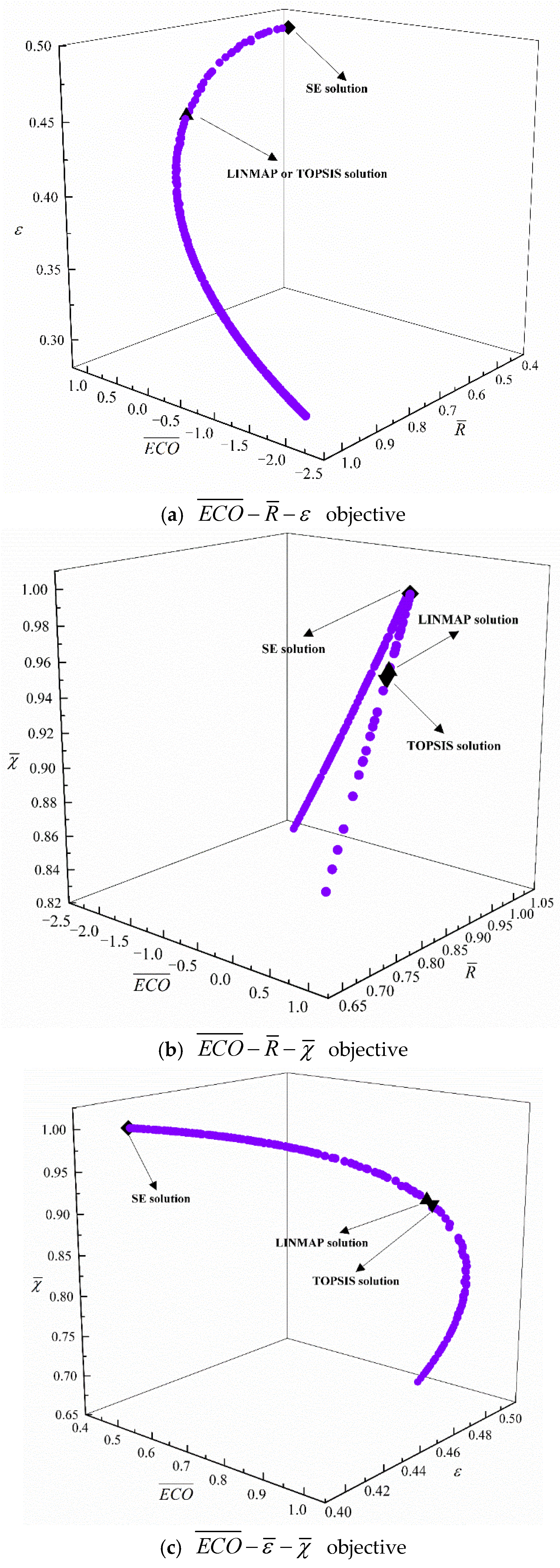
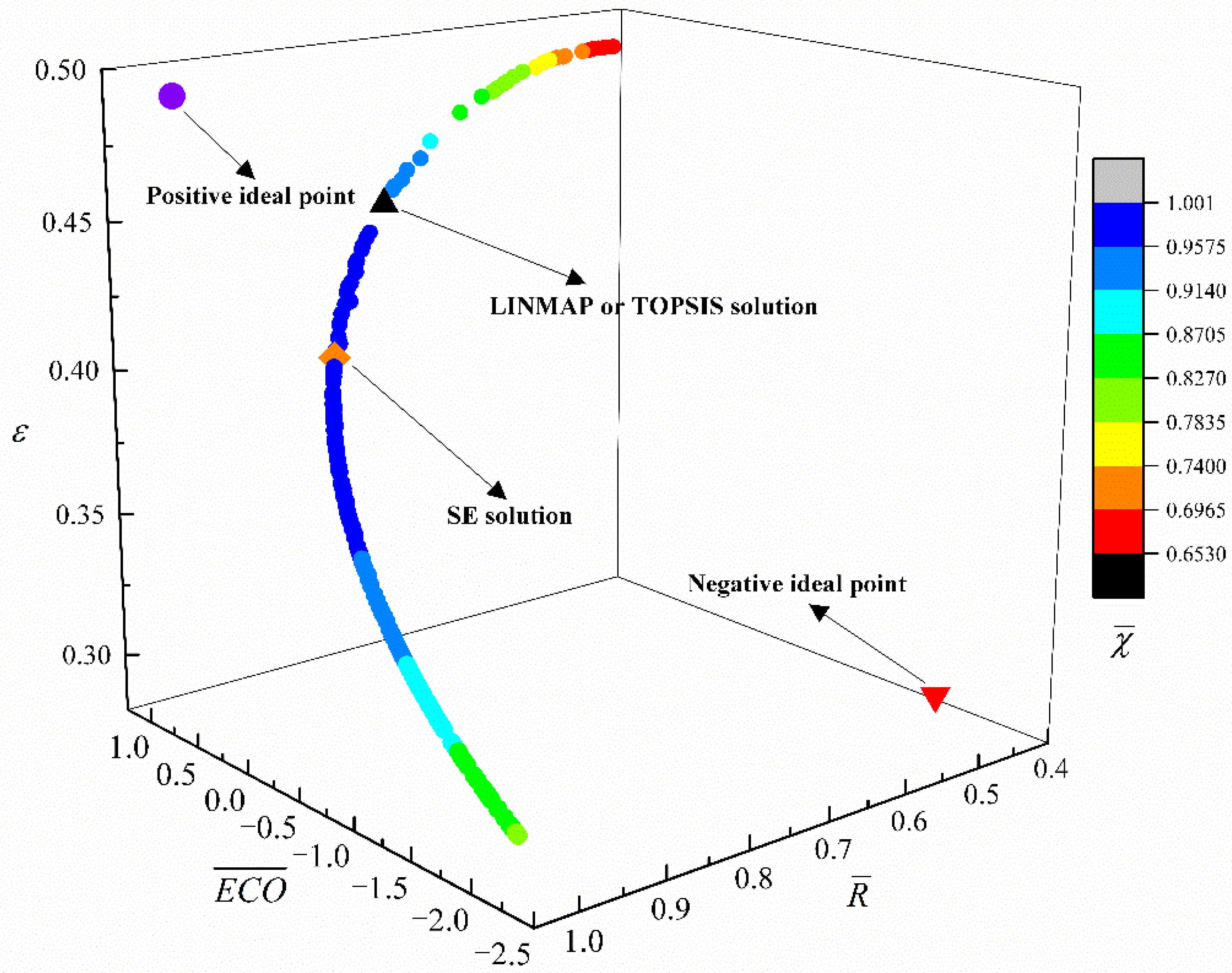
- The s obtained with LINMAP and TOPSIS approaches are 0.0812 for the MOO of , which are more reasonable than those obtained with the SE approach; at this time, the values of and are 12.5958 and 1.8267, respectively. Comparing with the s (0.1085, 0.8455, 0.1865, and 0.1780) for the four single-objective optimizations with maximum , , , and , the s of the MOO are smaller. Therefore, compared with single-objective optimization, MOO can better take different optimization objectives into account by choosing appropriate decision-making methods.
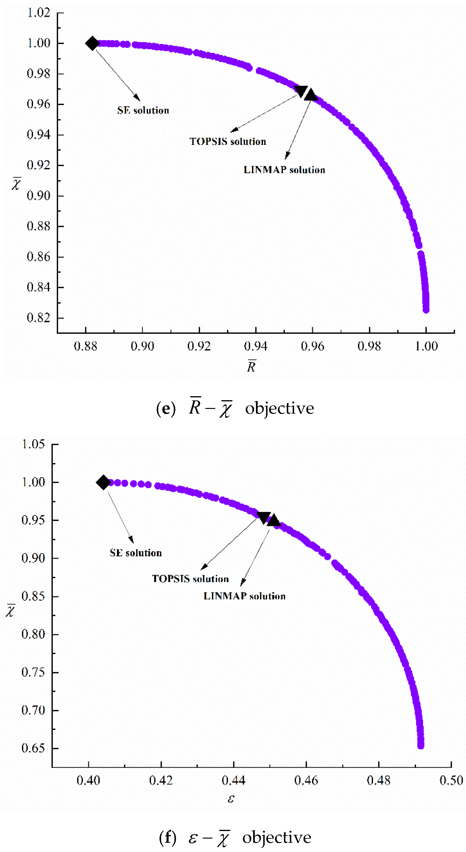
- When MOO is performed on , the is the 0.0809 obtained with the TOPSIS approach, which is the closest point to the positive ideal point and the most reasonable solution; and the corresponding values of the and are 12.5887 and 1.8050, respectively. When MOO is performed on other optimization objective combinations, the better solutions are obtained by choosing the appropriate decision-making approaches according to the design requirements.
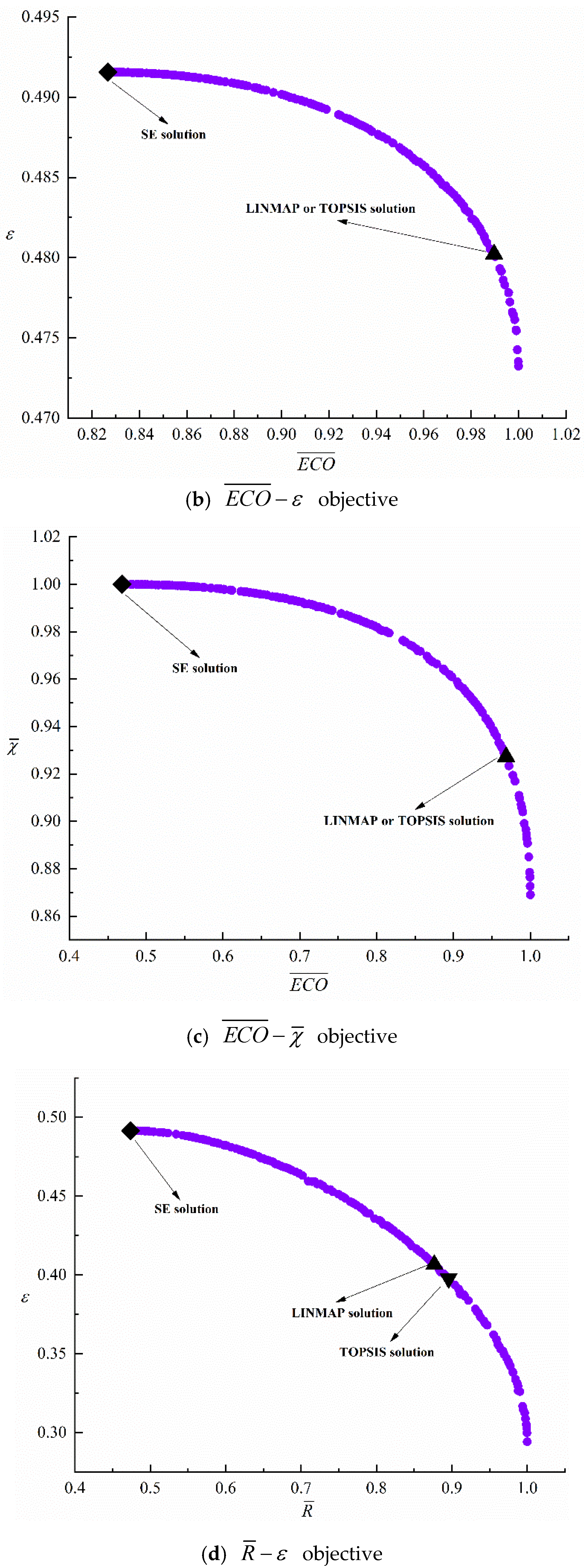
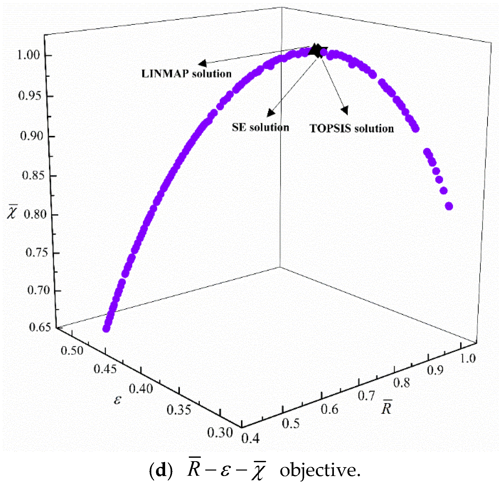
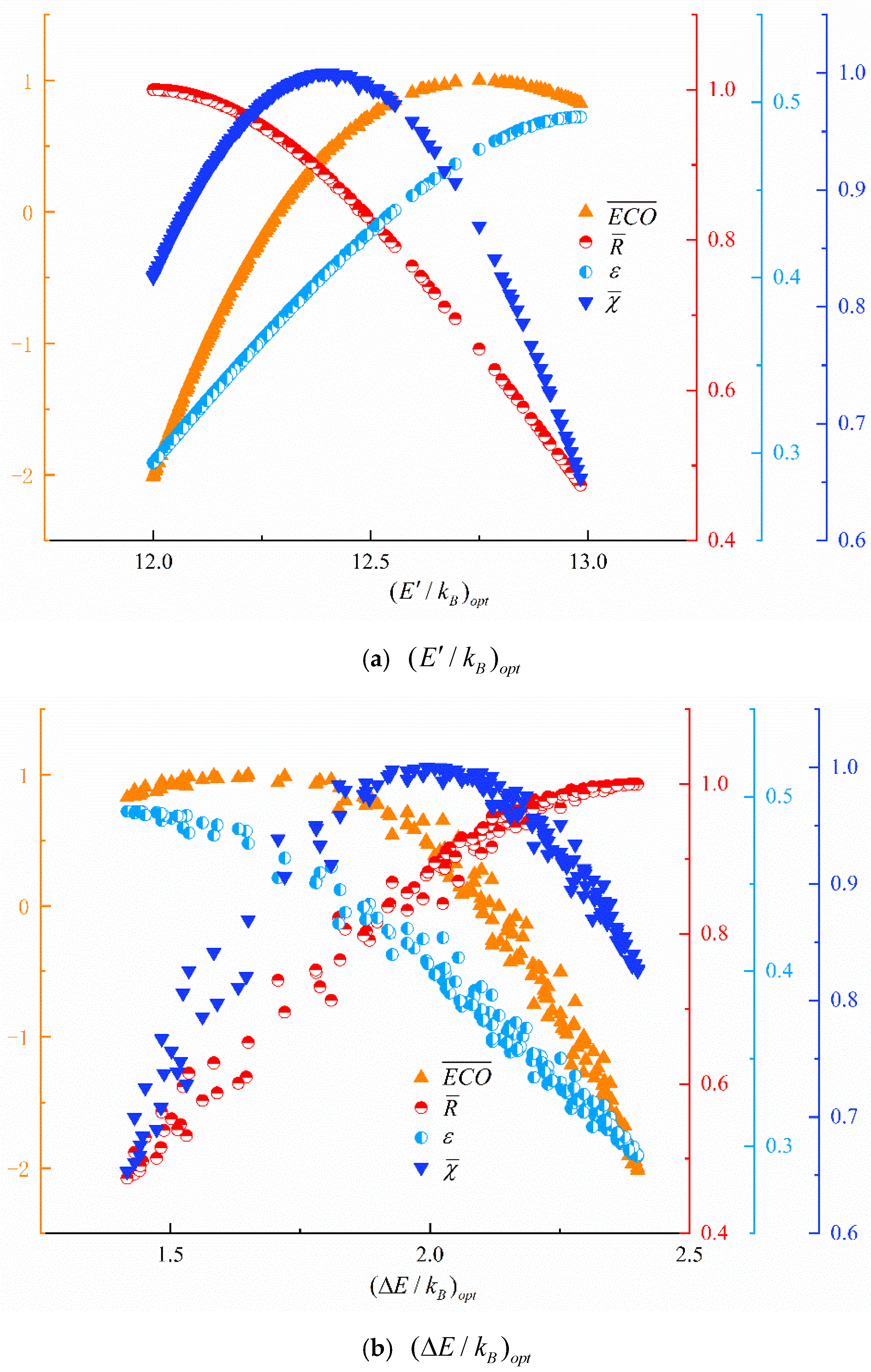
- For the MOO of , the value of ranges mainly from 12 to 13; as grows, continues to decline, continues to grow, and grow first and then decline. The value of ranges mainly from 1.5 to 2.5; as grows, continues to grow, continues to decline, and grow first and then decline. It indicates that the values of and are closely related to values of the four optimization objectives (, , , and ), and the selection of the parameters of the energy filter is very important to improve the performance of energy selective electron refrigerators.
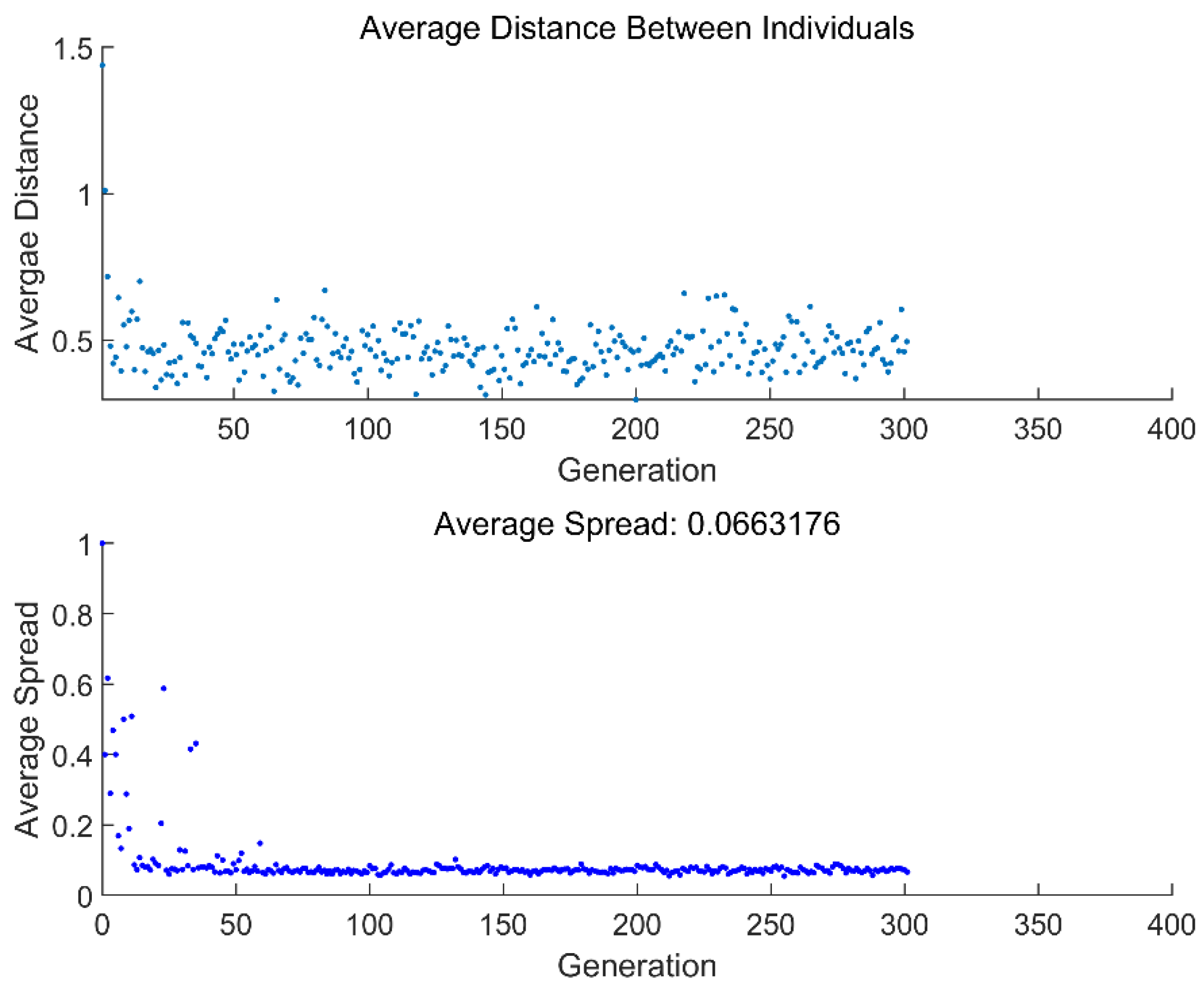
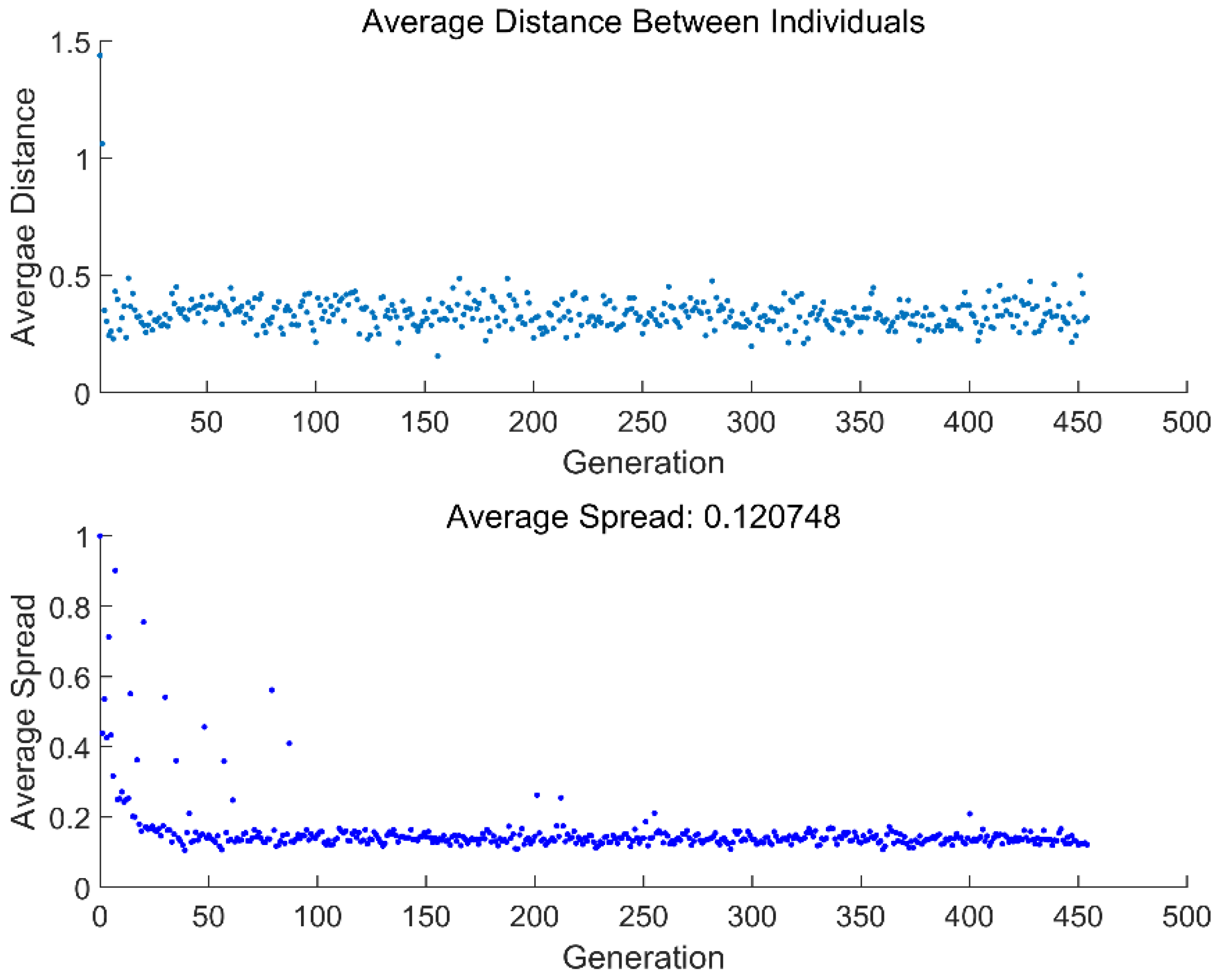
- For the MOO of and , the average distances range mainly from 0 to 0.5 and change slightly; the average spreads range mainly from 0 to 0.2, vary significantly before the 100th generations, and then remain stable.
- NSGA-II and FTT theory are effective tools to guide the designs of energy selective electron refrigerators.
Author Contributions
Funding
Institutional Review Board Statement
Informed Consent Statement
Acknowledgments
Conflicts of Interest
Nomenclature
| Exergy output rate () | |
| Energy boundary () | |
| Ecological function | |
| Bias voltage | |
| Fermi distributions of electrons | |
| A defined function | |
| Plank constant () | |
| Boltzmann constant () | |
| Heat leakage coefficient () | |
| Heat transfer () | |
| Cooling load () | |
| Greek symbols | |
| Figure of merit () | |
| Coefficient of performance | |
| Electrochemical potential () | |
| Entropy generation rate () | |
| Resonance width () | |
| Subscripts | |
| Cold reservoir | |
| Heat release rate | |
| Hot reservoir | |
| Heat absorption rate | |
| Heat leakage | |
| Optimal | |
| Environment | |
| Superscripts | |
| Dimensionless | |
| Abbreviations | |
| CL | Cooling load |
| COP | Coefficient of performance |
| ESER | Energy selective electron refrigerator |
| FOM | Figure of merit |
| FTT | Finite time thermodynamics |
| MOO | Multi-objective optimization |
| SE | Shannon Entropy |
References
- Dann, R.; Kosloff, R.; Salamon, P. Quantum finite time thermodynamics: Insight from a single qubit engine. Entropy 2020, 22, 1255. [Google Scholar] [CrossRef] [PubMed]
- Purkait, C.; Biswas, A. Performance of Heisenberg-coupled spins as quantum Stirling heat machine near quantum critical point. Phys. Lett. A 2022, 442, 128180. [Google Scholar] [CrossRef]
- Zhang, Y.; Lin, B.H.; Chen, J.C. Performance characteristics of an irreversible thermally driven Brownian microscopic heat engine. Eur. Phys. J. B 2006, 53, 481–485. [Google Scholar] [CrossRef]
- Mamede, I.N.; Harunari, P.E.; Akasaki, B.; Proesmans, K. Obtaining efficient thermal engines from interacting Brownian particles under time-periodic drivings. Phys. Rev. E 2022, 105, 024106. [Google Scholar] [CrossRef]
- Peng, W.L.; Zhang, Y.C.; Yang, Z.M.; Chen, J.C. Performance evaluation and comparison of three-terminal energy selective electron devices with different connective ways and filter configurations. Eur. Phys. J. Plus 2018, 133, 38. [Google Scholar] [CrossRef]
- Lin, Z.B.; Yang, Y.Y.; Li, W.; Wang, J.H.; He, J.Z. Three-terminal refrigerator based on resonant-tunneling quantum wells. Phys. Rev. E 2020, 101, 22117. [Google Scholar] [CrossRef]
- Qiu, S.S.; Ding, Z.M.; Chen, L.G.; Ge, Y.L. Performance optimization of three-terminal energy selective electron generators. Sci. China Technol. Sci. 2021, 64, 1641–1652. [Google Scholar] [CrossRef]
- Moutier, J. Éléments de Thermodynamique; Gautier-Villars: Paris, France, 1872. [Google Scholar]
- Curzon, F.L.; Ahlborn, B. Efficiency of a Carnot engine at maximum power output. Am. J. Phys. 1975, 43, 22–24. [Google Scholar]
- Andresen, B. Finite-Time Thermodynamics; University of Copenhagen: Copenhagen, Denmark, 1983. [Google Scholar]
- Grazzini, G. Work from irreversible heat engines. Energy 1991, 16, 747–755. [Google Scholar] [CrossRef]
- Chen, L.G.; Wu, C.; Sun, F.R. Finite time thermodynamic optimization or entropy generation minimization of energy systems. J. Non-Equilib. Thermodyn. 1999, 24, 327–359. [Google Scholar]
- Feidt, M. Optimal thermodynamics-New upperbounds. Entropy 2009, 11, 529–547. [Google Scholar] [CrossRef]
- Andresen, B. Current trends in finite-time thermodynamics. Angew. Chem. Int. Ed. 2011, 50, 2690–2704. [Google Scholar] [CrossRef]
- Dumitrascu, G.; Feidt, M.; Popescu, A.; Grigorean, S. Endoreversible trigeneration cycle design based on finite physical dimensions thermodynamics. Energies 2019, 12, 3165. [Google Scholar]
- Abedinnezhad, S.; Ahmadi, M.H.; Pourkiaei, S.M.; Pourfayaz, F.; Mosavi, A.; Feidt, M.; Shamshirband, S. Thermodynamic assessment and multi-objective optimization of performance of irreversible Dual-Miller cycle. Energies 2019, 12, 4000. [Google Scholar] [CrossRef] [Green Version]
- Shittu, S.; Li, G.Q.; Zhao, X.D.; Ma, X.L. Review of thermoelectric geometry and structure optimization for performance enhancement. Appl. Energy 2020, 268, 115075. [Google Scholar] [CrossRef]
- Feidt, M.; Costea, M.; Feidt, R.; Danel, Q.; Périlhon, C. New criteria to characterize the waste heat recovery. Energies 2020, 13, 789. [Google Scholar] [CrossRef] [Green Version]
- Berry, R.S.; Salamon, P.; Andresen, B. How it all began. Entropy 2020, 22, 908. [Google Scholar] [CrossRef]
- Hoffman, K.H.; Burzler, J.; Fischer, A.; Schaller, M.; Schubert, S. Optimal process paths for endoreversible systems. J. Non-Equilib. Thermodyn. 2003, 28, 233–268. [Google Scholar] [CrossRef]
- Zaeva, M.A.; Tsirlin, A.M.; Didina, O.V. Finite time thermodynamics: Realizability domain of heat to work converters. J. Non-Equilib. Thermodyn. 2019, 44, 181–191. [Google Scholar] [CrossRef]
- Masser, R.; Hoffmann, K.H. Endoreversible modeling of a hydraulic recuperation system. Entropy 2020, 22, 383. [Google Scholar] [CrossRef] [Green Version]
- Kushner, A.; Lychagin, V.; Roop, M. Optimal thermodynamic processes for gases. Entropy 2020, 22, 448. [Google Scholar] [CrossRef]
- de Vos, A. Endoreversible models for the thermodynamics of computing. Entropy 2020, 22, 660. [Google Scholar] [CrossRef]
- Masser, R.; Khodja, A.; Scheunert, M.; Schwalbe, K.; Fischer, A.; Paul, R.; Hoffmann, K.H. Optimized piston motion for an alpha-type Stirling engine. Entropy 2020, 22, 700. [Google Scholar] [CrossRef]
- Tsirlin, A.; Gagarina, L. Finite-time thermodynamics in economics. Entropy 2020, 22, 891. [Google Scholar] [CrossRef]
- Tsirlin, A.; Sukin, I. Averaged optimization and finite-time thermodynamics. Entropy 2020, 22, 912. [Google Scholar] [CrossRef]
- Muschik, W.; Hoffmann, K.H. Modeling, simulation, and reconstruction of 2-reservoir heat-to-power processes in finite-time thermodynamics. Entropy 2020, 22, 997. [Google Scholar] [CrossRef]
- Insinga, A.R. The quantum friction and optimal finite-time performance of the quantum Otto cycle. Entropy 2020, 22, 1060. [Google Scholar] [CrossRef]
- Schön, J.C. Optimal control of hydrogen atom-like systems as thermodynamic engines in finite time. Entropy 2020, 22, 1066. [Google Scholar] [CrossRef]
- Andresen, B.; Essex, C. Thermodynamics at very long time and space scales. Entropy 2020, 22, 1090. [Google Scholar] [CrossRef]
- Scheunert, M.; Masser, R.; Khodja, A.; Paul, R.; Schwalbe, K.; Fischer, A.; Hoffmann, K.H. Power-optimized sinusoidal piston motion and its performance gain for an Alpha-type Stirling engine with limited regeneration. Energies 2020, 13, 4564. [Google Scholar] [CrossRef]
- Boikov, S.Y.; Andresen, B.; Akhremenkov, A.A.; Tsirlin, A.M. Evaluation of irreversibility and optimal organization of an integrated multi-stream heat exchange system. J. Non-Equilib. Thermodyn. 2020, 45, 155–171. [Google Scholar] [CrossRef]
- Li, J.F.; Guo, H.; Lei, B.; Wu, Y.T.; Ye, F.; Ma, C.F. An overview on subcritical organic Rankine cycle configurations with pure organic fluids. Int. J. Energy Res. 2021, 45, 12536–12563. [Google Scholar] [CrossRef]
- Wang, D.; Chen, H.; Wang, T.J.; Chen, Y.; Wei, J.Q. Study on configuration of gas-supercritical carbon dioxide combined cycle under different gas turbine power. Energy Rep. 2022, 8, 5965–5973. [Google Scholar] [CrossRef]
- Fu, T.; Du, J.Y.; Su, S.H.; Su, G.Z.; Chen, J.C. The optimum configuration design of a nanostructured thermoelectric device with resonance tunneling. Phys. Scr. 2022, 97, 055701. [Google Scholar] [CrossRef]
- Farhan, M.; Amjad, M.; Tahir, Z.U.T.; Anwar, Z.A.; Arslan, M.; Mujtaba, A.; Riaz, F.; Imran, S.; Razzaq, L.; Ali, M.; et al. Design and analysis of liquid cooling plates for different flow channel configurations. Therm. Sci. 2022, 26, 1463–1475. [Google Scholar] [CrossRef]
- Zhu, W.C.; Yang, W.L.; Yang, Y.; Li, Y.; Li, H.; Shi, Y.; Yang, Y.G.; Xie, C.J. Economic configuration optimization of onboard annual thermoelectric generators under multiple operating conditions. Renew. Energy 2022, 197, 486–499. [Google Scholar] [CrossRef]
- Chen, C.M.; Yang, S.; Pan, M.Q. Energy flow model analysis and configuration optimization of thermal management system. Heat Transf. Res. 2022, 53, 37–58. [Google Scholar] [CrossRef]
- Hussen, H.M.; Dhahad, H.A.; Alawee, W.H. Comparative exergy and energy analyses and optimization of different configurations for a laundry purpose. J. Therm. Eng. 2022, 8, 391–401. [Google Scholar] [CrossRef]
- Wolf, V.; Bertrand, A.; Leyer, S. Analysis of the thermodynamic performance of transcritical CO2 power cycle configurations for low grade waste heat recovery. Energy Rep. 2022, 8, 4196–4208. [Google Scholar] [CrossRef]
- Mikkelson, D.; Doster, J.M. Investigation of two concrete thermal energy storage system configurations for continuous power production. J. Energy Storage 2022, 51, 104387. [Google Scholar] [CrossRef]
- Li, P.L.; Chen, L.G.; Xia, S.J.; Kong, R.; Ge, Y.L. Total entropy generation rate minimization configuration of a membrane reactor of methanol synthesis via carbon dioxide hydrogenation. Sci. China Technol. Sci. 2022, 65, 657–678. [Google Scholar] [CrossRef]
- Hoffmann, K.H.; Burzler, J.M.; Schubert, S. Endoreversible thermodynamics. J. Non-Equilib. Thermodyn. 1997, 22, 311–355. [Google Scholar]
- Wagner, K.; Hoffmann, K.H. Endoreversible modeling of a PEM fuel cell. J. Non-Equilib. Thermodyn. 2015, 40, 283–294. [Google Scholar] [CrossRef]
- Muschik, W. Concepts of phenominological irreversible quantum thermodynamics I: Closed undecomposed Schottky systems in semi-classical description. J. Non-Equilib. Thermodyn. 2019, 44, 1–13. [Google Scholar] [CrossRef]
- Ponmurugan, M. Attainability of maximum work and the reversible efficiency of minimally nonlinear irreversible heat engines. J. Non-Equilib. Thermodyn. 2019, 44, 143–153. [Google Scholar] [CrossRef] [Green Version]
- Raman, R.; Kumar, N. Performance analysis of Diesel cycle under efficient power density condition with variable specific heat of working fluid. J. Non-Equilib. Thermodyn. 2019, 44, 405–416. [Google Scholar] [CrossRef]
- Schwalbe, K.; Hoffmann, K.H. Stochastic Novikov engine with Fourier heat transport. J. Non-Equilib. Thermodyn. 2019, 44, 417–424. [Google Scholar] [CrossRef]
- Morisaki, T.; Ikegami, Y. Maximum power of a multistage Rankine cycle in low-grade thermal energy conversion. Appl. Therm. Eng. 2014, 69, 78–85. [Google Scholar] [CrossRef]
- Yasunaga, T.; Ikegami, Y. Application of finite time thermodynamics for evaluation method of heat engines. Energy Procedia 2017, 129, 995–1001. [Google Scholar] [CrossRef]
- Yasunaga, T.; Fontaine, K.; Morisaki, T.; Ikegami, Y. Performance evaluation of heat exchangers for application to ocean thermal energy conversion system. Ocean Therm. Energy Convers. 2017, 22, 65–75. [Google Scholar]
- Yasunaga, T.; Koyama, N.; Noguchi, T.; Morisaki, T.; Ikegami, Y. Thermodynamical optimum heat source mean velocity in heat exchangers on OTEC. In Proceedings of the Grand Renewable Energy 2018 International Conference and Exhibition, Yokohama, Japan, 17–22 June 2018. [Google Scholar]
- Yasunaga, T.; Noguchi, T.; Morisaki, T.; Ikegami, Y. Basic heat exchanger performance evaluation method on OTEC. J. Mar. Sci. Eng. 2018, 6, 32. [Google Scholar] [CrossRef] [Green Version]
- Fontaine, K.; Yasunaga, T.; Ikegami, Y. OTEC maximum net power output using Carnot cycle and application to simplify heat exchanger selection. Entropy 2019, 21, 1143. [Google Scholar] [CrossRef] [Green Version]
- Yasunaga, T.; Ikegami, Y. Finite-time thermodynamic model for evaluating heat engines in ocean thermal energy conversion. Entropy 2020, 22, 211. [Google Scholar] [CrossRef] [PubMed] [Green Version]
- Yasunaga, T.; Ikegami, Y. Fundamental characteristics in power generation by heat engines on ocean thermal energy conversion (Construction of finite-time thermodynamic model and effect of heat source flow rate). Trans. JSME, 2021; in press. (In Japanese) [Google Scholar]
- Feidt, M. Carnot cycle and heat engine: Fundamentals and applications. Entropy 2020, 22, 348. [Google Scholar] [CrossRef] [PubMed] [Green Version]
- Feidt, M.; Costea, M. Effect of machine entropy production on the optimal performance of a refrigerator. Entropy 2020, 22, 913. [Google Scholar] [CrossRef] [PubMed]
- Ma, Y.H. Effect of finite-size heat source’s heat capacity on the efficiency of heat engine. Entropy 2020, 22, 1002. [Google Scholar] [CrossRef] [PubMed]
- Rogolino, P.; Cimmelli, V.A. Thermoelectric efficiency of Silicon–Germanium alloys in finite-time thermodynamics. Entropy 2020, 22, 1116. [Google Scholar] [CrossRef] [PubMed]
- Levario-Medina, S.; Valencia-Ortega, G.; Barranco-Jimenez, M.A. Energetic optimization considering a generalization of the ecological criterion in traditional simple-cycle and combined cycle power plants. J. Non-Equilib. Thermodyn. 2020, 45, 269–290. [Google Scholar] [CrossRef]
- Diskin, D.; Tartakovsky, L. Efficiency at maximum power of the low-dissipation hybrid electrochemical-Otto cycle. Energies 2020, 13, 3961. [Google Scholar] [CrossRef]
- Zhu, S.B.; Jiao, G.Q.; Wang, J.H. Efficiency at maximum power of quantum-mechanical Carnot engine enhanced by energy quantization. Mod. Phys. Lett. B 2021, 35, 2150320. [Google Scholar] [CrossRef]
- Yasunaga, T.; Fontaine, K.; Ikegami, Y. Performance evaluation concept for ocean thermal energy conversion toward standardization and intelligent design. Energies 2021, 14, 2336. [Google Scholar] [CrossRef]
- Smith, Z.; Pal, P.S.; Deffner, S. Endoreversible Otto engines at maximal power. J. Non-Equilib. Thermodyn. 2020, 45, 305–310. [Google Scholar] [CrossRef]
- Badescu, V. Self-driven reverse thermal engines under monotonous and oscillatory optimal operation. J. Non-Equilib. Thermodyn. 2021, 46, 291–319. [Google Scholar]
- Zhang, X.; Yang, G.F.; Yan, M.Q.; Ang, L.K.; Ang, Y.S.; Chen, J.C. Design of an all-day electrical power generator based on thermoradiative devices. Sci. China Technol. Sci. 2021, 64, 2166–2173. [Google Scholar]
- Radzai, M.H.M.; Yaw, C.T.; Lim, C.W.; Koh, S.P.; Ahmad, N.A. Numerical analysis on the performance of a radiant cooling panel with serpentine-based design. Energies 2021, 14, 4744. [Google Scholar] [CrossRef]
- Valencia-Ortega, G.; Levario-Medina, S.; Barranco-Jiménez, M.A. The role of internal irreversibilities in the performance and stability of power plant models working at maximum ϵ-ecological function. J. Non-Equilib. Thermodyn. 2021, 46, 413–429. [Google Scholar]
- Lin, J.; Xie, S.; Jiang, C.X.; Sun, Y.F.; Chen, J.C.; Zhao, Y.R. Maximum power and corresponding efficiency of an irreversible blue heat engine for harnessing waste heat and salinity gradient energy. Sci. China Technol. Sci. 2022, 65, 646–656. [Google Scholar] [CrossRef]
- Badescu, V. Maximum work rate extractable from energy fluxes. J. Non-Equilib. Thermodyn. 2022, 47, 77–93. [Google Scholar]
- Paul, R.; Hoffmann, K.H. Optimizing the piston paths of Stirling cycle cryocoolers. J. Non-Equilib. Thermodyn. 2022, 47, 195–203. [Google Scholar]
- He, D.; Yu, Y.S.; Wang, C.J.; He, B.S. Maximum specific cycle net-work based performance analyses and optimizations of thermodynamic gas power cycles. Case Stud. Therm. Eng. 2022, 32, 101865. [Google Scholar]
- Liu, H.G.; He, J.Z.; Wang, J.H. Optimized finite-time performance of endoreversible quantum Carnot machine working with a squeezed bath. J. Appl. Phys. 2022, 131, 214303. [Google Scholar] [CrossRef]
- Gaikwad, V.P.; Mohite, S.S. Performance analysis of microchannel heat sink with flow disrupting pins. J. Therm. Eng. 2022, 8, 402–425. [Google Scholar] [CrossRef]
- Liu, X.; Zhang, C.F.; Zhou, J.G.; Xiong, X.; Wang, Y.P. Thermal performance of battery thermal management system using fins to enhance the combination of thermoelectric cooler and phase change material. Appl. Energy 2022, 322, 119503. [Google Scholar] [CrossRef]
- Humphrey, T.E.; Newbury, R.; Taylor, R.P.; Linke, H. Reversible quantum Brownian heat engines for electrons. Phys. Rev. Lett. 2002, 89, 11680. [Google Scholar] [CrossRef] [Green Version]
- Yan, Z.J. ε and R of a Carnot engine at maximum εR. Chin. J. Nat. 1984, 7, 73–74. (In Chinese) [Google Scholar]
- de Tomas, C.; Hernandez, A.C.; Roco, J.M.M. Optimal low symmetric dissipation Carnot engines and refrigerators. Phys. Rev. E 2012, 85, 010104. [Google Scholar] [CrossRef] [Green Version]
- Nilavarasi, K.; Ponmurugan, M. Optimized efficiency at maximum figure of merit and efficient power of power law dissipative Carnot like heat engines. J. Stat. Mech. Theory Exp. 2021, 4, 043208. [Google Scholar] [CrossRef]
- Angulo-Brown, F. An ecological optimization criterion for finite-time heat engines. J. Appl. Phys. 1991, 69, 7465–7469. [Google Scholar] [CrossRef]
- Yan, Z.J. Comment on “ecological optimization criterion for finite-time heat engines”. J. Appl. Phys. 1993, 73, 3583. [Google Scholar] [CrossRef] [Green Version]
- Chen, L.G.; Zhou, J.P.; Sun, F.R.; Wu, C. Ecological optimization for generalized irreversible Carnot engines. Appl. Energy 2004, 77, 327–338. [Google Scholar] [CrossRef]
- Humphrey, T.E. Mesoscopic Quantum Ratchets and the Thermodynamics of Energy Selective Electron Heat Engines. Ph.D. Thesis, University of New South Wales, Sydney, Australia, 2003. [Google Scholar]
- Li, C.; Li, R.W.; Luo, X.G.; He, J.Z. Performance characteristics and optimal analysis of an energy selective electron refrigerator. Int. J. Thermodyn. 2014, 17, 153–160. [Google Scholar]
- He, J.Z.; Wang, X.M.; Liang, H.N. Optimum performance analysis of an energy selective electron refrigerator affected by heat leaks. Phys. Scr. 2009, 80, 035701. [Google Scholar] [CrossRef]
- Ding, Z.M.; Chen, L.G.; Sun, F.R. Performance characteristic of energy selective electron (ESE) refrigerator with filter heat conduction. Rev. Mex. Fis. 2010, 56, 125–131. [Google Scholar]
- Zhou, J.L.; Chen, L.G.; Ding, Z.M.; Sun, F.R. Exploring the optimal performances of irreversible single resonance energy selective electron refrigerators. Eur. Phys. J. Plus 2016, 131, 149. [Google Scholar] [CrossRef]
- Deb, K.; Pratap, A.; Agarwal, S.; Meyarivan, T. A fast and elitist multiobjective genetic algorithm: NSGA-II. IEEE Trans. Evol. Comput. 2002, 6, 182–197. [Google Scholar]
- Arora, R.; Kaushik, S.C.; Kumar, R.; Arora, R. Soft computing based multi-objective optimization of Brayton cycle power plant with isothermal heat addition using evolutionary algorithm and decision making. Appl. Soft Comput. 2016, 46, 267–283. [Google Scholar]
- Ahmadi, M.H.; Ahmadi, M.A.; Pourfayaz, F.; Hosseinzade, H.; Acıkkalp, E.; Tlili, I.; Feidt, M. Designing a powered combined Otto and Stirling cycle power plant through multi-objective optimization approach. Renew. Sustain. Energy Rev. 2016, 62, 585–595. [Google Scholar] [CrossRef]
- Zang, P.C.; Chen, L.G.; Ge, Y.L.; Shi, S.S.; Feng, H.J. Four-objective optimization for an irreversible Porous Medium cycle with linear variation of working fluid’s specific heat. Entropy 2022, 24, 1074. [Google Scholar]
- Ge, Y.L.; Shi, S.S.; Chen, L.G.; Zhang, D.F.; Feng, H.J. Power density analysis and multi-objective optimization for an irreversible Dual cycle. J. Non-Equilib. Thermodyn. 2022, 47, 289–309. [Google Scholar] [CrossRef]
- Fergani, Z.; Morosuk, T.; Touil, D. Exergy-based multi-objective optimization of an organic Rankine cycle with a zeotropic mixture. Entropy 2021, 23, 954. [Google Scholar] [CrossRef]
- He, J.H.; Chen, L.G.; Ge, Y.L.; Shi, S.S.; Li, F. Multi-objective optimization of an irreversible single resonance energy-selective electron heat engine. Energies 2022, 24, 1074. [Google Scholar] [CrossRef]
- Rostami, M.; Assareh, E.; Moltames, R.; Jafarinejad, T. Thermo-economic analysis and multi-objective optimization of a solar dish Stirling engine. Energy Sources Part A 2021, 43, 2861–2877. [Google Scholar] [CrossRef]
- Ahmed, F.; Zhu, S.M.; Yu, G.Y.; Luo, E.C. A potent numerical model coupled with multi-objective NSGA-II algorithm for the optimal design of Stirling engine. Energy 2022, 247, 123468. [Google Scholar] [CrossRef]
- Chen, L.G.; Li, P.L.; Xia, S.J.; Kong, R.; Ge, Y.L. Multi-objective optimization of membrane reactor for steam methane reforming heated by molten salt. Sci. China Technol. Sci. 2022, 65, 1396–1414. [Google Scholar] [CrossRef]
- Wang, G.L.; Ding, G.F.; Liu, R.; Xie, D.D.; Wu, Y.J.; Miao, X.D. Multi-objective optimization of a bidirectional-ribbed microchannel based on CFD and NSGA-II genetic algorithm. Int. J. Therm. Sci. 2022, 181, 107731. [Google Scholar] [CrossRef]
- Luo, X.G.; He, J.Z.; Li, C.; Qiu, T. The impact of energy spectrum width in the energy selective electron low-temperature thermionic heat engine at maximum power. Phys. Lett. A 2013, 377, 1566–1570. [Google Scholar] [CrossRef]


| Parameters | Value |
|---|---|
| Generations | 500 |
| Population size | 300 |
| Pareto fraction | 0.5 |
| Crossover fraction | 0.8 |
| Optimization Methods | Decision- Making Approaches | Optimization Variables | Objective Functions | Deviation Index | ||||
|---|---|---|---|---|---|---|---|---|
| D | ||||||||
| Quadru-objective optimization (, , , and ) | LINMAP | 12.5958 | 1.8267 | 0.9036 | 0.7653 | 0.4467 | 0.9585 | 0.0812 |
| TOPSIS | 12.5958 | 1.8267 | 0.9036 | 0.7653 | 0.4467 | 0.9585 | 0.0812 | |
| SE | 12.4042 | 1.9958 | 0.4687 | 0.8824 | 0.4042 | 1.0000 | 0.1780 | |
| Tri-objective optimization (, , and ) | LINMAP | 12.5761 | 1.8305 | 0.8771 | 0.7787 | 0.4428 | 0.9669 | 0.0814 |
| TOPSIS | 12.5761 | 1.8305 | 0.8771 | 0.7787 | 0.4428 | 0.9669 | 0.0814 | |
| SE | 12.9850 | 1.4149 | 0.8242 | 0.4725 | 0.4916 | 0.6512 | 0.1873 | |
| Tri-objective optimization (, , and ) | LINMAP | 12.5699 | 1.8127 | 0.8673 | 0.7828 | 0.4415 | 0.9690 | 0.0821 |
| TOPSIS | 12.5792 | 1.7916 | 0.8802 | 0.7763 | 0.4433 | 0.9650 | 0.0816 | |
| SE | 12.4042 | 1.9960 | 0.4687 | 0.8824 | 0.4042 | 1.0000 | 0.1780 | |
| Tri-objective optimization (, , and ) | LINMAP | 12.6624 | 1.7435 | 0.9702 | 0.7191 | 0.4592 | 0.9260 | 0.0888 |
| TOPSIS | 12.6721 | 1.7141 | 0.9763 | 0.7121 | 0.4609 | 0.9202 | 0.0907 | |
| SE | 12.4042 | 1.9958 | 0.4687 | 0.8824 | 0.4042 | 1.0000 | 0.1780 | |
| Tri-objective optimization (, , and ) | LINMAP | 12.4130 | 1.9870 | 0.4975 | 0.8777 | 0.4063 | 0.9999 | 0.1692 |
| TOPSIS | 12.3953 | 2.0053 | 0.4385 | 0.8871 | 0.4020 | 0.9999 | 0.1873 | |
| SE | 12.4041 | 1.9958 | 0.4685 | 0.8824 | 0.4042 | 1.0000 | 0.1781 | |
| Bi-objective optimization ( and ) | LINMAP | 12.5784 | 1.8420 | 0.8798 | 0.7771 | 0.4432 | 0.9657 | 0.0815 |
| TOPSIS | 12.5887 | 1.8050 | 0.8951 | 0.7703 | 0.4454 | 0.9619 | 0.0809 | |
| SE | 11.9999 | 2.4007 | −2.0171 | 1.0000 | 0.2943 | 0.8251 | 0.8455 | |
| Bi-objective optimization ( and ) | LINMAP | 12.8038 | 1.5968 | 0.9897 | 0.6141 | 0.4802 | 0.8268 | 0.1229 |
| TOPSIS | 12.8038 | 1.5968 | 0.9897 | 0.6141 | 0.4802 | 0.8268 | 0.1229 | |
| SE | 12.9831 | 1.4169 | 0.8267 | 0.4739 | 0.4916 | 0.6533 | 0.1865 | |
| Bi-objective optimization ( and ) | LINMAP | 12.6601 | 1.7476 | 0.9686 | 0.7207 | 0.4588 | 0.9272 | 0.0884 |
| TOPSIS | 12.6601 | 1.7476 | 0.9686 | 0.7207 | 0.4588 | 0.9272 | 0.0884 | |
| SE | 12.4042 | 1.9959 | 0.4686 | 0.8824 | 0.4042 | 1.0000 | 0.1780 | |
| Bi-objective optimization ( and ) | LINMAP | 12.4147 | 1.9849 | 0.5030 | 0.8768 | 0.4067 | 0.9999 | 0.5030 |
| TOPSIS | 12.3785 | 2.0215 | 0.3786 | 0.8957 | 0.3979 | 0.9993 | 0.3786 | |
| SE | 12.9831 | 1.4168 | 0.8267 | 0.4739 | 0.4916 | 0.6532 | 0.8267 | |
| Bi-objective optimization ( and ) | LINMAP | 12.2286 | 2.1564 | −0.3165 | 0.9594 | 0.3589 | 0.9655 | 0.4243 |
| TOPSIS | 12.2391 | 2.1507 | −0.2578 | 0.9559 | 0.3617 | 0.9695 | 0.4059 | |
| SE | 12.4042 | 1.9958 | 0.4686 | 0.8824 | 0.4042 | 1.0000 | 0.1780 | |
| Bi-objective optimization ( and ) | LINMAP | 12.6184 | 1.8009 | 0.9307 | 0.7499 | 0.4511 | 0.9485 | 0.0824 |
| TOPSIS | 12.6038 | 1.7766 | 0.9138 | 0.7599 | 0.4483 | 0.9552 | 0.0814 | |
| SE | 12.4041 | 1.9959 | 0.4685 | 0.8824 | 0.4042 | 1.0000 | 0.1781 | |
| Maximum | - | 12.7500 | 1.6500 | 1.0000 | 0.6549 | 0.4732 | 0.8690 | 0.1085 |
| Maximum | - | 12.0000 | 2.4000 | −2.0171 | 1.0000 | 0.2943 | 0.8252 | 0.8455 |
| Maximum | - | 12.9832 | 1.4168 | 0.8267 | 0.4739 | 0.4916 | 0.6532 | 0.1865 |
| Maximum | - | 12.4042 | 1.9958 | 0.4687 | 0.8824 | 0.4042 | 1.0000 | 0.1780 |
| Positive ideal point | - | - | 1.0000 | 1.0000 | 0.4916 | 1.0000 | - | |
| Negative ideal point | - | - | −2.0171 | 0.4739 | 0.2943 | 0.6532 | - | |
Publisher’s Note: MDPI stays neutral with regard to jurisdictional claims in published maps and institutional affiliations. |
© 2022 by the authors. Licensee MDPI, Basel, Switzerland. This article is an open access article distributed under the terms and conditions of the Creative Commons Attribution (CC BY) license (https://creativecommons.org/licenses/by/4.0/).
Share and Cite
He, J.; Chen, L.; Ge, Y.; Shi, S.; Li, F. Four-Objective Optimizations of a Single Resonance Energy Selective Electron Refrigerator. Entropy 2022, 24, 1445. https://doi.org/10.3390/e24101445
He J, Chen L, Ge Y, Shi S, Li F. Four-Objective Optimizations of a Single Resonance Energy Selective Electron Refrigerator. Entropy. 2022; 24(10):1445. https://doi.org/10.3390/e24101445
Chicago/Turabian StyleHe, Jinhu, Lingen Chen, Yanlin Ge, Shuangshuang Shi, and Fang Li. 2022. "Four-Objective Optimizations of a Single Resonance Energy Selective Electron Refrigerator" Entropy 24, no. 10: 1445. https://doi.org/10.3390/e24101445