
Reliable Fault Diagnosis of Bearings Using an Optimized Stacked Variational Denoising Auto-Encoder


Abstract
:1. Introduction
- (1)
- A novel deep learning model, named stacked variational denoising autoencoder (SVDAE), is proposed, which can effectively process bearing vibration data under noisy environment and obtain high-quality deep features.
- (2)
- A new intelligent optimizer, named seagull optimization algorithm (SOA), is introduced to automatically determine the important parameters of SVDAE, which can avoid the empiricism and triviality of repeatedly manually adjusting parameters in deep learning methods.
- (3)
- A data-driven fault diagnosis scheme based on an optimized stacked variational denoising autoencoder is proposed for bearing fault identification, which can improve the accuracy of bearing fault diagnosis.
- (4)
- The effectiveness and superiority of the proposed method are demonstrated by experiments and comparisons between bearing fault diagnoses.
2. Theoretical Background
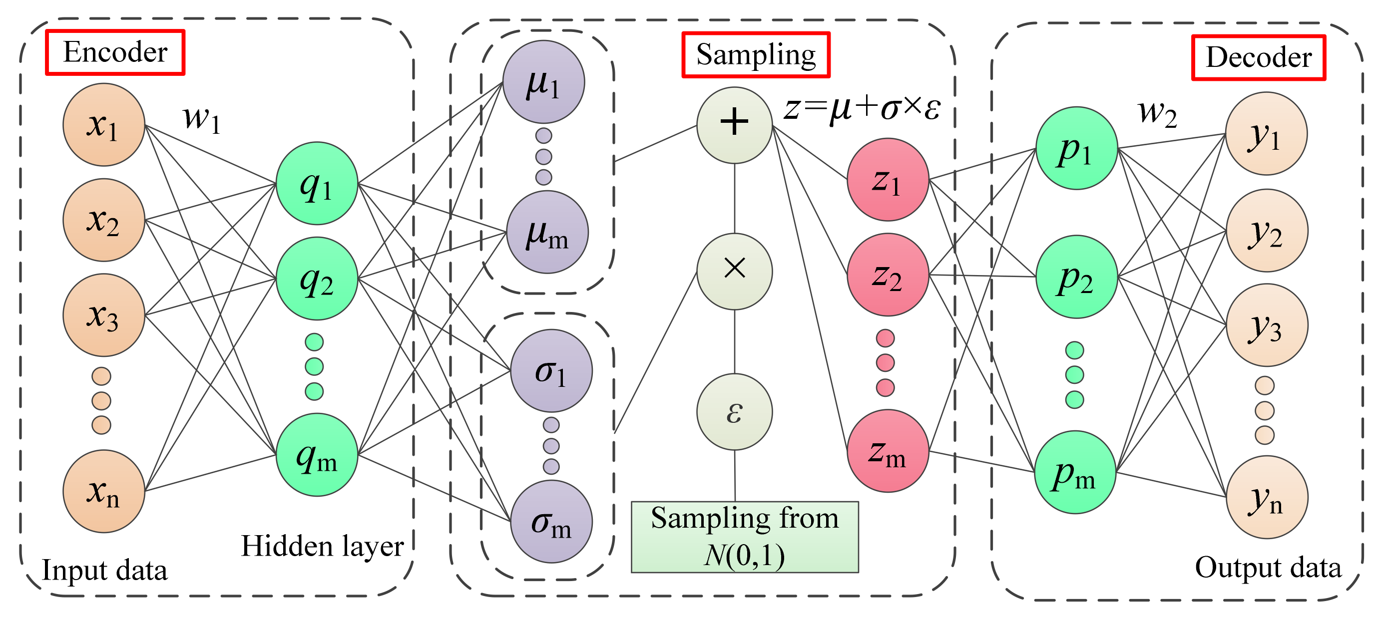
2.1. Overview of Variational Auto-Encoder
2.2. Literature Review on Variational Auto-Encoder in Fault Diagnosis
- (1)
- To improve the anti-noise capability of VAE model, a new deep learning model, named stacked variational denoising auto-encoder (SVDAE), is constructed by integrating stacked denoising techniques and a variational auto-encoder.
- (2)
- To avoid the dependence of human experience of parameter selection of the existing VAE model, we adopted a novel optimizer, the seagull optimization algorithm (SOA), using its fast operation to adaptively select the parameters of SVDAE.
- (3)
- To improve the accuracy of fault diagnosis, an intelligent diagnosis scheme based on optimized stacked variational denoising autoencoder (OSVDAE) is proposed that can effectively identify bearing faults under constant and variable speeds.
3. Proposed Methodologies
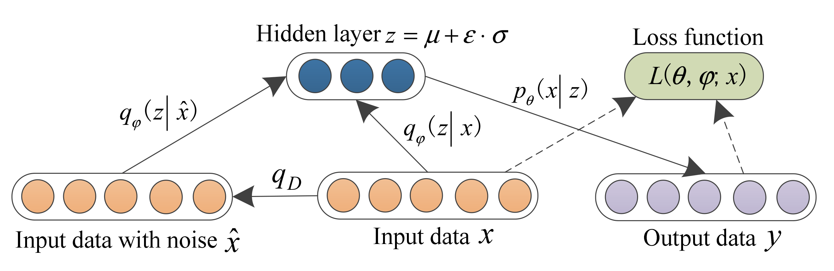
3.1. Variational Denoising Auto-Encoder
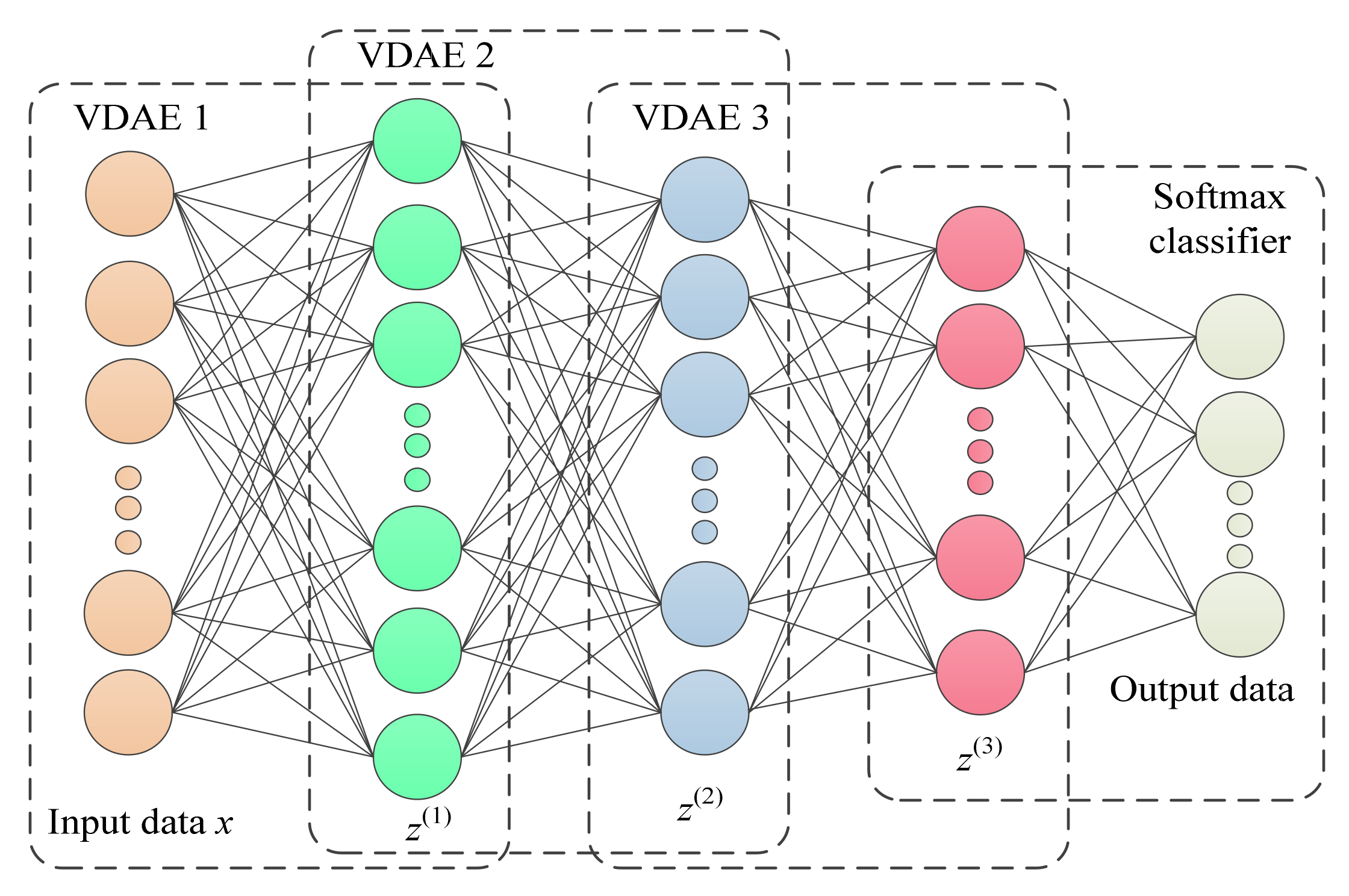
3.2. Stacked Variational Denoising Auto-Encoder
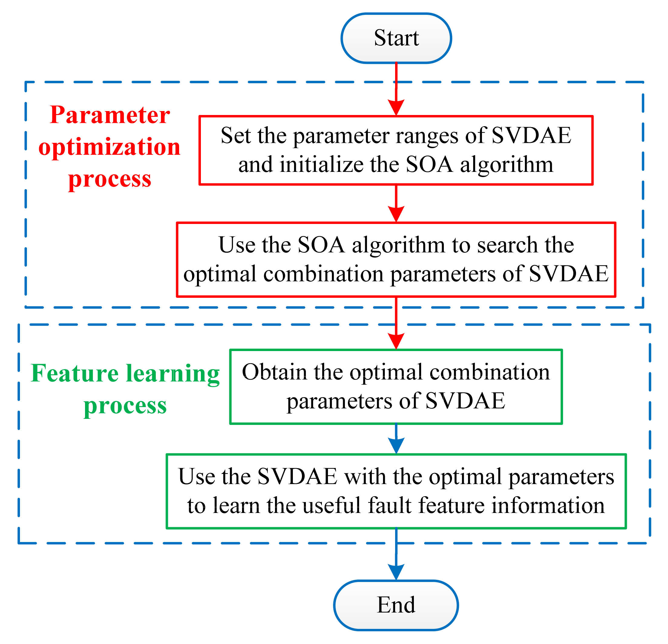
3.3. Optimized Stacked Variational Denoising Auto-Encoder
- (1)
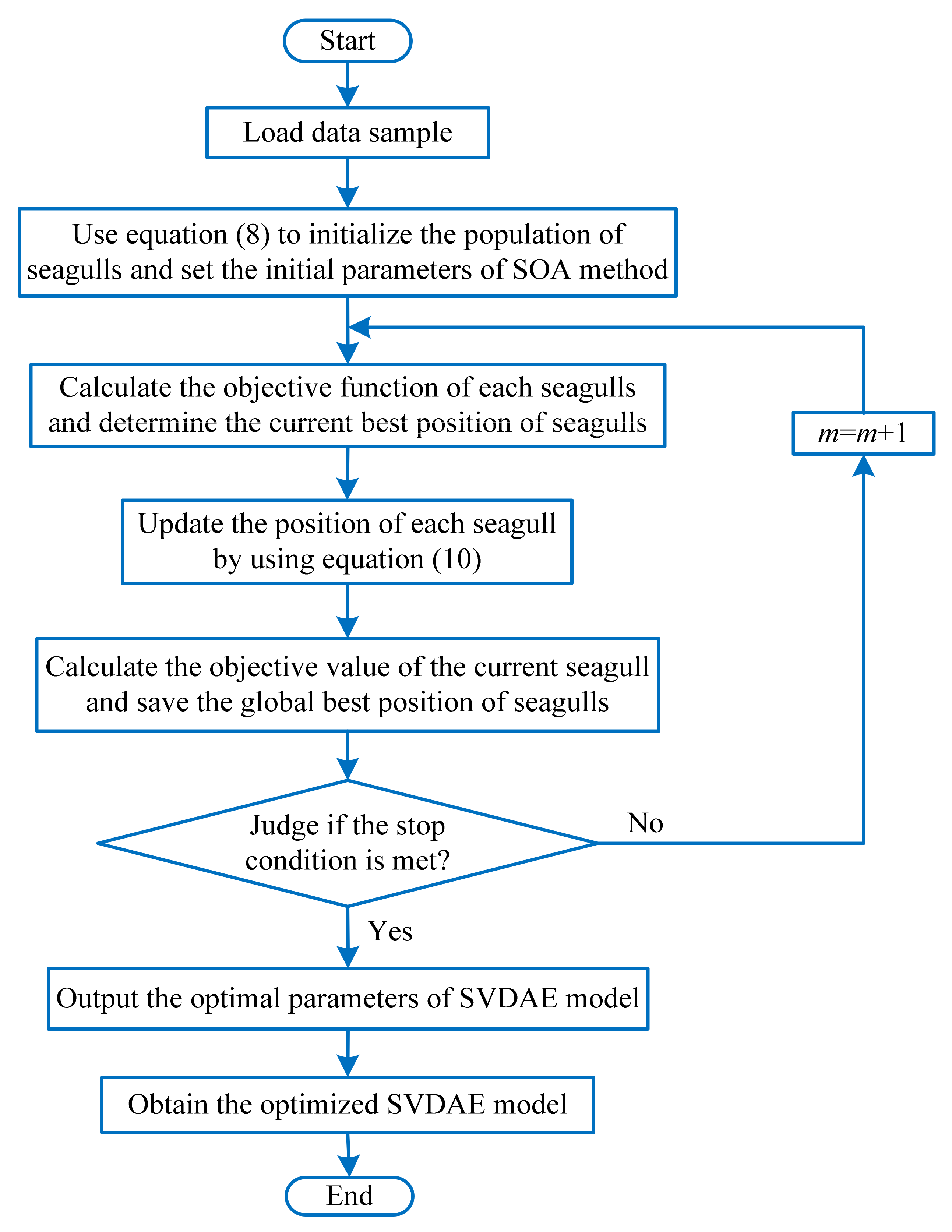
- Load sample data, use Equation (8) to initialize the population of seagulls and set the initial parameters of the SOA. Specifically, set the population size of seagulls N = 100, maximum number of iterations = 200, the frequency coefficient = 2, the current iteration number and the constants Considering there are five variables in the SVDAE model that need to be optimized, the position of each seagull is expressed by a vector where represents the learning rate of each VDAE, N denotes the epochs number of the SVDAE model, l1, l2 and l3 are the number of nodes of the hidden layers of VDAE1, VDAE2 and VDAE3, respectively.where = [10, 0.001, 400, 200, 50] and = [200, 1, 800, 400, 100] represent the upper and lower bounds of the vector respectively.
- (2)
- Calculate the objective function of each seagull and determine the current best position of the seagulls. In this step, the identification accuracy is selected as the objective function, as shown in Equation (9).where denotes the number of misidentified samples, and is the number of correctly identified samples.
- (3)
- According to Equation (10), calculate the distance between the current seagull and the best seagull, and update the position of each seagull.where denotes the current position in the updating of seagulls, denotes the current best position in the updating of seagulls and x denotes the current iteration number. represents the distance between the current seagull and the best seagull, represents the current seagull position that will not collide with other seagulls, A represents the movement behavior of seagulls in a given search space and meets , is a frequency coefficient that can control the variation range of the variable A, which is linearly decreased from to 0, and . denotes the position of each seagull moving towards the best seagull, B is a random number and satisfies , is a random number between 0 and 1. , and are all plane coordinates, while represents the radius of each turn of the spiral, and are constants that controls the shape of the spiral and k denotes a random number between 0 and .
- (4)
- Calculate the objective value of the current seagull and save the global best position of the seagulls. If is better than , is considered as the global best position of the seagulls. Otherwise, is considered the individual best position of seagulls from which to continue to update.
- (5)
- Judge if the stop condition is met. Specifically, judge whether the number of iterations is reached or the expected identification accuracy is achieved. If it reaches maximum number of iterations, output the best position of the seagulls (i.e., the optimal combination parameters of the SVDAE model). Otherwise, set m = m + 1, repeat the steps (2)~(5) until the stop condition is satisfied.
- (6)
- Use the optimized SVDAE model to automatically learn the discriminative fault feature information from the collected bearing vibration signal.
3.4. Proposed OSVDAE-Based Fault Diagnosis Method
4. Experimental Verification and Discussion
4.1. Case 1: Bearing Experimental Data from CWRU
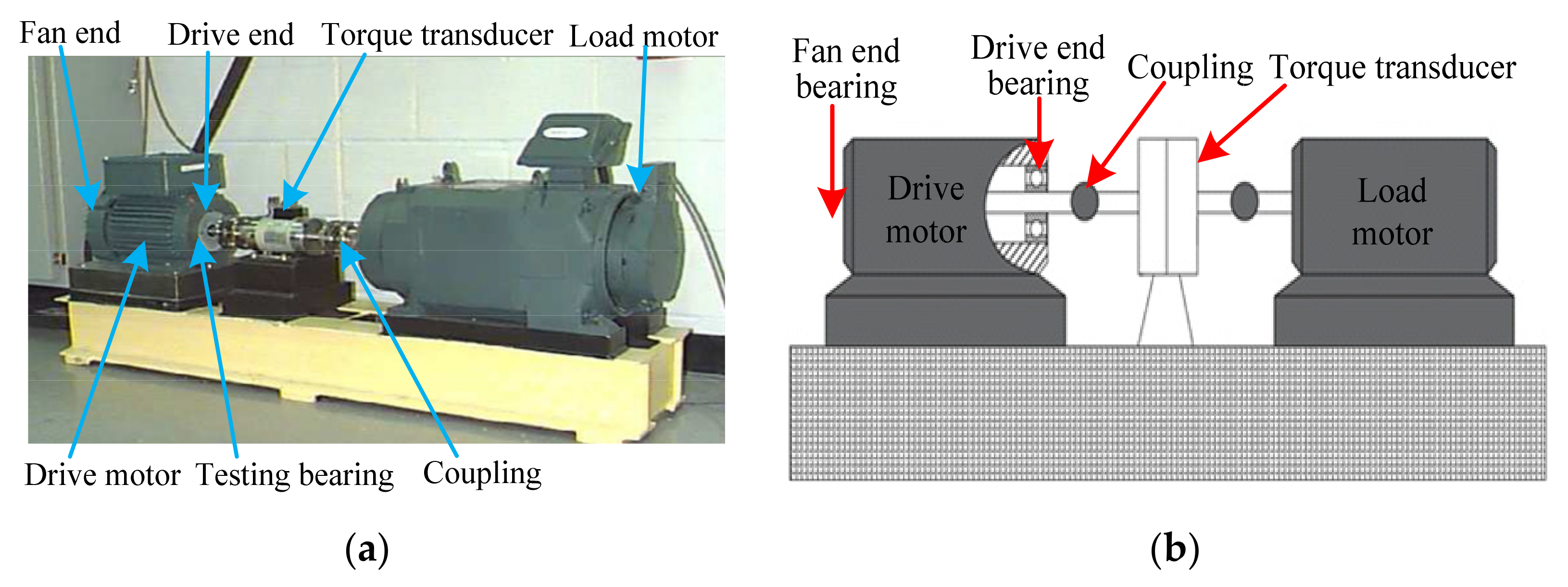
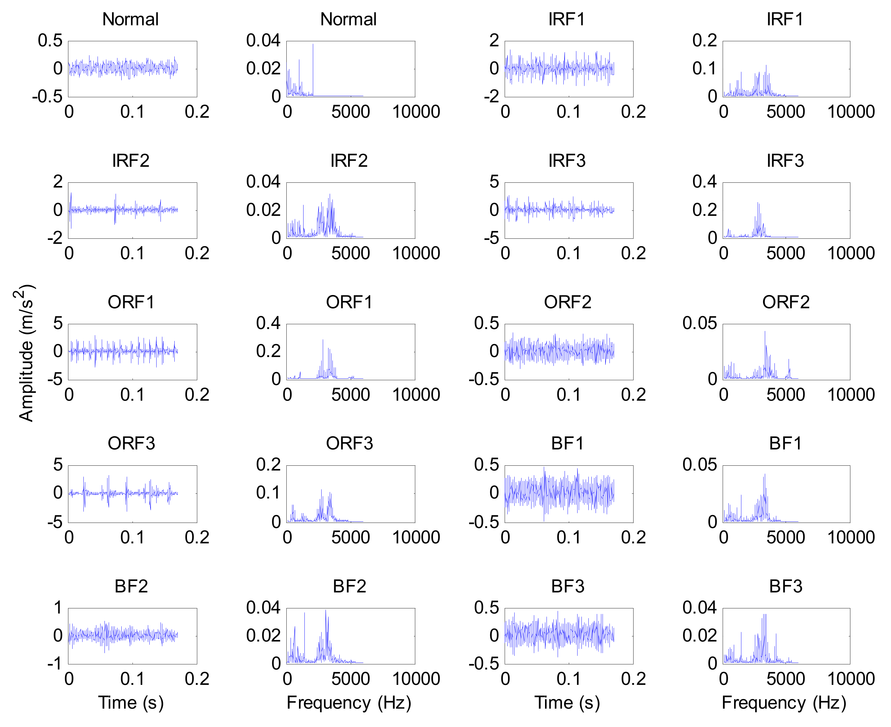
4.1.1. Data Description and Settings
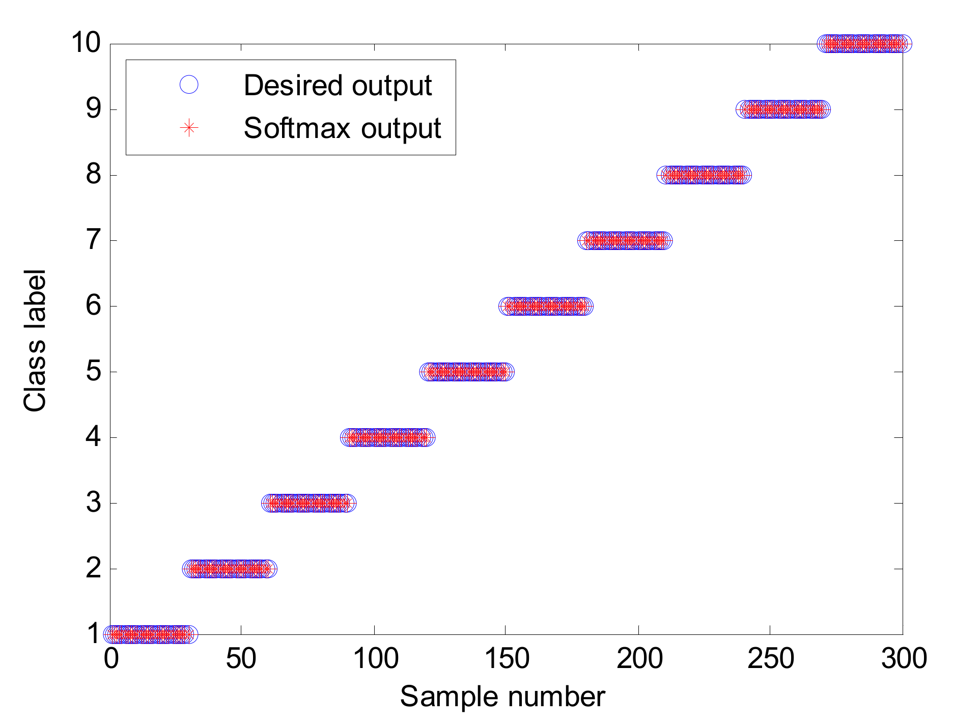
4.1.2. Results and Analysis of Fault Diagnosis
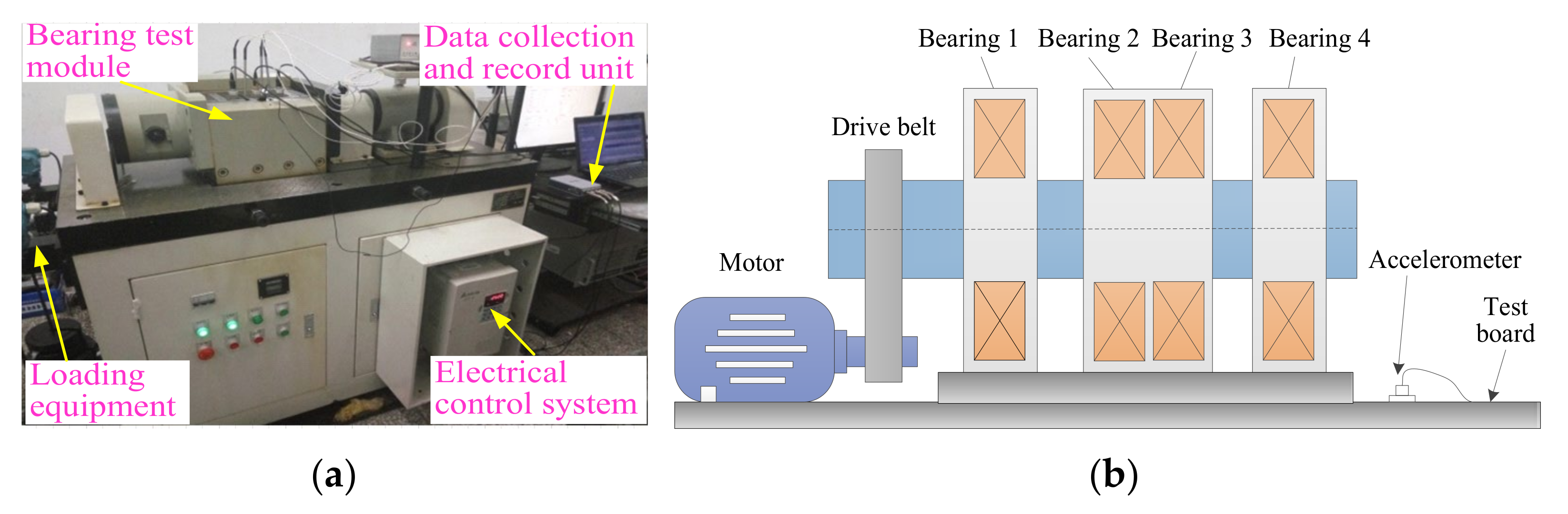
4.2. Case 2: Bearing Vibration Data from Laboratory
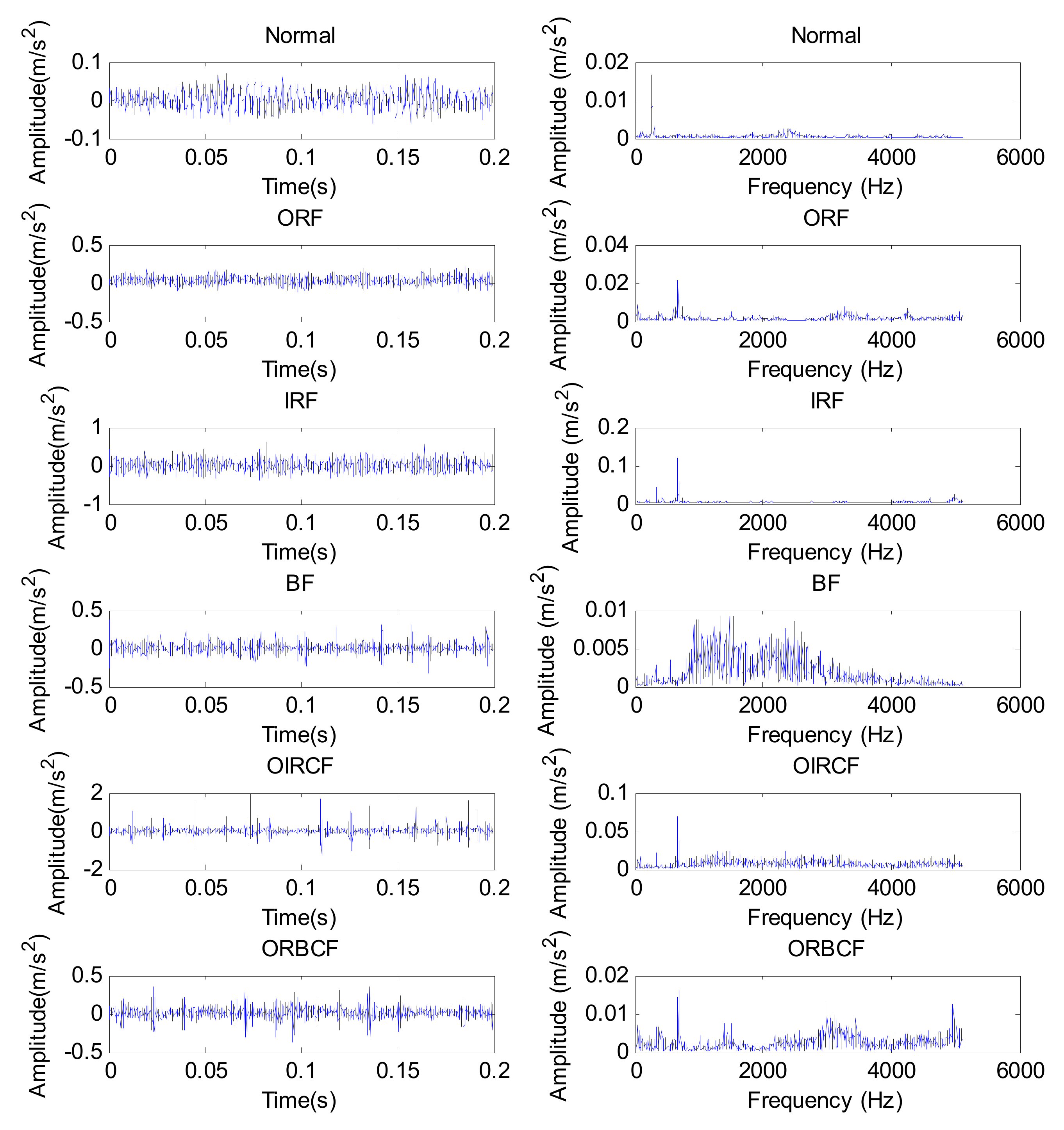
4.2.1. Data Description and Settings
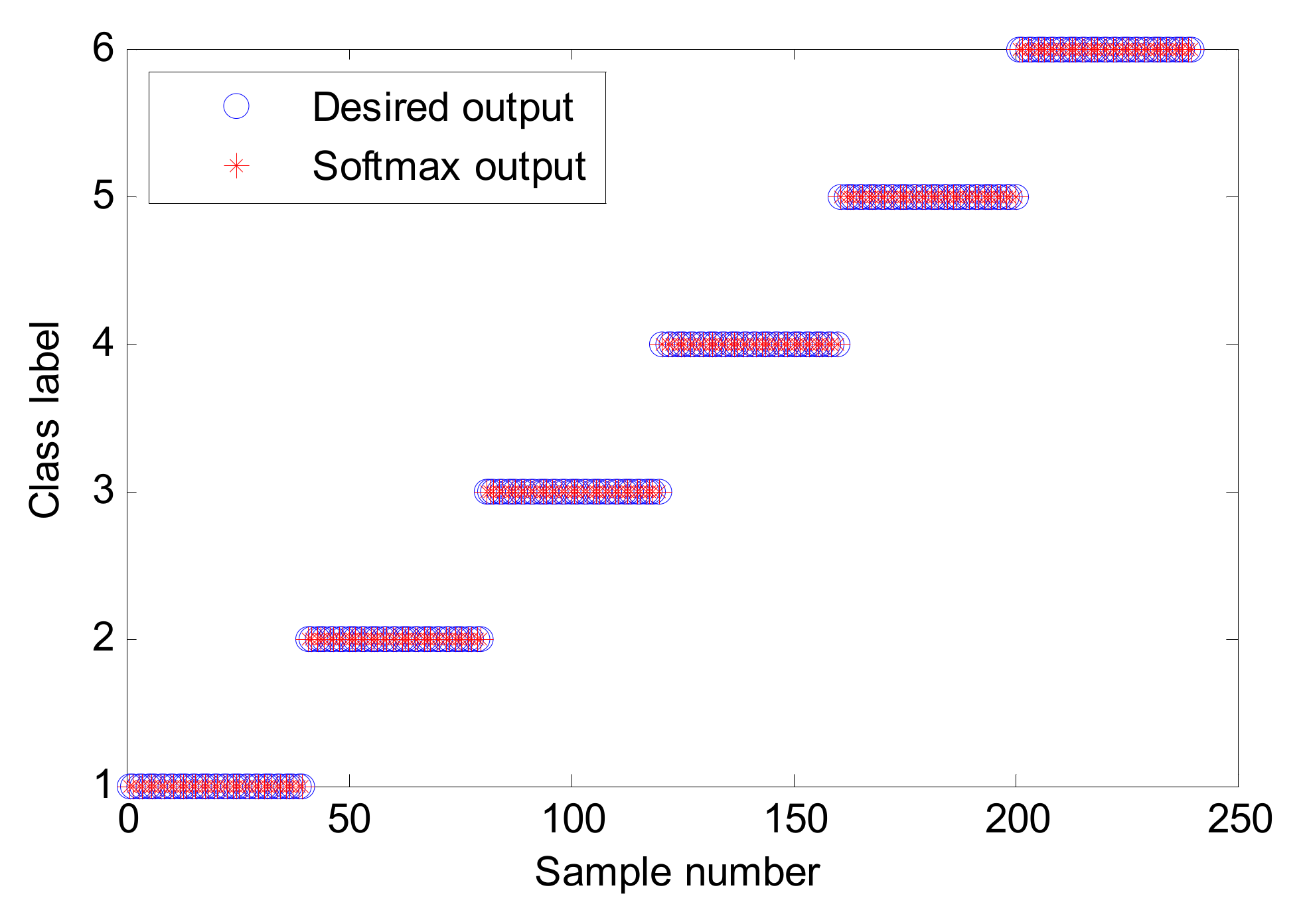
4.2.2. Results and Analysis of Fault Diagnosis
4.3. Research Limitations and Future Work
- (1)
- In this paper, through the fusion of stacked denoising techniques, VAE and an optimization algorithm, the proposed method could improve the anti-noise performance of the VAE model and adaptively select its parameters. However, the over-fitting problem of the proposed method was not considered completely. That is, the overfitting problem of the network model is one limitation of this study. Therefore, to solve this problem, in a future work, considering the advantages of the existing available advanced AE (e.g., deep sparse auto-encoder [34], deep contractive auto-encoder [35], deep convolutional auto-encoder [36], wavelet auto-encoder (WAE) [37], and discriminative manifold regularized auto-encoder (DMRAE) [38]), we intend to add a sparsity constraint to the neurons in the hidden layer of the SVDAE and improve the loss function of the SVDAE by adding the Jacobian norm to develop an ensemble stacked variational auto-encoder (ESVAE) that can both prevent over-fitting and improve feature-learning ability.
- (2)
- It is difficult to obtain sufficient bearing fault data in actual production, which easily leads to imbalanced samples from training. This indicates that bearing fault diagnosis, under data imbalance, is a difficult problem. That is, another limitation of this study is the uncertainty of implementing unbalanced bearing fault diagnosis. Therefore, to solve the unbalanced fault diagnosis problem, in a future work, we intend to integrate the synthetic minority over-sampling technique or bagging method into SVDAE to improve the generalization performance of the network model. Additionally, some loss items (e.g., the focal loss, piecewise loss) can also be added into the SVDAE model to solve the unbalanced fault diagnosis problem of rolling bearings, which is our future research direction.
- (3)
- When multi-sensor experimental data are collected, including vibration and acoustic signals, the utilization of multi-sensor information is very critical for the reliable fault diagnosis of bearings. This paper mainly solves the bearing fault diagnosis problem of single-sensor data, whereas the effectiveness of the proposed method is unknown for multi-sensor data processing. That is, the indeterminacy of the proposed method in multi-sensor fault diagnosis is regarded as one limitation of this study. Therefore, in our future work, we will refer to the coupling notion of a deep coupling auto-encoder (DCAE) [39], by which the proposed method can be improved to handle multi-sensor data, aimed at capturing the joint fault feature information between multi-sensor signals and perform more accurate fault diagnosis.
- (4)
- In the experimental case 2 of this paper, bearing vibration data were actually collected on different dates. As the room temperature was different on different dates, the collected bearing vibration data was collected in different room temperatures. This indicates that the proposed method can identify bearing faults under different room temperatures. In other words, when bearing vibration data of different room temperatures are analyzed, it is generally not required to re-train the proposed model. However, due to the limitations of the experimental conditions, when the experiments of this paper were conducted, the room temperatures were not recorded, which is regarded as one deficiency of this study. Therefore, in our future work, we will adopt a thermodetector to record the room temperature in which bearing data is collected and confirm the identification accuracy of the proposed method as a function of room temperature.
- (5)
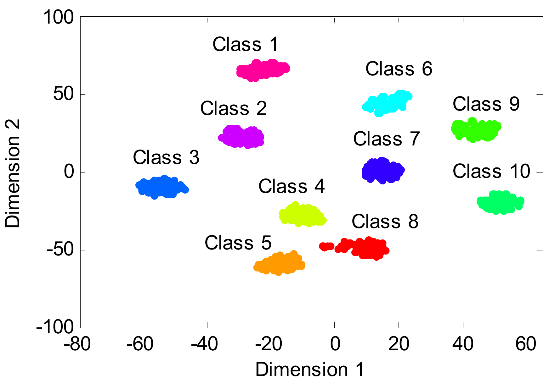
- In two experimental cases of this paper, the robustness and parameter selection of the proposed SVDAE were studied intensively, but the internal working mechanism of the SVDAE was not investigated in detail. Therefore, in our future work, we will adopt some representative feature visualization techniques (e.g., t-distributed stochastic neighbor embedding (t-SNE), principal component analysis (PCA), local preserving projection (LPP) and local sensitive discriminant analysis (LSDA)) to clearly describe the clustering of output features of the different layers of SVDAE. Meanwhile, in a future work, the discrimination degree of the output features of the proposed method will be quantitatively evaluated by using sensitive indexes (e.g., intra-class distance, inter-class distance and the ratio between them).
5. Conclusions
- (1)
- A novel deep learning model, named stacked variational denoising auto-encoder (SVDAE), was presented to extract the inherent fault features from the original bearing vibration data and provided better robustness than the original VAE.
- (2)
- A new meta-heuristic intelligent optimizer, termed the seagull optimization algorithm (SOA), was employed to automatically select the hyper-parameters of SVDAE model, which improved the feature learning ability and avoided the dependence upon human experience for parameter selection in deep learning.
- (3)
- An intelligent diagnostic framework based on optimized stacked variational denoising autoencoder (OSVDAE) was proposed for reliably diagnosing bearing faults that does not require artificial, features-based expert knowledge and so is appropriate for ordinary technicians.
- (4)
- The experimental results and comparison analysis of bearing fault diagnosis showed the effectiveness and superiority of the proposed method.
Author Contributions
Funding
Institutional Review Board Statement
Informed Consent Statement
Data Availability Statement
Acknowledgments
Conflicts of Interest
References
- Yan, X.; Liu, Y.; Xu, Y.; Jia, M. Multichannel fault diagnosis of wind turbine driving system using multivariate singular spectrum decomposition and improved Kolmogorov complexity. Renew. Energy 2021, 170, 724–748. [Google Scholar] [CrossRef]
- Li, Y.; Zeng, Y.; Qing, Y.; Huang, G. Learning local discriminative representations via extreme learning machine for machine fault diagnosis. Neurocomputing 2020, 409, 275–285. [Google Scholar] [CrossRef]
- Yan, X.; Liu, Y.; Jia, M. A fault diagnosis approach for rolling bearing integrated SGMD, IMSDE and multiclass relevance vector machine. Sensors 2020, 20, 4352. [Google Scholar] [CrossRef] [PubMed]
- Kuvvetli, Y.; Deveci, M.; Paksoy, T.; Garg, H. A predictive analytics model for COVID-19 pandemic using artificial neural networks. Decis. Anal. J. 2021, 1, 100007. [Google Scholar] [CrossRef]
- Gunerkar, R.; Jalan, A.; Belgamwar, S. Fault diagnosis of rolling element bearing based on artificial neural network. J. Meas. Sci. Technol. 2019, 33, 505–511. [Google Scholar] [CrossRef]
- Jin, H.; Titus, A.; Liu, Y.; Wang, Y.; Han, A. Fault diagnosis of rotary parts of a heavy-duty horizontal lathe based on wavelet packet transform and support vector machine. Sensors 2019, 19, 4069. [Google Scholar] [CrossRef] [Green Version]
- Li, K.; Su, L.; Wu, J.; Wang, H.; Chen, P. A rolling bearing fault diagnosis method based on variational mode decomposition and an improved kernel extreme learning machine. Appl. Sci. 2017, 7, 1004. [Google Scholar] [CrossRef] [Green Version]
- Li, W.; Luo, Z.; Jin, Y.; Xi, X. Gesture recognition based on multiscale singular value entropy and deep belief network. Sensors 2020, 21, 119. [Google Scholar] [CrossRef]
- Liu, P.; Yang, X.; Jin, B.; Zhou, Q. Diabetic retinal grading using attention-based bilinear convolutional neural network and complement cross entropy. Entropy 2021, 23, 816. [Google Scholar] [CrossRef]
- Zhou, H.; Zhuang, Z.; Liu, Y.; Liu, Y.; Zhang, X. Defect classification of green plums based on deep learning. Sensors 2020, 20, 6993. [Google Scholar] [CrossRef]
- Yan, X.; Liu, Y.; Jia, M. Health condition identification for rolling bearing using a multi-domain indicator-based optimized stacked denoising autoencoder. Struct. Health Monit. 2020, 19, 1602–1626. [Google Scholar] [CrossRef]
- Shao, H.; Jiang, H.; Wang, F.; Wang, Y. Rolling bearing fault diagnosis using adaptive deep belief network with dual-tree complex wavelet packet. ISA Trans. 2017, 69, 187–201. [Google Scholar] [CrossRef]
- Liu, Y.; Yan, X.; Zhang, C.; Liu, W. An ensemble convolutional neural networks for bearing fault diagnosis using multi-sensor data. Sensors 2019, 19, 5300. [Google Scholar] [CrossRef] [Green Version]
- Zhang, Y.; Li, X.; Gao, L.; Chen, W.; Li, P. Ensemble deep contractive auto-encoders for intelligent fault diagnosis of machines under noisy environment. Knowl.-Based Syst. 2020, 196, 105764. [Google Scholar] [CrossRef]
- Kingma, D.; Welling, M. Auto-encoding variational bayes. arXiv 2013, arXiv:1312.6114v10. [Google Scholar]
- Yan, X.; She, D.; Xu, Y.; Jia, M. Deep regularized variational autoencoder for intelligent fault diagnosis of rotor-bearing system within entire life-cycle process. Knowl.-Based Syst. 2021, 226, 107142. [Google Scholar] [CrossRef]
- Dhiman, G.; Kumar, V. Seagull optimization algorithm: Theory and its applications for large-scale industrial engineering problems. Knowl.-Based Syst. 2019, 165, 169–196. [Google Scholar] [CrossRef]
- Demirel, N.; Deveci, M. Novel search space updating heuristics-based genetic algorithm for optimizing medium-scale airline crew pairing problems. Int. J. Comput. Int. Syst. 2017, 10, 1082–1101. [Google Scholar] [CrossRef] [Green Version]
- Chen, K.; Mao, Z.; Zhao, H.; Jiang, Z.; Zhang, J. A variational stacked autoencoder with harmony search optimizer for valve train fault diagnosis of diesel engine. Sensors 2019, 20, 223. [Google Scholar] [CrossRef] [Green Version]
- Huang, Y.; Chen, C.; Huang, C. Motor fault detection and feature extraction using rnn-based variational autoencoder. IEEE Access 2019, 7, 139086–139096. [Google Scholar] [CrossRef]
- Martin, G.; Droguett, E.; Meruane, V.; Moura, M. Deep variational auto-encoders: A promising tool for dimensionality reduction and ball bearing elements fault diagnosis. Struct. Health Monit. 2019, 18, 1092–1128. [Google Scholar] [CrossRef]
- Zhao, D.; Liu, S.; Gu, D.; Sun, X.; Wang, L.; Wei, Y.; Zhang, H. Enhanced data-driven fault diagnosis for machines with small and unbalanced data based on variational auto-encoder. Meas. Sci. Technol. 2020, 31, 35004. [Google Scholar] [CrossRef]
- Wang, Y.; Sun, G.; Jin, Q. Imbalanced sample fault diagnosis of rotating machinery using conditional variational auto-encoder generative adversarial network. Appl. Soft Comput. 2020, 92, 106333. [Google Scholar] [CrossRef]
- Yan, K.; Su, J.; Huang, J.; Mo, Y. Chiller fault diagnosis based on VAE-enabled generative adversarial networks. IEEE Trans. Autom. Sci. Eng. 2020, 1–9. [Google Scholar] [CrossRef]
- Tang, P.; Peng, K.; Dong, J. Nonlinear quality-related fault detection using combined deep variational information bottleneck and variational autoencoder. ISA Trans. 2021, 114, 444–454. [Google Scholar] [CrossRef]
- Costa, N.; Sanchez, L.; Couso, I. Semi-supervised recurrent variational autoencoder approach for visual diagnosis of atrial fibrillation. IEEE Access 2021, 9, 40227–40239. [Google Scholar] [CrossRef]
- Kim, Y.; Lee, H.; Kim, C. A variational autoencoder for a semiconductor fault detection model robust to process drift due to incomplete maintenance. J. Intell. Manuf. 2021, 1–12. [Google Scholar] [CrossRef]
- Zhang, S.; Ye, F.; Wang, B.; Habetler, G. Semi-Supervised Bearing fault diagnosis and classification using variational autoencoder-based deep generative models. IEEE Sens. J. 2021, 21, 6476–6486. [Google Scholar] [CrossRef]
- Chao, M.; Adey, B.; Fink, O. Implicit supervision for fault detection and segmentation of emerging fault types with deep variational autoencoders. Neurocomputing 2021, 454, 324–338. [Google Scholar] [CrossRef]
- Che, L.; Yang, X.; Wang, L. Text feature extraction based on stacked variational autoencoder. Microprocess. Microsyst. 2020, 76, 103063. [Google Scholar] [CrossRef]
- Chen, Z.; Li, Z.; Li, C.; Valente, D. Fault diagnosis method of rotating machinery based on stacked denoising autoencoder. J. Intell. Fuzzy Syst. 2018, 34, 3443–3449. [Google Scholar] [CrossRef]
- Shang, Z.; Liao, X.; Geng, R.; Gao, M.; Liu, X. Fault diagnosis method of rolling bearing based on deep belief network. J. Mech. Sci. Technol. 2018, 32, 5139–5145. [Google Scholar] [CrossRef]
- Appana, D.; Alexander, P.; Jong-Myon, K. Reliable fault diagnosis of bearings with varying rotational speeds using envelope spectrum and convolution neural networks. Soft Comput. 2018, 22, 6719–6729. [Google Scholar] [CrossRef]
- Qi, Y.; Shen, C.; Dong, W.; Shi, J.; Zhu, Z. Stacked sparse autoencoder-based deep network for fault diagnosis of rotating machinery. IEEE Access 2017, 5, 15066–15079. [Google Scholar] [CrossRef]
- Aamir, M.; Nawi, N.; Wahid, F.; Mahdin, H. A deep contractive autoencoder for solving multiclass classification problems. Evol. Intel. 2021, 14, 1619–1633. [Google Scholar] [CrossRef]
- Chen, S.; Yu, J.; Wang, S. One-dimensional convolutional auto-encoder-based feature learning for fault diagnosis of multivariate processes. J. Process Contr. 2020, 87, 54–67. [Google Scholar] [CrossRef]
- Shao, H.; Jiang, H.; Li, X.; Wu, S. Intelligent fault diagnosis of rolling bearing using deep wavelet auto-encoder with extreme learning machine. Knowl.-Based Syst. 2017, 140, 1–14. [Google Scholar]
- Farajian, N.; Adibi, P. DMRAE: Discriminative manifold regularized auto-encoder for sparse and robust feature learning. Progress Artif. Intell. 2020, 9, 263–274. [Google Scholar] [CrossRef]
- Ma, M.; Sun, C.; Chen, X. Deep coupling autoencoder for fault diagnosis with multimodal sensory data. IEEE Trans. Ind. Inform. 2018, 14, 1137–1145. [Google Scholar] [CrossRef]


| Authors | Year | Country/Region | Research Problem | Methods | Experiment Validation (Yes/No) | Data Access |
|---|---|---|---|---|---|---|
| Chen et al. | 2019 | China | fault diagnosis of diesel engine | VSAE | yes | private |
| Huang et al. | 2019 | Taiwan | motor fault detection | RNN-based VAE | yes | private |
| Martin et al. | 2019 | Chile | bearing fault diagnosis | Deep VAE | yes | public |
| Zhao et al. | 2020 | China | bearing fault diagnosis | VAE and CNN | yes | private |
| Wang et al. | 2020 | China | fault diagnosis of planetary gearbox | CVAE-GAN | yes | private |
| Yan et al. | 2020 | China and Singapore | chiller fault diagnosis | CWGAN-GP-VAE | yes | private |
| Tang et al. | 2021 | China | quality-related fault detection | VAE and VIB | yes | private |
| Costa et al. | 2021 | Spain | visual diagnosis of atrial fibrillation | RVAE | yes | private |
| Kim et al. | 2021 | Republic of Korea | semiconductor fault detection | VAE model | yes | private |
| Zhang et al. | 2021 | USA | bearing fault diagnosis | VAE-based deep generative models | yes | public |
| Chao et al. | 2021 | Switzerland | fault diagnosis of safety-critical systems | KIL-AdaVAE | yes | public |
| Bearing Type | Roller Diameter (mm) | Pitch Diameter (mm) | Number of Balls | Contact Angle (o) |
|---|---|---|---|---|
| SKF6205-2RS | 7.94 | 39.04 | 9 | 0 |
| Bearing Condition | Motor Speed (rpm) | Fault Diameter (mils) | Number of Training Samples | Number of Testing Samples | Class Label |
|---|---|---|---|---|---|
| Normal | 1730 | 0 | 30 | 30 | 1 |
| Inner race fault 1 (IRF1) | 1750 | 7 | 30 | 30 | 2 |
| Inner race fault 2 (IRF2) | 1750 | 14 | 30 | 30 | 3 |
| Inner race fault 3 (IRF3) | 1750 | 21 | 30 | 30 | 4 |
| Outer race fault 1 (ORF1) | 1772 | 7 | 30 | 30 | 5 |
| Outer race fault 2 (ORF2) | 1772 | 14 | 30 | 30 | 6 |
| Outer race fault 3 (ORF3) | 1772 | 21 | 30 | 30 | 7 |
| Ball fault 1 (BF1) | 1797 | 7 | 30 | 30 | 8 |
| Ball fault 2 (BF2) | 1797 | 14 | 30 | 30 | 9 |
| Ball fault 3 (BF3) | 1797 | 21 | 30 | 30 | 10 |
| Model Parameters | Value |
|---|---|
| The number of iterations N | 180 |
| The learning rate a | 0.009 |
| The number of nodes in the first hidden layer l1 | 660 |
| The number of nodes in the second hidden layer l2 | 250 |
| The number of nodes in the third hidden layer l3 | 80 |
| Different Methods | Identification Accuracy Obtained Using Different Methods (%) | |||
|---|---|---|---|---|
| Maximum | Minimum | Mean | Standard Deviation | |
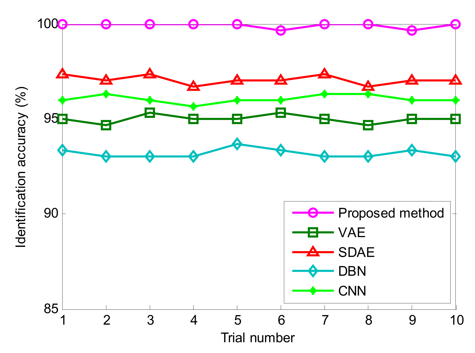
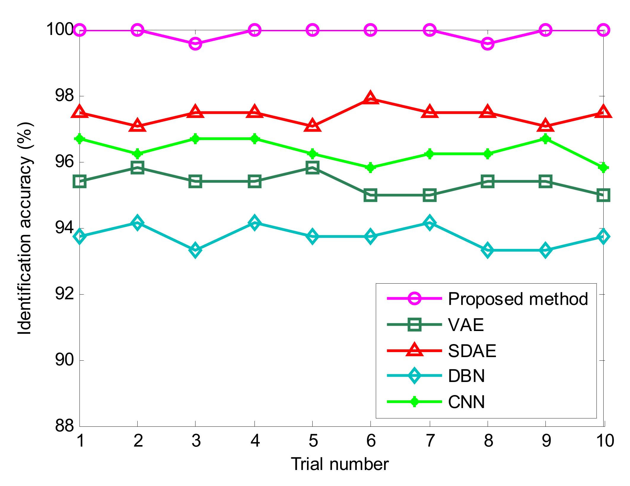
| Proposed method | 100 | 99.67 | 99.93 | 0.1391 |
| VAE | 95.33 | 94.67 | 95.00 | 0.2200 |
| SDAE | 97.33 | 96.67 | 97.03 | 0.2435 |
| DBN | 93.67 | 93.00 | 93.17 | 0.2357 |
| CNN | 96.33 | 95.67 | 96.06 | 0.2087 |
| Different Methods | Accuracy Obtained by Different Methods for Five Trials (%) | Average Accuracy (%) | ||||
|---|---|---|---|---|---|---|
| 1 | 2 | 3 | 4 | 5 | ||
| Proposed method | 100 | 100 | 99.17 | 100 | 100 | 99.83 |
| VAE | 95.83 | 95.00 | 95.83 | 95.83 | 95.00 | 95.49 |
| SDAE | 97.50 | 97.50 | 96.67 | 96.67 | 97.50 | 97.16 |
| DBN | 93.33 | 92.50 | 93.33 | 93.33 | 92.50 | 92.99 |
| CNN | 96.67 | 96.67 | 95.83 | 96.67 | 95.83 | 96.33 |
| Bearing Type | Ball Diameter (mm) | Pitch Diameter (mm) | Number of Balls | Contact Angle (°) |
|---|---|---|---|---|
| HRB6205 | 7.94 | 39.04 | 9 | 0 |
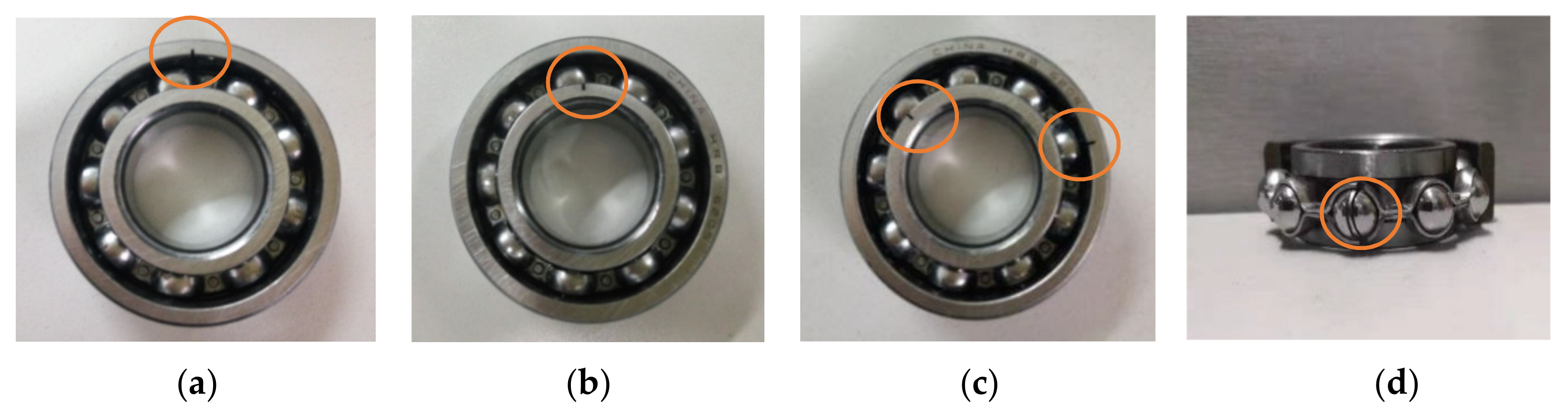
| Bearing Conditions | Fault Diameter (Width × Depth) | Number of Training Samples | Number of Testing Samples | Class Labels |
|---|---|---|---|---|
| Normal | 0 × 0 mm | 40 | 40 | 1 |
| Outer race fault (ORF) | 0.1 × 0.6 mm | 40 | 40 | 2 |
| Inner race fault (IRF) | 0.1 × 0.5 mm | 40 | 40 | 3 |
| Ball fault (BF) | 0.1 × 0.6 mm | 40 | 40 | 4 |
| Outer and inner race compound fault (OIRCF) | 0.1 × 0.5 mm | 40 | 40 | 5 |
| Outer race and ball compound fault (ORBCF) | 0.1 × 0.6 mm | 40 | 40 | 6 |
| Model Parameters | Value |
|---|---|
| The number of iterations N | 150 |
| The learning rate a | 0.003 |
| The number of nodes in the first hidden layer l1 | 580 |
| The number of nodes in the second hidden layer l2 | 270 |
| The number of nodes in the third hidden layer l3 | 60 |
| Different Methods | Identification Accuracy Obtained Using Different Methods (%) | |||
|---|---|---|---|---|
| Maximum | Minimum | Mean | Standard Deviation | |
| Proposed method | 100 | 99.58 | 99.91 | 0.1771 |
| VAE | 95.83 | 95.00 | 95.37 | 0.3058 |
| SDAE | 97.91 | 97.08 | 97.41 | 0.2635 |
| DBN | 94.16 | 93.33 | 93.74 | 0.3389 |
| CNN | 96.67 | 95.83 | 96.33 | 0.3313 |
| Different Methods | Accuracy Obtained by Different Methods for Five Trials (%) | Average Accuracy (%) | ||||
|---|---|---|---|---|---|---|
| 1 | 2 | 3 | 4 | 5 | ||
| Proposed method | 100 | 100 | 98.95 | 100 | 100 | 99.79 |
| VAE | 95.83 | 95.83 | 94.79 | 94.79 | 95.83 | 95.41 |
| SDAE | 97.91 | 96.87 | 97.91 | 97.91 | 96.87 | 97.49 |
| DBN | 93.75 | 93.75 | 92.71 | 92.71 | 93.75 | 93.33 |
| CNN | 96.87 | 95.83 | 96.87 | 96.87 | 95.83 | 96.45 |
Publisher’s Note: MDPI stays neutral with regard to jurisdictional claims in published maps and institutional affiliations. |
© 2021 by the authors. Licensee MDPI, Basel, Switzerland. This article is an open access article distributed under the terms and conditions of the Creative Commons Attribution (CC BY) license (https://creativecommons.org/licenses/by/4.0/).
Share and Cite
Yan, X.; Xu, Y.; She, D.; Zhang, W. Reliable Fault Diagnosis of Bearings Using an Optimized Stacked Variational Denoising Auto-Encoder. Entropy 2022, 24, 36. https://doi.org/10.3390/e24010036
Yan X, Xu Y, She D, Zhang W. Reliable Fault Diagnosis of Bearings Using an Optimized Stacked Variational Denoising Auto-Encoder. Entropy. 2022; 24(1):36. https://doi.org/10.3390/e24010036
Chicago/Turabian StyleYan, Xiaoan, Yadong Xu, Daoming She, and Wan Zhang. 2022. "Reliable Fault Diagnosis of Bearings Using an Optimized Stacked Variational Denoising Auto-Encoder" Entropy 24, no. 1: 36. https://doi.org/10.3390/e24010036