
Synchronizing Two Superconducting Qubits through a Dissipating Resonator


Abstract
:1. Introduction
2. The Model
2.1. Hamiltonian and Dissipators
2.2. Conservation of the Excitation Number
3. Protected States and Qubit Synchronization
3.1. Theoretical Analysis
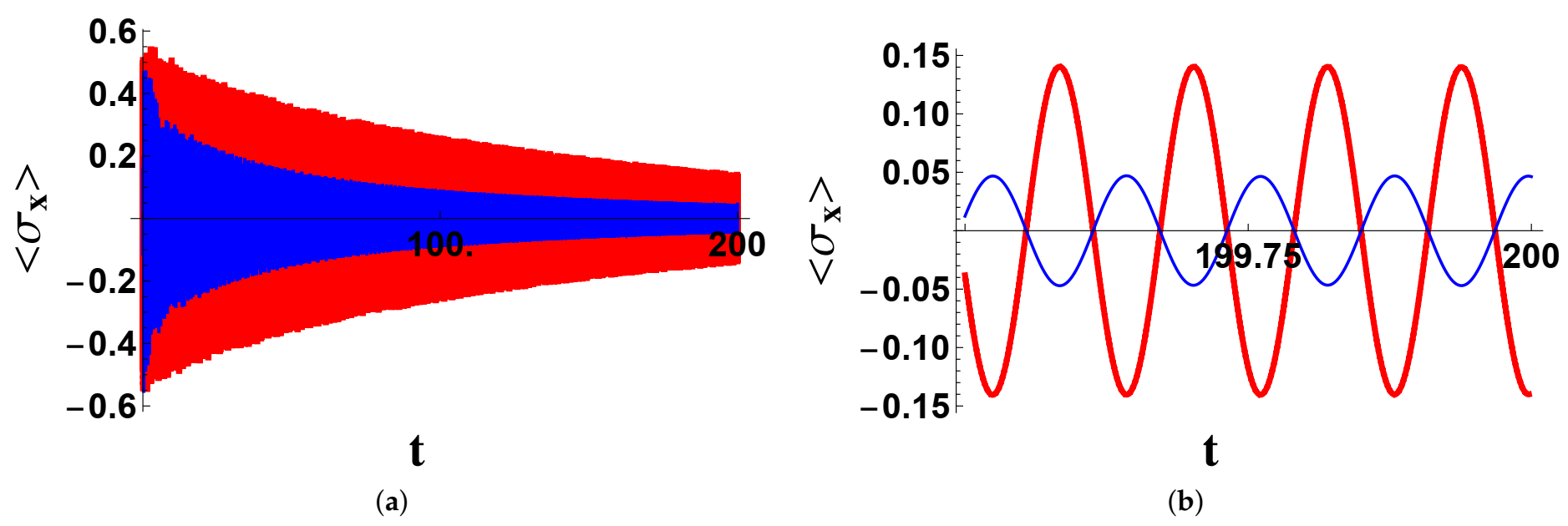
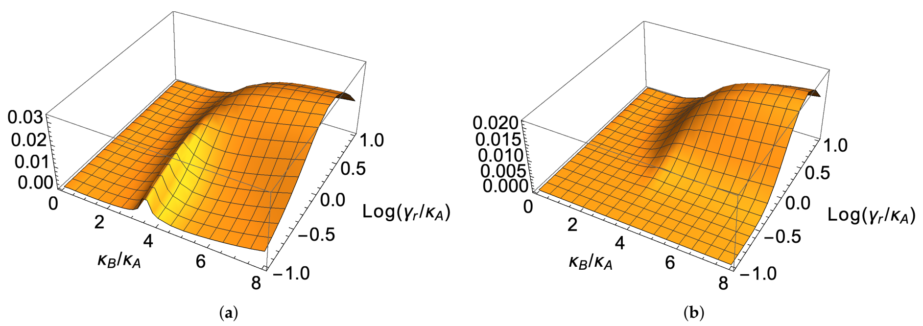
3.2. Simulations
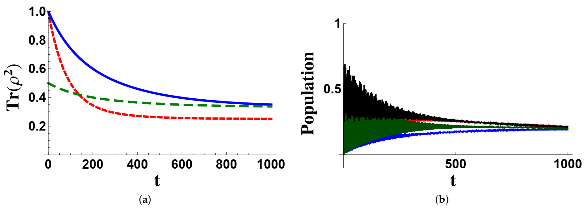
4. Dephasing
5. Discussion and Conclusions
Author Contributions
Funding
Data Availability Statement
Conflicts of Interest
References
- Acebrón, J.A.; Bonilla, L.L.; Vicente, C.J.P.; Ritort, F.; Spigler, R. The Kuramoto model: A simple paradigm for synchronization phenomena. Rev. Mod. Phys. 2005, 77, 137. [Google Scholar] [CrossRef] [Green Version]
- Pantaleone, J. Synchronization of metronomes. Am. J. Phys. 2002, 70, 992. [Google Scholar] [CrossRef]
- Maianti, M.; Pagliara, S.; Galimberti, G.; Parmigiani, F. Mechanics of two pendulums coupled by a stressed spring. Am. J. Phys. 2009, 77, 834–838. [Google Scholar] [CrossRef]
- Eckhardt, B.; Ott, E.; Strogatz, S.H.; Abrams, D.M.; McRobie, A. Modeling walker synchronization on the Millennium Bridge. Phys. Rev. E 2007, 75, 021110. [Google Scholar] [CrossRef]
- Angelini, L.; Lattanzi, G.; Maestri, R.; Marinazzo, D.; Nardulli, G.; Nitti, L.; Pellicoro, M.; Pinna, G.D.; Stramaglia, S. Phase shifts of synchronized oscillators and the systolic-diastolic blood pressure relation. Phys. Rev. E 2004, 69, 061923. [Google Scholar] [CrossRef] [Green Version]
- Giorgi, G.L.; Galve, F.; Manzano, G.; Colet, P.; Zambrini, R. Quantum correlations and mutual synchronization. Phys. Rev. A 2012, 85, 052101. [Google Scholar] [CrossRef] [Green Version]
- Manzano, G.; Galve, F.; Giorgi, G.L.; Harnández-Garcia, E.; Zambrini, R. Synchronization, quantum correlations and entanglement in oscillator networks. Sci. Rep. 2013, 3, 1439. [Google Scholar] [CrossRef] [Green Version]
- Militello, B.; Chruściński, D.; Napoli, A. Star network synchronization led by strong coupling-induced frequency squeezing. Phys. Scr. 2018, 93, 025201. [Google Scholar] [CrossRef] [Green Version]
- Bellomo, B.; Giorgi, G.L.; Palma, G.M.; Zambrini, R. Quantum synchronization as a local signature of super- and subradiance. Phys. Rev. A 2017, 95, 043807. [Google Scholar] [CrossRef] [Green Version]
- Cattaneo, M.; Giorgi, G.L.; Maniscalco, S.; Paraoanu, G.S.; Zambrini, R. Bath-Induced Collective Phenomena on Superconducting Qubits: Synchronization, Subradiance, and Entanglement Generation. Ann. Phys. 2021, 533, 2100038. [Google Scholar] [CrossRef]
- Huan, T.T.; Zhou, R.G.; Ian, H. Synchronization of two cavity-coupled qubits measured by entanglement. Sci. Rep. 2020, 10, 12975. [Google Scholar] [CrossRef]
- Arnesen, M.C.; Bose, S.; Vedral, V. Natural Thermal and Magnetic Entanglement in the 1D Heisenberg Model. Phys. Rev. Lett. 2001, 87, 017901. [Google Scholar] [CrossRef] [Green Version]
- Osterloh, A.; Amico, L.; Falci, G.; Fazio, R. Scaling of entanglement close to a quantum phase transition. Nature 2002, 416, 608. [Google Scholar] [CrossRef] [Green Version]
- Anzà, F.; Militello, B.; Messina, A. Tripartite thermal correlations in an inhomogeneous spin-star system. J. Phys. B At. Mol. Opt. Phys. 2010, 43, 205501. [Google Scholar] [CrossRef]
- Militello, B.; Nakazato, H.; Napoli, A. Synchronizing quantum harmonic oscillators through two-level systems. Phys. Rev. A 2017, 96, 023862. [Google Scholar] [CrossRef] [Green Version]
- You, J.Q.; Nori, F. Atomic physics and quantum optics using superconducting circuits. Nature 2011, 474, 589. [Google Scholar] [CrossRef] [Green Version]
- Xiang, Z.L.; Ashhab, S.; You, J.Q.; Nori, F. Hybrid quantum circuits: Superconducting circuits interacting with other quantum systems. Rev. Mod. Phys. 2013, 85, 623. [Google Scholar] [CrossRef] [Green Version]
- Wallraff, A.; Schuster, D.I.; Blais, A.; Frunzio, L.; Huang, R.-S.; Majer, J.; Kumar, S.; Girvin, S.M.; Schoelkopf, R.J. Strong coupling of a single photon to a superconducting qubit using circuit quantum electrodynamics. Nature 2004, 43, 162–167. [Google Scholar] [CrossRef] [Green Version]
- Blais, A.; Gambetta, J.; Wallraff, A.; Schuster, D.I.; Girvin, S.M.; Devoret, M.H.; Schoelkopf, R.J. Quantum-information processing with circuit quantum electrodynamics. Phys. Rev. A 2007, 75, 032329. [Google Scholar] [CrossRef] [Green Version]
- Chow, J.M.; Córcoles, A.D.; Gambetta, J.M.; Rigetti, C.; Johnson, B.R.; Smolin, J.A.; Rozen, J.R.; Keefe, G.A.; Rothwell, M.B.; Ketchen, M.B.; et al. Simple All-Microwave Entangling Gate for Fixed-Frequency Superconducting Qubits. Phys. Rev. Lett. 2011, 107, 080502. [Google Scholar] [CrossRef]
- Chow, J.M.; Gambetta, J.M.; Corcoles, A.D.; Merkel, S.T.; Smolin, J.A.; Rigetti, C.; Poletto, S.; Keefe, G.A.; Rothwell, M.B.; Rozen, J.R. Universal Quantum Gate Set Approaching Fault-Tolerant Thresholds with Superconducting Qubits. Phys. Rev. Lett. 2012, 109, 060501. [Google Scholar] [CrossRef] [PubMed] [Green Version]
- Carlo, L.D.; Reed, M.D.; Sun, L.; Johnson, B.R.; Chow, J.M.; Gambetta, J.M.; Frunzio, L.; Girvin, S.M.; Devoret, M.H.; Schoelkopf, R.J. Preparation and measurement of three-qubit entanglement in a superconducting circuit. Nature 2010, 467, 574. [Google Scholar]
- Ansmann, M.; Wang, H.; Bialczak, R.C.; Hofheinz, M.; Lucero, E.; Neeley, M.; O’Connell, A.D.; Sank, D.; Weides, M.; Wenner, J.; et al. Violation of Bell’s inequality in Josephson phase qubits. Nature 2009, 461, 504. [Google Scholar] [CrossRef] [PubMed]
- Pekola, J. Towards quantum thermodynamics in electronic circuits. Nat. Phys. 2015, 11, 118–123. [Google Scholar] [CrossRef] [Green Version]
- Cherubim, C.; Brito, F.; Deffner, S. Non-Thermal Quantum Engine in Transmon Qubits. Entropy 2019, 21, 545. [Google Scholar] [CrossRef] [Green Version]
- Pekola, J.P.; Khaymovich, I.M. Thermodynamics in Single-Electron Circuits and Superconducting Qubits. Annu. Rev. Condens. Matter Phys. 2019, 10, 193. [Google Scholar] [CrossRef]
- Elouard, C.; Thomas, G.; Maillet, O.; Pekola, J.P.; Jordan, A.N. Quantifying the quantum heat contribution from a driven superconducting circuit. Phys. Rev. E 2020, 102, 030102. [Google Scholar] [CrossRef]
- Rigetti, C.; Gambetta, J.M.; Poletto, S.; Plourde, B.L.T.; Chow, J.M.; Corcoles, A.D.; Smolin, J.A.; Merkel, S.T.; Rozen, J.R.; Keefe, G.A.; et al. Superconducting qubit in a waveguide cavity with a coherence time approaching 0.1 ms. Phys. Rev. B 2012, 86, 100506. [Google Scholar] [CrossRef] [Green Version]
- Lu, Y.; Bengtsson, A.; Burnett, J.J.; Wieg, E.; Suri, B.; Krantz, P.; Roudsari, A.F.; Kockum, A.F.; Gasparinetti, S.; Johansson, G.; et al. Characterizing decoherence rates of a superconducting qubit by direct microwave scattering. NPJ Quantum Inf. 2021, 7, 35. [Google Scholar] [CrossRef]
- Sevriuk, V.A.; Tan, K.Y.; Hyyppä, E.; Silveri, M.; Partanen, M.; Jenei, M.; Masuda, S.; Goetz, J.; Vesterinen, V.; Grönberg, L.; et al. Fast control of dissipation in a superconducting resonator. Appl. Phys. Lett. 2019, 115, 082601. [Google Scholar] [CrossRef]
- Jones, P.J.; Huhtamäki, J.A.M.; Salmilehto, J.; Tan, K.Y.; Möttxoxnen, M. Tunable electromagnetic environment for superconducting quantum bits. Sci. Rep. 2013, 3, 1987. [Google Scholar] [CrossRef] [Green Version]
- Scala, M.; Militello, B.; Messina, A.; Piilo, J.; Maniscalco, S. Microscopic derivation of the Jaynes-Cummings model with cavity losses. Phys. Rev. A 2007, 75, 013811. [Google Scholar] [CrossRef] [Green Version]
- Beaudoin, F.; Coish, W.A. Microscopic models for charge-noise-induced dephasing of solid-state qubits. Phys. Rev. B 2015, 91, 165432. [Google Scholar] [CrossRef] [Green Version]
- Scala, M.; Militello, B.; Messina, A.; Vitanov, N.V. Stimulated Raman adiabatic passage in an open quantum system: Master equation approach. Phys. Rev. A 2010, 81, 053847. [Google Scholar] [CrossRef] [Green Version]
- Scala, M.; Militello, B.; Messina, A.; Vitanov, N.V. Detuning effects in STIRAP processes in the presence of quantum noise. Opt. Spectrosc. 2011, 111, 589. [Google Scholar] [CrossRef]
- Zanardi, P.; Rasetti, M. Noiseless Quantum Codes. Phys. Rev. Lett. 1997, 79, 3306. [Google Scholar] [CrossRef] [Green Version]
- Zanardi, P.; Rossi, F. Quantum Information in Semiconductors: Noiseless Encoding in a Quantum-Dot Array. Phys. Rev. Lett. 1998, 81, 4752. [Google Scholar] [CrossRef] [Green Version]
- Chruscinski, D.; Messina, A.; Militello, B.; Napoli, A. Interaction-free evolution in the presence of time-dependent Hamiltonians. Phys. Rev. A 2015, 91, 042123. [Google Scholar] [CrossRef] [Green Version]
- Militello, B.; Chruscinski, D.; Messina, A.; Nalezyty, P.; Napoli, A. Generalized interaction-free evolutions. Phys. Rev. A 2016, 96, 022113. [Google Scholar] [CrossRef] [Green Version]


Publisher’s Note: MDPI stays neutral with regard to jurisdictional claims in published maps and institutional affiliations. |
© 2021 by the authors. Licensee MDPI, Basel, Switzerland. This article is an open access article distributed under the terms and conditions of the Creative Commons Attribution (CC BY) license (https://creativecommons.org/licenses/by/4.0/).
Share and Cite
Militello, B.; Napoli, A. Synchronizing Two Superconducting Qubits through a Dissipating Resonator. Entropy 2021, 23, 998. https://doi.org/10.3390/e23080998
Militello B, Napoli A. Synchronizing Two Superconducting Qubits through a Dissipating Resonator. Entropy. 2021; 23(8):998. https://doi.org/10.3390/e23080998
Chicago/Turabian StyleMilitello, Benedetto, and Anna Napoli. 2021. "Synchronizing Two Superconducting Qubits through a Dissipating Resonator" Entropy 23, no. 8: 998. https://doi.org/10.3390/e23080998