
Information Bottleneck Analysis by a Conditional Mutual Information Bound


Abstract
:1. Introduction
2. Related Work
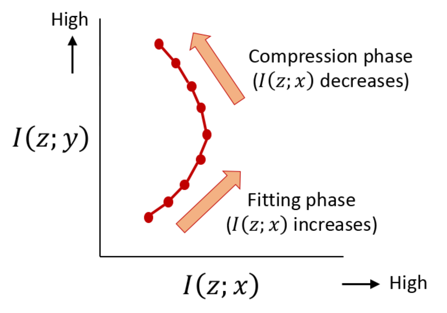
2.1. Information Bottleneck Theory
2.2. Task-Nuisance Decomposition
2.3. Non-Parametric Estimation of Mutual Information
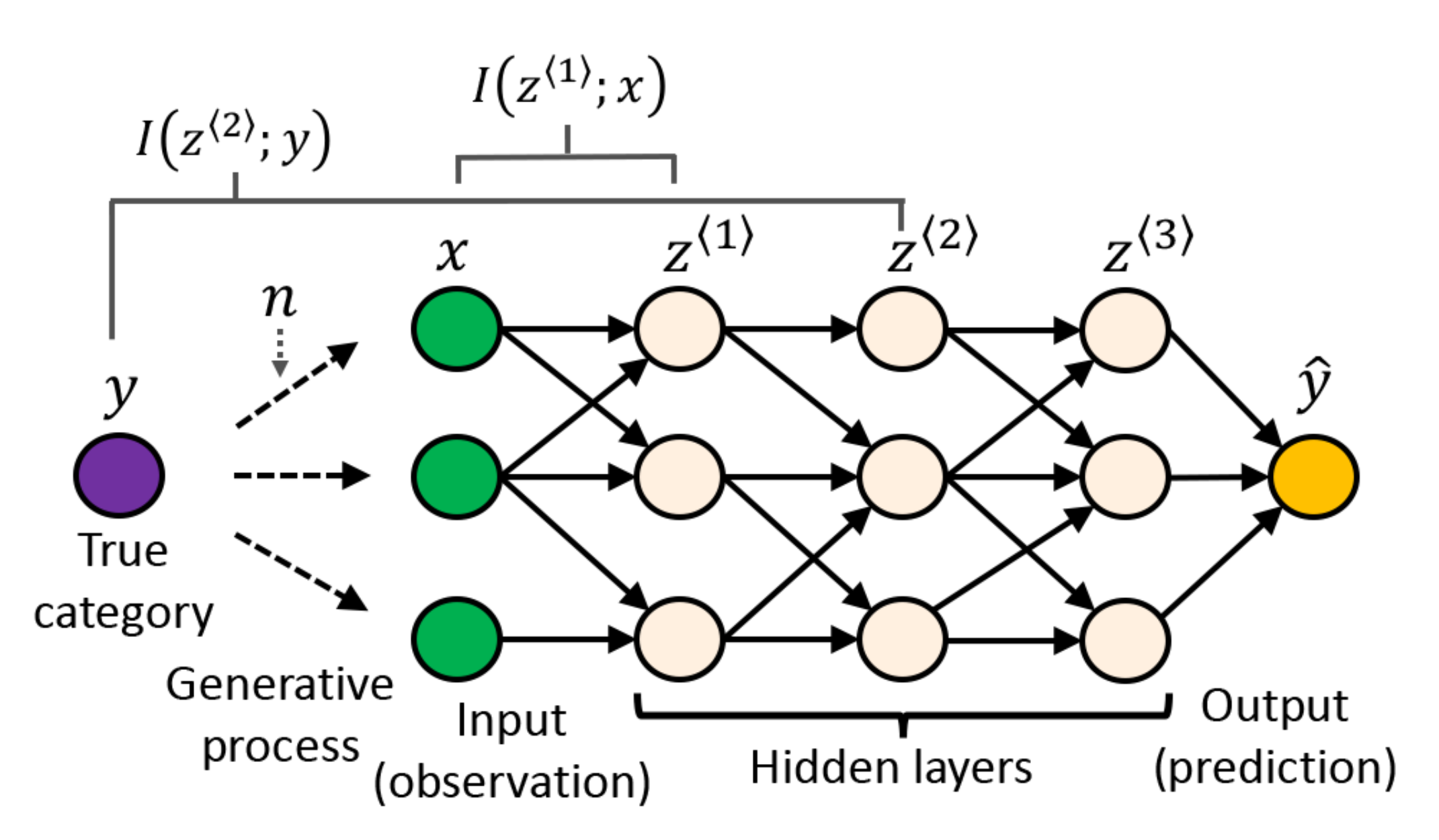
3. Method
3.1. Notations
3.2. Mathematical Property
3.3. Estimation
3.3.1. Conditional MINE (CMINE)
3.3.2. Averaged MINE (AMINE)
4. Implementation
4.1. Dataset, Architecture, and Parameters
4.2. Preprocessing before Estimation by MINE
4.3. Cluttering
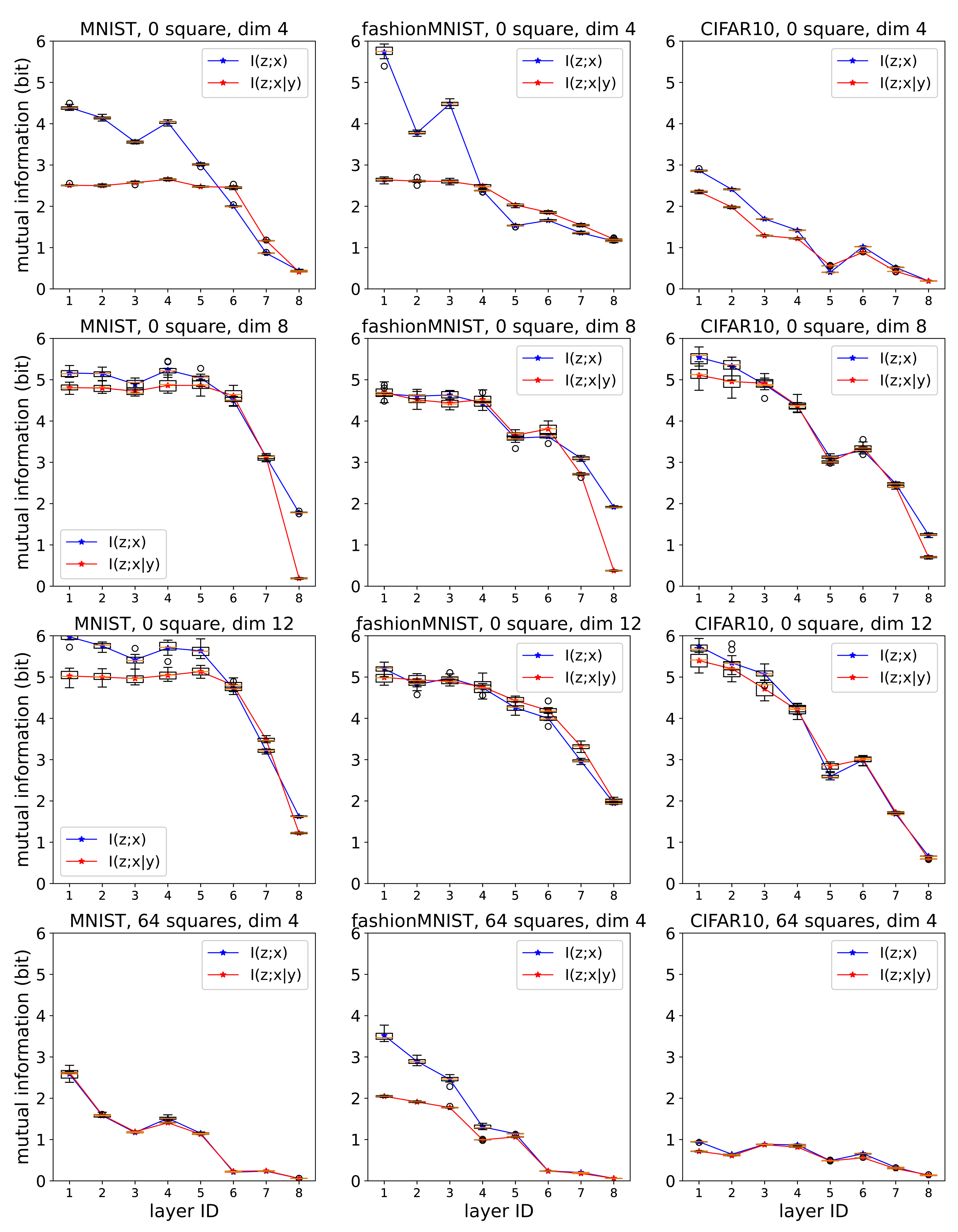
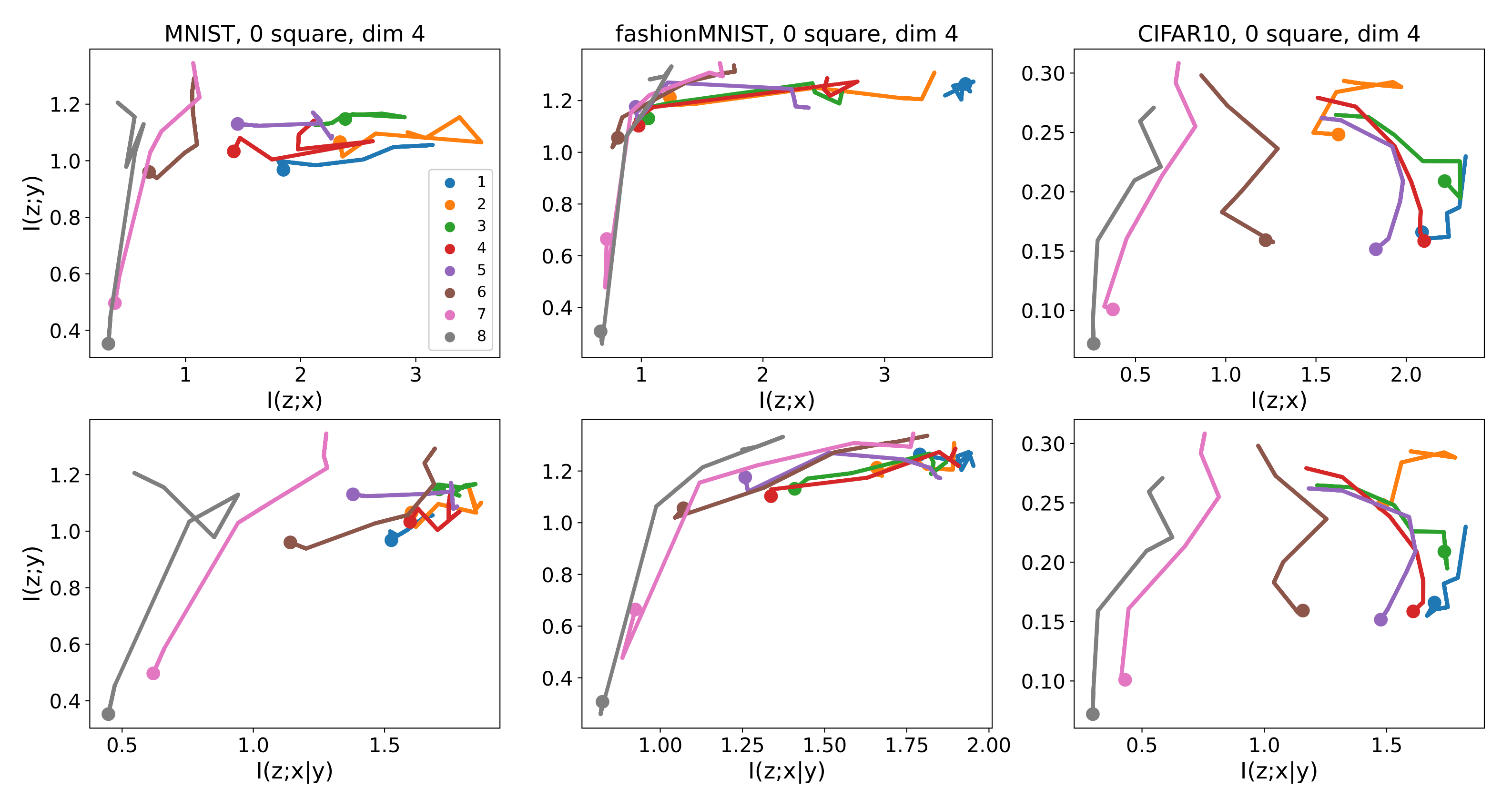
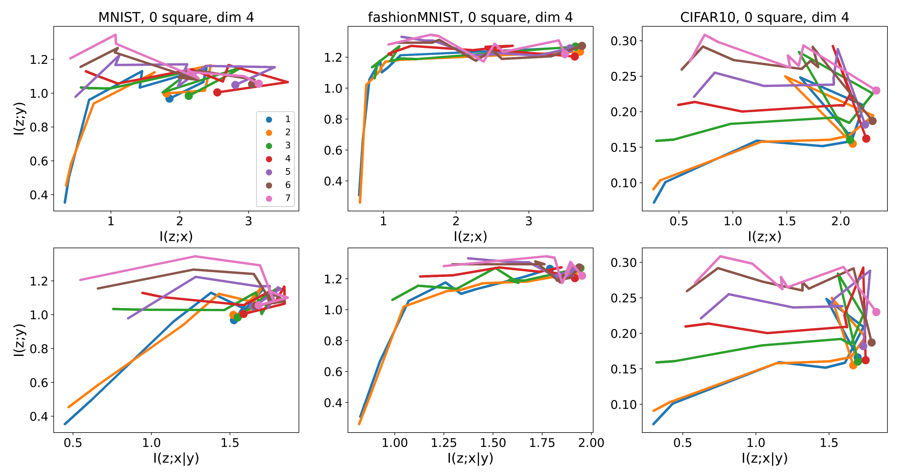
5. Experiments
5.1. Comparison of and across Layers
5.2. Information Planes
6. Conclusions
Author Contributions
Funding
Institutional Review Board Statement
Informed Consent Statement
Data Availability Statement
Conflicts of Interest
References
- Achille, A.; Soatto, S. Information dropout: Learning optimal representations through noisy computation. IEEE Trans. Pattern Anal. Mach. Intell. 2018, 40, 2897–2905. [Google Scholar] [CrossRef] [PubMed] [Green Version]
- Gabrié, M.; Manoel, A.; Luneau, C.; Barbier, J.; Macris, N.; Krzakala, F.; Zdeborová, L. Entropy and mutual information in models of deep neural networks. In Advances in Neural Information Processing Systems; The MIT Press: Cambridge, MA, USA, 2018; Volume 31. [Google Scholar]
- Hjelm, R.D.; Fedorov, A.; Lavoie-Marchildon, S.; Grewal, K.; Bachman, P.; Trischler, A.; Bengio, Y. Learning deep representations by mutual information estimation and maximization. In Proceedings of the 2019 International Conference on Learning Representations, New Orleans, LA, USA, 6–9 May 2019. [Google Scholar]
- Alemi, A.A.; Fischer, I.; Dillon, J.V.; Murphy, K. Deep Variational Information Bottleneck. In Proceedings of the 2019 International Conference on Learning Representations, New Orleans, LA, USA, 6–9 May 2019. [Google Scholar]
- Yu, S.; Princípe, J.C. Understanding autoencoders with information theoretic concepts. Neural Netw. 2019, 117, 104–123. [Google Scholar] [CrossRef] [PubMed] [Green Version]
- Yu, S.; Wickstrøm, K.; Jenssen, R.; Princípe, J.C. Understanding convolutional neural networks with information theory: An initial exploration. IEEE Trans. Neural Netw. Learn. Syst. 2021, 32, 435–442. [Google Scholar] [CrossRef]
- Tishby, N.; Pereira, F.C.; Bialek, W. The information bottleneck method. In Proceedings of the 37th annual Allerton Conference on Communication, Control, and Computing, Monticello, IL, USA, 22–24 September 1999; pp. 368–377. [Google Scholar]
- Achille, A.; Soatto, S. Emergence of Invariance and Disentanglement in Deep Representations. J. Mach. Learn. Res. 2018, 18, 1–34. [Google Scholar]
- Slonim, N.; Tishby, N. Agglomerative information bottleneck. In Proceedings of the 12th International Conference on Neural Information Processing Systems, Denver, CO, USA, 29 November–4 December 1999; pp. 617–623. [Google Scholar]
- Chechik, G.; Globerson, A.; Tishby, N.; Weiss, Y. Information Bottleneck for Gaussian Variables. J. Mach. Learn. Res. 2005, 6, 165–188. [Google Scholar]
- Harremoës, P.; Tishby, N. The information bottleneck revisited or how to choose a good distortion measure. In Proceedings of the 2007 IEEE International Symposium on Information Theory, Nice, France, 24–29 June 2007. [Google Scholar]
- Shamir, O.; Sabato, S.; Tishby, N. Learning and generalization with the information bottleneck. Theor. Comput. Sci. 2010, 411, 2696–2711. [Google Scholar] [CrossRef] [Green Version]
- Tishby, N.; Zaslavsky, N. Deep learning and the information bottleneck principle. In Proceedings of the IEEE Information Theory Workshop (ITW), Jeju Island, Korea, 11–15 October 2015; pp. 1–5. [Google Scholar]
- Schwartz-Ziv, R.; Tishby, N. Opening the black box of deep neural networks via information. arXiv 2017, arXiv:1703.00810. [Google Scholar]
- Balda, E.R.; Behboodi, A.; Mathar, R. On the Trajectory of Stochastic Gradient Descent in the Information Plane. arXiv 2018, arXiv:1807.08140. [Google Scholar]
- Goldfeld, Z.; van den Berg, E.; Greenewald, K.; Melnyk, I.; Nguyen, N.; Kingsbury, B.; Polyanskiy, Y. Estimating Information Flow in Deep Neural Networks. arXiv 2018, arXiv:1810.05728. [Google Scholar]
- Chelombiev, I.; Houghton, C.; O’Donnell, C. Adaptive estimators show information compression in deep neural networks. Proceedings of the 2019 International Conference on Learning Representations, New Orleans, LA, USA, 6–9 May 2019. [Google Scholar]
- Achille, A.; Paolini, G.; Soatto, S. Where is the Information in a Deep Neural Network? arXiv 2019, arXiv:1905.12213. [Google Scholar]
- Darlow, L.N.; Storkey, A. What Information Does a ResNet Compress? arXiv 2020, arXiv:2003.06254. [Google Scholar]
- Geiger, B.C. On Information Plane Analyses of Neural Network Classifiers—A Review. arXiv 2020, arXiv:2003.09671. [Google Scholar]
- Wieczorek, A.; Roth, V. On the Difference between the Information Bottleneck and the Deep Information Bottleneck. Entropy 2020, 22, 131. [Google Scholar] [CrossRef] [Green Version]
- Goldfeld, Z.; Polyanskiy, Y. The Information Bottleneck Problem and Its Applications in Machine Learning. arXiv 2020, arXiv:2004.14941. [Google Scholar] [CrossRef]
- Amjad, R.A.; Geiger, B.C. Learning Representations for Neural Network-Based Classification Using the Information Bottleneck Principle. IEEE Trans. Pattern Anal. Mach. Intell. 2020, 42, 2225–2239. [Google Scholar] [CrossRef] [PubMed] [Green Version]
- Fischer, I. The conditional entropy bottleneck. Entropy 2020, 22, 999. [Google Scholar] [CrossRef] [PubMed]
- Geiger, B.C.; Fischer, I.S. A comparison of variational bounds for the information bottleneck functional. Entropy 2020, 22, 1229. [Google Scholar] [CrossRef] [PubMed]
- Yu, X.; Yu, S.; Princípe, J.C. Deep Deterministic Information Bottleneck with Matrix-Based Entropy Functional. In Proceedings of the 2021 IEEE International Conference on Acoustics, Speech and Signal Processing (ICASSP), Toronto, ON, Canada, 6–11 June 2021. [Google Scholar]
- Giraldo, L.G.S.; Rao, M.; Princípe, J.C. Measures of entropy from data using infinitely divisible kernels. IEEE Trans. Inf. Theory 2014, 61, 535–548. [Google Scholar] [CrossRef] [Green Version]
- Yu, S.; Giraldo, L.G.S.; Jenssen, R.; Princípe, J.C. Multivariate extension of matrix-based Renyi’s α-order entropy functional. IEEE Trans. Pattern Anal. Mach. Intell. 2019, 42, 2960–2966. [Google Scholar] [CrossRef] [PubMed]
- Kraskov, A.; Stoegbauer, H.; Grassberger, P. Estimating Mutual Information. Phys. Rev. E 2004, 69, 066138. [Google Scholar] [CrossRef] [Green Version]
- Kandasamy, K.; Krishnamurthy, A.; Póczos, B.; Wasserman, L.; Robins, J.M. Nonparametric von Mises estimators for entropies, divergences and mutual informations. In Advances in Neural Information Processing Systems; The MIT Press: Cambridge, MA, USA, 2015; pp. 397–405. [Google Scholar]
- Belghazi, M.I.; Baratin, A.; Rajeswar, S.; Ozair, S.; Bengio, Y.; Courville, A.; Hjelm, R.D. Mutual information neural estimation. In Proceedings of the 35th International Conference on Machine Learning, Stockholm, Sweden, 10–15 July 2018; Volume 80, pp. 531–540. [Google Scholar]
- Elad, A.; Haviv, D.; Blau, Y.; Michaeli, T. Direct Validation of the Information Bottleneck Principle for Deep Nets. In Proceedings of the 2019 International Conference on Computer Vision Workshops, Seoul, Korea, 27–28 October 2019. [Google Scholar]
- Jónsson, H.; Cherubini, G.; Eleftheriou, E. Convergence of DNNs with mutual-information-based regularization. Entropy 2019, 22, 727. [Google Scholar] [CrossRef] [PubMed]
- Willems, F.M.J.; van der Meulen, E.C. The discrete memoryless multiple-access channel with cribbing encoders. IEEE Trans. Inf. Theory 1985, 31, 313–327. [Google Scholar] [CrossRef]
- Cover, T.M.; Thomas, J.A. Elements of Information Theory, 2nd ed.; Wiley-Interscience: Hoboken, NJ, USA, 2006. [Google Scholar]
- Moyer, D.; Gao, S.; Brekelmans, R.; Steeg, G.V.; Galstyan, A. Invariant representations without adversarial training. In Proceedings of the 32nd International Conference on Neural Information Processing Systems, Montreal, QC, Canada, 3–8 December 2018. [Google Scholar]
- Moon, K.R.; Sricharan, K., III; Hero, A.O. Ensemble estimation of mutual information. In Proceedings of the 2017 IEEE International Symposium on Information Theory, Aachen, Germany, 25–30 June 2017.
- Noshad, M.; Zeng, Y.; Hero, A.O. Scalable mutual information estimation using dependence graphs. In Proceedings of the 2019 IEEE International Conference on Acoustics, Speech and Signal Processing, Brighton, UK, 12–17 May 2019. [Google Scholar]
- Singh, S.; Póczos, B. Exponential concentration of a density functional estimator. In Advances in Neural Information Processing Systems; The MIT Press: Cambridge, MA, USA, 2014; pp. 3032–3040. [Google Scholar]


| Target network | Conv(3,3,8;1) - Conv(3,3,8;1) - Conv(3,3,8;1) - Conv(3,3,8;1) - Conv(3,3,8;4) - FC(100) - FC(16) - Softmax(10) |
| MINE network | FC(dim(a)) - FC(100) - FC(100) - FC(100) - FC(1) |
| Optim. | Learn. Rate | # of Samples | Batch Size | Epochs | |
|---|---|---|---|---|---|
| Target | Adam | 0.001 | 10,000 | 64 | 100 |
| MINE | Adam | 0.001 | 50,000 | 32 | 30 |
Publisher’s Note: MDPI stays neutral with regard to jurisdictional claims in published maps and institutional affiliations. |
© 2021 by the authors. Licensee MDPI, Basel, Switzerland. This article is an open access article distributed under the terms and conditions of the Creative Commons Attribution (CC BY) license (https://creativecommons.org/licenses/by/4.0/).
Share and Cite
Tezuka, T.; Namekawa, S. Information Bottleneck Analysis by a Conditional Mutual Information Bound. Entropy 2021, 23, 974. https://doi.org/10.3390/e23080974
Tezuka T, Namekawa S. Information Bottleneck Analysis by a Conditional Mutual Information Bound. Entropy. 2021; 23(8):974. https://doi.org/10.3390/e23080974
Chicago/Turabian StyleTezuka, Taro, and Shizuma Namekawa. 2021. "Information Bottleneck Analysis by a Conditional Mutual Information Bound" Entropy 23, no. 8: 974. https://doi.org/10.3390/e23080974