
The Renewed Role of Sweep Functions in Noisy Shortcuts to Adiabaticity


Abstract
:1. Introduction
2. Theoretical Background
2.1. Adiabatic Sweep Functions
2.2. Counterdiabatic Driving (STA)
2.3. Lindblad Master Equation
3. Results
3.1. Two-Level Avoided Crossing
3.2. Two-Qubit Gate
4. Discussion and Conclusions
Author Contributions
Funding
Data Availability Statement
Acknowledgments
Conflicts of Interest
Abbreviations
| STA | shortcuts to adiabaticity |
| CD | counterdiabatic |
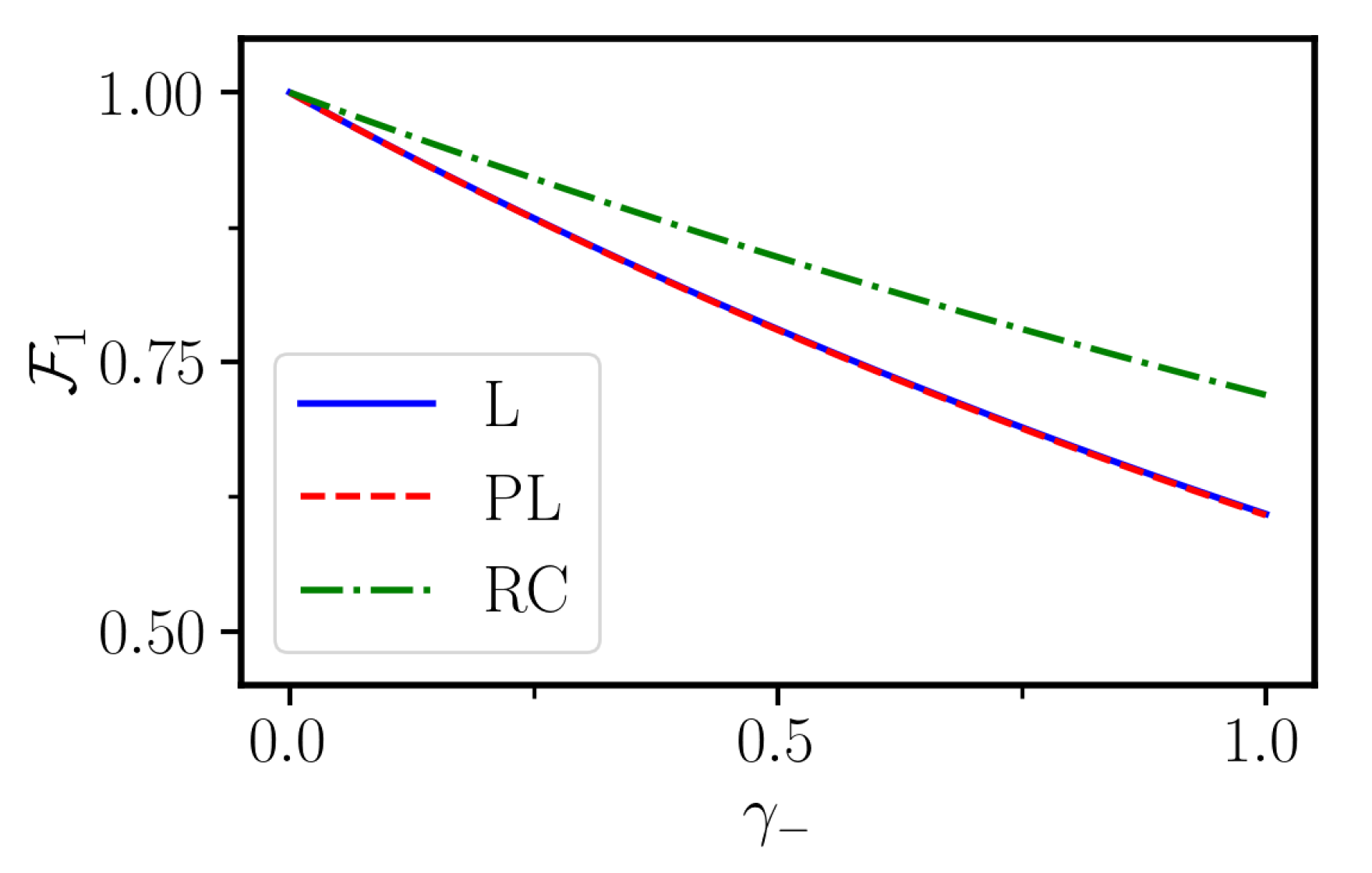
| L | linear |
| PL | polynomial |
| RC | Roland–Cerf |
Appendix A. Roland–Cerf Sweep Function
References
- Vitanov, N.V.; Rangelov, A.A.; Shore, B.W.; Bergmann, K. Stimulated Raman adiabatic passage in physics, chemistry, and beyond. Rev. Mod. Phys. 2017, 89, 015006. [Google Scholar] [CrossRef]
- Král, P.; Thanopulos, I.; Shapiro, M. Colloquium: Coherently controlled adiabatic passage. Rev. Mod. Phys. 2007, 79, 53–77. [Google Scholar] [CrossRef] [Green Version]
- Messiah, A. Quantum Mechanics; Dover Publications: New York, NY, USA, 1961. [Google Scholar]
- Rezakhani, A.T.; Kuo, W.J.; Hamma, A.; Lidar, D.A.; Zanardi, P. Quantum Adiabatic Brachistochrone. Phys. Rev. Lett. 2009, 103, 080502. [Google Scholar] [CrossRef] [PubMed] [Green Version]
- Lidar, D.A.; Rezakhani, A.T.; Hamma, A. Adiabatic approximation with exponential accuracy for many-body systems and quantum computation. J. Math. Phys. 2009, 50, 102106. [Google Scholar] [CrossRef] [Green Version]
- Albash, T.; Lidar, D.A. Decoherence in adiabatic quantum computation. Phys. Rev. A 2015, 91, 062320. [Google Scholar] [CrossRef] [Green Version]
- Mohseni, N.; Narozniak, M.; Pyrkov, A.N.; Ivannikov, V.; Dowling, J.P.; Byrnes, T. Error suppression in adiabatic quantum computing with qubit ensembles. NPJ Quantum Inf. 2021, 7, 71. [Google Scholar] [CrossRef]
- Guéry-Odelin, D.; Ruschhaupt, A.; Kiely, A.; Torrontegui, E.; Martínez-Garaot, S.; Muga, J.G. Shortcuts to adiabaticity: Concepts, methods, and applications. Rev. Mod. Phys. 2019, 91, 045001. [Google Scholar] [CrossRef]
- Torrontegui, E.; Ibáñez, S.; Martí nez-Garaot, S.; Modugno, M.; del Campo, A.; Guéry-Odelin, D.; Ruschhaupt, A.; Chen, X.; Muga, J.G. Shortcuts to Adiabaticity. Adv. At. Mol. Opt. Phys. 2013, 62, 117–169. [Google Scholar] [CrossRef] [Green Version]
- del Campo, A.; Kim, K. Focus on Shortcuts to Adiabaticity. New J. Phys. 2019, 21, 050201. [Google Scholar] [CrossRef]
- Ibáñez, S.; Chen, X.; Torrontegui, E.; Muga, J.G.; Ruschhaupt, A. Multiple Schrödinger Pictures and Dynamics in Shortcuts to Adiabaticity. Phys. Rev. Lett. 2012, 109, 100403. [Google Scholar] [CrossRef] [Green Version]
- del Campo, A. Shortcuts to Adiabaticity by Counterdiabatic Driving. Phys. Rev. Lett. 2013, 111, 100502. [Google Scholar] [CrossRef] [Green Version]
- Baksic, A.; Ribeiro, H.; Clerk, A.A. Speeding up Adiabatic Quantum State Transfer by Using Dressed States. Phys. Rev. Lett. 2016, 116, 230503. [Google Scholar] [CrossRef] [Green Version]
- Martínez-Garaot, S.; Torrontegui, E.; Chen, X.; Muga, J.G. Shortcuts to adiabaticity in three-level systems using Lie transforms. Phys. Rev. A 2014, 89, 053408. [Google Scholar] [CrossRef] [Green Version]
- Chen, X.; Torrontegui, E.; Muga, J.G. Lewis-Riesenfeld invariants and transitionless quantum driving. Phys. Rev. A 2011, 83, 062116. [Google Scholar] [CrossRef] [Green Version]
- Petiziol, F.; Dive, B.; Mintert, F.; Wimberger, S. Fast adiabatic evolution by oscillating initial Hamiltonians. Phys. Rev. A 2018, 98, 043436. [Google Scholar] [CrossRef] [Green Version]
- Sels, D.; Polkovnikov, A. Minimizing irreversible losses in quantum systems by local counterdiabatic driving. Proc. Natl. Acad. Sci. USA 2017, 114, E3909–E3916. [Google Scholar] [CrossRef] [PubMed] [Green Version]
- Opatrný, T.; Mølmer, K. Partial suppression of nonadiabatic transitions. New J. Phys. 2014, 16, 015025. [Google Scholar] [CrossRef] [Green Version]
- Chen, Y.H.; Xia, Y.; Wu, Q.C.; Huang, B.H.; Song, J. Method for constructing shortcuts to adiabaticity by a substitute of counterdiabatic driving terms. Phys. Rev. A 2016, 93, 052109. [Google Scholar] [CrossRef] [Green Version]
- Giannelli, L.; Arimondo, E. Three-level superadiabatic quantum driving. Phys. Rev. A 2014, 89, 033419. [Google Scholar] [CrossRef] [Green Version]
- Eckardt, A. Colloquium: Atomic quantum gases in periodically driven optical lattices. Rev. Mod. Phys. 2017, 89, 011004. [Google Scholar] [CrossRef] [Green Version]
- Decker, K.S.C.; Karrasch, C.; Eisert, J.; Kennes, D.M. Floquet Engineering Topological Many-Body Localized Systems. Phys. Rev. Lett. 2020, 124, 190601. [Google Scholar] [CrossRef] [PubMed]
- Claeys, P.W.; Pandey, M.; Sels, D.; Polkovnikov, A. Floquet-Engineering Counterdiabatic Protocols in Quantum Many-Body Systems. Phys. Rev. Lett. 2019, 123, 090602. [Google Scholar] [CrossRef] [Green Version]
- Sameti, M.; Hartmann, M.J. Floquet engineering in superconducting circuits: From arbitrary spin-spin interactions to the Kitaev honeycomb model. Phys. Rev. A 2019, 99, 012333. [Google Scholar] [CrossRef] [Green Version]
- Bukov, M.; D’Alessio, L.; Polkovnikov, A. Universal high-frequency behavior of periodically driven systems: From dynamical stabilization to Floquet engineering. Adv. Phys. 2015, 64, 139–226. [Google Scholar] [CrossRef] [Green Version]
- Boyers, E.; Pandey, M.; Campbell, D.K.; Polkovnikov, A.; Sels, D.; Sushkov, A.O. Floquet-engineered quantum state manipulation in a noisy qubit. Phys. Rev. A 2019, 100, 012341. [Google Scholar] [CrossRef] [Green Version]
- Villazon, T.; Claeys, P.W.; Polkovnikov, A.; Chandran, A. Shortcuts to dynamic polarization. Phys. Rev. B 2021, 103, 075118. [Google Scholar] [CrossRef]
- Bartels, B.; Mintert, F. Smooth optimal control with Floquet theory. Phys. Rev. A 2013, 88, 052315. [Google Scholar] [CrossRef] [Green Version]
- Lucas, F.; Mintert, F.; Buchleitner, A. Tailoring many-body entanglement through local control. Phys. Rev. A 2013, 88, 032306. [Google Scholar] [CrossRef] [Green Version]
- Zhou, B.B.; Baksic, A.; Ribeiro, H.; Yale, C.G.; Heremans, F.J.; Jerger, P.; Auer, A.; Burkard, G.; Clerk, A.A.; Awschalom, D.D. Accelerated quantum control using superadiabatic dynamics in a solid-state lambda system. Nat. Phys. 2017, 13, 330–334. [Google Scholar] [CrossRef] [Green Version]
- Masuda, S.; Rice, S.A. A model study of assisted adiabatic transfer of population in the presence of collisional dephasing. J. Chem. Phys. 2015, 142, 244303. [Google Scholar] [CrossRef] [PubMed]
- Levy, A.; Torrontegui, E.; Kosloff, R. Action-noise-assisted quantum control. Phys. Rev. A 2017, 96, 033417. [Google Scholar] [CrossRef] [Green Version]
- Levy, A.; Kiely, A.; Muga, J.G.; Kosloff, R.; Torrontegui, E. Noise resistant quantum control using dynamical invariants. New J. Phys. 2018, 20, 025006. [Google Scholar] [CrossRef]
- Roland, J.; Cerf, N.J. Quantum search by local adiabatic evolution. Phys. Rev. A 2002, 65, 042308. [Google Scholar] [CrossRef] [Green Version]
- Petiziol, F.; Dive, B.; Carretta, S.; Mannella, R.; Mintert, F.; Wimberger, S. Accelerating adiabatic protocols for entangling two qubits in circuit QED. Phys. Rev. A 2019, 99, 042315. [Google Scholar] [CrossRef] [Green Version]
- Berry, M.V. Transitionless quantum driving. J. Phys. A 2009, 42, 365303. [Google Scholar] [CrossRef] [Green Version]
- Demirplak, M.; Rice, S.A. Adiabatic Population Transfer with Control Fields. J. Phys. Chem. A 2003, 107, 9937–9945. [Google Scholar] [CrossRef]
- Breuer, H.P.; Petruccione, F. The Theory of Open Quantum Systems; Oxford University Press: Oxford, UK, 2007; p. 656. [Google Scholar] [CrossRef] [Green Version]
- Berry, M.V. Two-State Quantum Asymptotics. Ann. N. Y. Acad. Sci. 1995, 755, 303–317. [Google Scholar] [CrossRef]
- Walls, D.F.; Milburn, G.J. Quantum Optics; Springer: Berlin, Germany, 2008. [Google Scholar]
- Sompet, P.; Szigeti, S.S.; Schwartz, E.; Bradley, A.S.; Andersen, M.F. Thermally robust spin correlations between two 85Rb atoms in an optical microtrap. Nat. Commun. 2019, 10, 1889. [Google Scholar] [CrossRef] [PubMed]
- Reynolds, L.A.; Schwartz, E.; Ebling, U.; Weyland, M.; Brand, J.; Andersen, M.F. Direct Measurements of Collisional Dynamics in Cold Atom Triads. Phys. Rev. Lett. 2020, 124, 073401. [Google Scholar] [CrossRef] [Green Version]
- Weyland, M.; Szigeti, S.S.; Hobbs, R.A.B.; Ruksasakchai, P.; Sanchez, L.; Andersen, M.F. Pair Correlations and Photoassociation Dynamics of Two Atoms in an Optical Tweezer. Phys. Rev. Lett. 2021, 126, 083401. [Google Scholar] [CrossRef]
- Nielsen, M.A.; Chuang, I.L. Quantum Computation and Quantum Information; Cambridge University Press: Cambridge, UK, 2010. [Google Scholar] [CrossRef] [Green Version]
- Clerk, A.A.; Devoret, M.H.; Girvin, S.M.; Marquardt, F.; Schoelkopf, R.J. Introduction to quantum noise, measurement, and amplification. Rev. Mod. Phys. 2010, 82, 1155–1208. [Google Scholar] [CrossRef]
- Ralph, T.C.; Bartlett, S.D.; O’Brien, J.L.; Pryde, G.J.; Wiseman, H.M. Quantum nondemolition measurements for quantum information. Phys. Rev. A 2006, 73, 012113. [Google Scholar] [CrossRef] [Green Version]
- Zhang, C.; Pokorny, F.; Li, W.; Higgins, G.; Pöschl, A.; Lesanovsky, I.; Hennrich, M. Submicrosecond entangling gate between trapped ions via Rydberg interaction. Nature 2020, 580, 345–349. [Google Scholar] [CrossRef] [PubMed] [Green Version]
- Blais, A.; Grimsmo, A.L.; Girvin, S.M.; Wallraff, A. Circuit quantum electrodynamics. Rev. Mod. Phys. 2021, 93, 025005. [Google Scholar] [CrossRef]
- Damski, B.; Zurek, W.H. Adiabatic-impulse approximation for avoided level crossings: From phase-transition dynamics to Landau-Zener evolutions and back again. Phys. Rev. A 2006, 73, 063405. [Google Scholar] [CrossRef] [Green Version]
- Blais, A.; Huang, R.S.; Wallraff, A.; Girvin, S.M.; Schoelkopf, R.J. Cavity quantum electrodynamics for superconducting electrical circuits: An architecture for quantum computation. Phys. Rev. A 2004, 69, 062320. [Google Scholar] [CrossRef] [Green Version]
- Krantz, P.; Kjaergaard, M.; Yan, F.; Orlando, T.P.; Gustavsson, S.; Oliver, W.D. A quantum engineer’s guide to superconducting qubits. Appl. Phys. Rev. 2019, 6, 021318. [Google Scholar] [CrossRef]
- Gu, X.; Kockum, A.F.; Miranowicz, A.; Liu, Y.; Nori, F. Microwave photonics with superconducting quantum circuits. Phys. Rep. 2017, 718–719, 1–102. [Google Scholar] [CrossRef]
- Blais, A.; Gambetta, J.; Wallraff, A.; Schuster, D.I.; Girvin, S.M.; Devoret, M.H.; Schoelkopf, R.J. Quantum-information processing with circuit quantum electrodynamics. Phys. Rev. A 2007, 75, 032329. [Google Scholar] [CrossRef] [Green Version]
- Majer, J.; Chow, J.M.; Gambetta, J.M.; Koch, J.; Johnson, B.R.; Schreier, J.A.; Frunzio, L.; Schuster, D.I.; Houck, A.A.; Wallraff, A.; et al. Coupling superconducting qubits via a cavity bus. Nature 2007, 449, 443–447. [Google Scholar] [CrossRef] [PubMed] [Green Version]
- Bason, M.G.; Viteau, M.; Malossi, N.; Huillery, P.; Arimondo, E.; Ciampini, D.; Fazio, R.; Giovannetti, V.; Mannella, R.; Morsch, O. High-fidelity quantum driving. Nat. Phys. 2012, 8. [Google Scholar] [CrossRef] [Green Version]
- Amin, M.H.S. Consistency of the Adiabatic Theorem. Phys. Rev. Lett. 2009, 102, 220401. [Google Scholar] [CrossRef] [PubMed] [Green Version]


Publisher’s Note: MDPI stays neutral with regard to jurisdictional claims in published maps and institutional affiliations. |
© 2021 by the authors. Licensee MDPI, Basel, Switzerland. This article is an open access article distributed under the terms and conditions of the Creative Commons Attribution (CC BY) license (https://creativecommons.org/licenses/by/4.0/).
Share and Cite
Delvecchio, M.; Petiziol, F.; Wimberger, S. The Renewed Role of Sweep Functions in Noisy Shortcuts to Adiabaticity. Entropy 2021, 23, 897. https://doi.org/10.3390/e23070897
Delvecchio M, Petiziol F, Wimberger S. The Renewed Role of Sweep Functions in Noisy Shortcuts to Adiabaticity. Entropy. 2021; 23(7):897. https://doi.org/10.3390/e23070897
Chicago/Turabian StyleDelvecchio, Michele, Francesco Petiziol, and Sandro Wimberger. 2021. "The Renewed Role of Sweep Functions in Noisy Shortcuts to Adiabaticity" Entropy 23, no. 7: 897. https://doi.org/10.3390/e23070897