Dynamic Risk Measures for Processes via Backward Stochastic Differential Equations Associated with Lévy Processes

Abstract

In this paper, we study the dynamic risk measures for processes induced by backward stochastic differential equations driven by Teugel’s martingales associated with Lévy processes (BSDELs). The representation theorem for generators of BSDELs is provided. Furthermore, the time consistency of the coherent and convex dynamic risk measures for processes is characterized by means of the generators of BSDELs. Moreover, the coherency and convexity of dynamic risk measures for processes are characterized by the generators of BSDELs. Finally, we provide two numerical examples to illustrate the proposed dynamic risk measures.

1. Introduction

Let $(\Omega ,\mathcal{F},\mathrm{P})$ be a probability space and $T>0$ be a fixed terminal time. Let $\{B_t,0\le t<\infty \}$ and $\{L_t,0\le t<\infty \}$ be two mutually independent processes defined on $(\Omega ,\mathcal{F},\mathrm{P})$, where $\{B_t,0\le t<\infty \}$ is a one-dimensional Brownian motion and $\{L_t,0\le t<\infty \}$ is a $\mathcal{R}$-valued Lévy process corresponding to a standard Lévy measure $\nu$ satisfying the following conditions:

(i)

${\int }_{\mathcal{R}}(1\wedge y^2)\nu \left(dy\right)<\infty$,

(ii)

${\int }_{{(-\epsilon ,\epsilon )}^c}{e}^{\lambda \left|y\right|}\nu \left(dy\right)<\infty$, for some $\lambda >0$ and for every $\epsilon >0.$

Let $\mathbb{F}=\{{\mathcal{F}}_t,t\ge 0\}$ be the natural filtration generated by $\{B_t,0\le t<\infty \}$ and $\{L_t,0\le t<\infty \}$.

Throughout this paper, we consider the following integral equation:

$$\begin{array}{c}\hfill Y_t=\xi +{\int }_t^{T}g\left(s,Y_s,Z_s,K_s\right)ds-{\int }_t^T{Z}_{s}d{B}_s-\sum _{i=1}^{\infty }{\int }_t^T{K}_s^{\left(i\right)}d{H}_s^{\left(i\right)},t\in [0,T],\end{array}$$

(1)

where the terminal value $\xi$ is a given ${\mathcal{F}}_T$ -measurable square integrable random variable, $g(·)$ is a given map, and $H_t^{\left(i\right)}$ is the orthonormalized Teugel’s martingale of order i associated with the Lévy process $\{L_t,0\le t<\infty \}$. The above equation is called backward stochastic differential equations associated with Lévy processes (BSDELs) introduced by Bahlali et al. [1]. When Equation (1) is independent of Teugel’s martingales, then Equation (1) is reduced to the following form:

$$\begin{array}{c}\hfill Y_t=\xi +{\int }_t^{T}g\left(s,Y_s,Z_s,K_s\right)ds-{\int }_t^T{Z}_{s}d{B}_s,t\in [0,T],\end{array}$$

(2)

which is the classical backward stochastic differential equations (BSDEs) introduced by Pardoux and Peng [2] first. Pardoux and Peng [2] proved that there exists a unique adapted and square integrable solution of the BSDE (2) under uniform Lipschitz condition on g. BSDELs can be seen as a natural generalization of BSDEs. Nualart and Schoutens [3] provided a martingale representation theorem associated with Lévy processes. Furthermore, Nualart and Schoutens [4] extended the classical BSDEs to BSDELs and established the existence and uniqueness of solutions for the BSDEL (1) which is independent of Brownian motion. For more studies on BSDELs, see El Otmani [5,6], Ren et al. [7], Ren and El Otmani [8], and the references therein.

Briand et al. [9] first studied the representation theorem for generators of BSDEs under the continuous assumption on the generators with respect to t and $E\left[{sup}_{t\in [0,T]}\right|g(t,0,0){|}^2<\infty ]$. Jiang [10] obtained the representation theorem for Lipschitz generators of BSDEs. Zhang and Fan [11] provided a representation theorem for generators of BSDEs with infinite time intervals and linear growth generators. For more studies on the representation theorem for generators of BSDEs, we refer to Song et al. [12], Xiao and Fan [13], Zheng and Li [14], Wu and Zhang [15], and the references therein. In this paper, we are concerned with representation theorem for generators of the BSDELs (1). For this issue, to our best knowledge, there is no reference available in the literature.

Risk measures have been extensively researched in finance and in the insurance industry such as the adjustment of life insurance rates. To quantify the riskiness of financial positions, Artzner et al. [16,17] introduced the concept of coherent risk measure by proposing the theory of axiomatic system of capital requirements. By weakening coherence axioms, Föllmer and Schied [18] and, independently, Frittelli and Rosazza Gianin [19] introduced convex risk measures. Their work attracts many researcher’s interest. For example, see Delbaen [20], Cheridito et al. [21,22], Riedel [23], Rosazza Gianin [24], Detlefsen and Scandolo [25], Klöppel and Schweizer [26], Delbaen et al. [27], Acciaio et al. [28], Föllmer and Schied [29], Song et al. [30], and the references therein.

BSDEs have become a popular tool for studying dynamic risk measures since Peng [31] investigated BSDEs and g-expectations. For instance, El Karoui et al. [32] studied dynamic risk measures for random variables via BSDEs. Jiang [33] established the one-to-one relationship between the generators BSDEs and the corresponding dynamic risk measures for random variables. Penner and Réveillac [34] established a link between risk measures for processes and BSDEs and studied the corresponding time-consistent dynamic risk measures for processes induced by BSDEs. Xu [35] studied multidimensional dynamic convex risk measures induced by conditional g-expectations. Ji et al. [36] provided some time-consistent dynamic risk measures for processes via BSDEs, and established the one-to-one relationship between the generators BSDEs and the corresponding dynamic risk measures for processes. A essential property for dynamic risk measures is time-consistency (see Bion-Nadal [37,38]). These time-consistent dynamic risk measures are constructed by BSDEs where the financial positions are random variables at some terminal time. However, time-inconsistent preference is realistic in financial markets. For example, see Yong [39], Wang and Shi [40], and Agram [41].

In this paper, we study dynamic risk measures induced by BSDELs. In a financial market, jump dynamics, which might be caused by policy interference, natural accidents, and so on, indeed exist. For instance, a stock’s price and its return show abnormal and sharp volatility. Thus, investors can be risk-averse and master the best time of those jump dynamics if they have sufficient awareness. Therefore, the processes of stock price and its return can be modeled by BSDELs (1). Based on the above consideration, we construct dynamic risk measures by means of BSDELs (1). First, the representation theorem for generators of BSDELs is provided. Second, the time-consistency of the coherent and convex dynamic risk measures for processes is characterized by means of the generators of BSDELs. Moreover, the coherency and convexity of dynamic risk measures for processes are characterized by the generators of BSDELs. Finally, we provide two numerical examples to illustrate the proposed dynamic risk measures. The obtained results extends the results of Briand et al. [9], Jiang [10], Penner and Réveillac [34], and Ji et al. [36].

The rest of the paper is organized as follows. In Section 2, we briefly state some preliminaries including the definitions of time-consistent dynamic convex and coherent risk measures for processes and some results on BSDELs. The definition of dynamic risk measures for processes induced by BSDELs is also provided in Section 2. In Section 3, our main results are presented, that is, the coherency and convexity of dynamic risk measures for processes are characterized by the generators of BSDELs, and the representation theorem for generators of BSDELs is provided. Section 4 contains all the proofs of the main results of this paper. We provide two numerical examples to illustrate the proposed dynamic risk measures in Section 5. Finally, conclusions are summarized.

2. Preliminaries

2.1. Notations of Dynamic Risk Measures for Processes

For any positive integer n and $z\in {\mathcal{R}}^n$, $\left|z\right|$ denotes its Euclidean norm. For any $t\in [0,T]$, we introduce the following spaces.

• L${}^2(\Omega ,{\mathcal{F}}_t,\mathrm{P})$ is the space of random variables $\xi$ which are ${\mathcal{F}}_t$-measurable with $E\left[\right|\xi {|}^2]<\infty$.
• L${}^{\infty }(\Omega ,{\mathcal{F}}_t,\mathrm{P})$ is the space of random variables $\xi$ which are ${\mathcal{F}}_t$-measurable and essentially bounded.
• ${\mathcal{H}}_T^2$ is the space of (${\mathcal{F}}_t$)-progressively measurable processes $Z:\Omega \times [0,T]\to \mathcal{R}$ such that

  $${∥Z∥}_{{\mathcal{H}}_T^2}^2=E\left[{\int }_0^T{\left|Z_s\right|}^{2}ds\right]<\infty .$$
• ${\mathcal{S}}_T^2$ is the space of (${\mathcal{F}}_t$)-progressively measurable and càdlàg processes $Y:\Omega \times [0,T]\to \mathcal{R}$ such that

  $${∥Y∥}_{{\mathcal{S}}_T^2}^2=E\left[\underset{t\in [0,T]}{sup}{\left|Y_t\right|}^2\right]<\infty .$$
• ${\mathcal{R}}^{\infty }$ is the space of (${\mathcal{F}}_t$)-progressively measurable and càdlàg processes $\phi :\Omega \times [0,T]\to \mathcal{R}$ such that

  $${∥\phi ∥}_{{\mathcal{R}}^{\infty }}={∥\underset{t\in [0,T]}{sup}\left|{\phi }_t\right|∥}_{\infty }<\infty .$$
• ${\ell }^2$ is the space of real valued sequences ${\left(x_n\right)}_{n\ge 0}$ such that

  $${\parallel x\parallel }_{{\ell }^2}^2=\sum _{n=1}^{\infty }{\left|x_n\right|}^2<\infty .$$
• ${\mathcal{P}}^2\left({\ell }^2\right)$ is the space of predictable processes K taking values in ${\ell }^2$ such that

  $${\parallel K\parallel }_{{\mathcal{P}}^2\left({\ell }^2\right)}^2=E\left[{\int }_0^T{\parallel K_s\parallel }_{{\ell }^2}^{2}ds\right]=\sum _{i=1}^{\infty }E\left[{\int }_0^T{\left|K_s^{\left(i\right)}\right|}^{2}ds\right]<\infty .$$
• ${\mathcal{E}}^2$ is the Banach space of processes $(Y,Z,K)\in {\mathcal{S}}_T^2\times H_T^2\times {\mathcal{P}}^2\left({\ell }^2\right)$ under the following norm

  $${∥(Y,Z,K)∥}_{{\mathcal{E}}^2}^2=E\left[\underset{t\in [0,T]}{sup}|Y_t{|}^2+{\int }_0^T|Z_s{|}^{2}ds+{\int }_0^T{\parallel K_s\parallel }_{{\ell }^2}^{2}ds\right].$$

For the convenience of the reader, we introduce the concept of related time-consistent dynamic risk measures for processes, see Cheridito et al. [22], Penner and Réveillac [34], and Ji et al. [36].

For $0\le t\le s\le T$, we define the projection ${\pi }_{t,s}:={\mathcal{R}}^{\infty }\to {\mathcal{R}}^{\infty }$ as

$${\pi }_{t,s}{\left(X\right)}_r=1_{[t,T]}\left(r\right)X_{r\wedge s},r\in [0,T],$$

$${\mathcal{R}}_{t,s}^{\infty }:={\pi }_{t,s}\left({\mathcal{R}}^{\infty }\right)and{\mathcal{R}}_t^{\infty }:={\pi }_{t,T}\left({\mathcal{R}}^{\infty }\right).$$

On a general level, a conditional risk measure ${\rho }_t$ is any map from ${\mathcal{R}}_t^{\infty }$ to $L^{\infty }(\Omega ,{\mathcal{F}}_t,\mathrm{P})$. ${\rho }_t$ can be described as a risk assessment at time t, which is taken into account the information available up to this time. For $t\in [0,T]$, the map ${\rho }_t$ has the following usual axioms for all $X,Y\in {\mathcal{R}}_t^{\infty }$.

(A)

(Conditional cash invariance) For all $m\in L^{\infty }(\Omega ,{\mathcal{F}}_t,\mathrm{P})$,

$${\rho }_t(X+m{1}_{[t,T]})={\rho }_t\left(X\right)-m.$$

(B)

(Monotonicity) ${\rho }_t\left(X\right)\ge {\rho }_t\left(Y\right),\mathrm{if}X\le Y.$

(C)

(Subadditivity) ${\rho }_t(X+Y)\le {\rho }_t(X+Y).$

(D)

(Conditional positive homogeneity) ${\rho }_t\left(\lambda X\right)=\lambda {\rho }_t\left(X\right),\forall \lambda \in L^{\infty }(\Omega ,{\mathcal{F}}_t,\mathrm{P}),\lambda \ge 0.$

(E)

(Conditional convexity) For all $\lambda \in L^{\infty }(\Omega ,{\mathcal{F}}_t,\mathrm{P})$, $\lambda \in [0,1]$,

$${\rho }_t\left(\lambda X+(1-\lambda )Y\right)\le \lambda {\rho }_t\left(X\right)+(1-\lambda ){\rho }_t\left(Y\right).$$

(F)

(Normalization) ${\rho }_t\left(0\right)=0.$

Definition 1.

A map ${\rho }_t:{\mathcal{R}}_t^{\infty }\to L^{\infty }(\Omega ,{\mathcal{F}}_t,\mathrm{P})$ for $t\in [0,T]$ is called a conditional coherent risk measure for processes, if it satisfies (A), (B), (C), and (D).

Definition 2.

A map ${\rho }_t:{\mathcal{R}}_t^{\infty }\to L^{\infty }(\Omega ,{\mathcal{F}}_t,\mathrm{P})$ for $t\in [0,T]$ is called a conditional convex risk measure for processes, if it satisfies (A), (B), (E), and (F).

A sequence ${\left({\rho }_t\right)}_{t\in [0,T]}$ is called a dynamic coherent risk measure for processes, if for each $t\in [0,T]$, ${\rho }_t:{\mathcal{R}}_t^{\infty }\to L^{\infty }(\Omega ,{\mathcal{F}}_t,\mathrm{P})$ is a conditional coherent risk measure for processes.

Similarly, a sequence ${\left({\rho }_t\right)}_{t\in [0,T]}$ is called a dynamic convex risk measure for processes, if for each $t\in [0,T]$, ${\rho }_t:{\mathcal{R}}_t^{\infty }\to L^{\infty }(\Omega ,{\mathcal{F}}_t,\mathrm{P})$ is a conditional convex risk measure for processes.

For each $X\in {\mathcal{R}}^{\infty }$, we use the notation

$${\rho }_t\left(X\right)={\rho }_t\left({\pi }_{t,T}\left(X\right)\right).$$

Definition 3.

A dynamic convex risk measure for processes ${\left({\rho }_t\right)}_{t\in [0,T]}$ is called time consistent if

$${\rho }_t\left(X\right)={\rho }_t\left(X{1}_{[t,s)}-{\rho }_s{\left(X\right)}_{[s,T]}\right),X\in {\mathcal{R}}^{\infty },t\in [0,T],s\in [t,T].$$

2.2. Some Results on BSDELs

Let $L_{t_{-}}={lim}_{s\nearrow t}{L}_s$ and $\Delta L_t=L_t-L_{t_{-}}$. Following Nualart and Schoutens [3,4], the so-called power jumps of the Lévy process $\{L_t,t\in [0,T]\}$ are given by

$$L_t^{\left(1\right)}=L_t,L_t^{\left(i\right)}=\sum _{0\le s\le t}{(\Delta L_s)}^i,i\ge 2.$$

We denote by ${\left(H^{\left(i\right)}\right)}_{i\ge 1}$ the Teugel’s martingales, associated with the Lévy process $\{L_t,t\in [0,T]\}$, which is a linear combination of the $Y^{\left(j\right)},j=1,\dots ,i$:

$$H_t^{\left(i\right)}=c_{i,i}{Y}_t^{\left(i\right)}+c_{i,i-1}{Y}_t^{(i-1)}+\dots +c_{i,1}{Y}_t^{\left(1\right)},$$

where $Y_t^{\left(i\right)}=L_t^{\left(i\right)}-E\left[L_t^{\left(i\right)}\right]=L_t^{\left(i\right)}-tE\left[L_1^{\left(i\right)}\right]$ for all $i\ge 1$. From Nualart and Schoutens [3], we can see that the coefficients $c_{i,k}$ correspond to the orthonormalization of the polynomials $1,x,x^2,\dots$ with respect to the measure $u\left(dx\right)=x^2\nu \left(dx\right)+{\sigma }^2{\delta }_0\left(dx\right)$. The martingales ${\left(H^{\left(i\right)}\right)}_{i\ge 1}$, also called the orthonormalized ith-power-jump processes, can be chosen to be pairwise strongly orthonormal martingales, and their predictable quadratic variation processes are given by

$${\langle H^{\left(i\right)},H^{\left(j\right)}\rangle }_t={\delta }_{i,j}t,i\ge 1,j\ge 1.$$

We define $A_t^{i,j}$ as

$$A_t^{i,j}={\left[H^{\left(i\right)},H^{\left(j\right)}\right]}_t-{〈H^{\left(i\right)},H^{\left(j\right)}〉}_t,t\in [0,T],i\ge 1,j\ge 1,$$

which means that $\{A_t^{i,j},t\in [0,T]\}$ is a martingale.

We assume that

$${\left[A^{i,j},A^{m,n}\right]}_t=0,i\ge 1,j\ge 1,m\ge 1,n\ge 1.$$

For more related results on Teugel’s martingales associated with the Lévy process $\{L_t,t\in [0,T]\}$, see Nualart and Schoutens [3,4].

For simplicity of presentation, we rewrite BSDELs (1) as

$$\begin{array}{c}\hfill Y_t=\xi +{\int }_t^{T}g\left(s,Y_s,Z_s,K_s\right)ds-{\int }_t^T{Z}_{s}d{B}_s-\sum _{i=1}^{\infty }{\int }_t^T{K}_s^{\left(i\right)}d{H}_s^{\left(i\right)},t\in [0,T],\end{array}$$

(3)

where $\xi \in L^2(\Omega ,{\mathcal{F}}_T,\mathrm{P})$ and $g(t,y,z,k):=\Omega \times [0,T]\times \mathcal{R}\times \mathcal{R}\times {\ell }^2\to \mathcal{R}$ is $\mathbb{F}$-progressively measurable. We introduce some assumptions which will be used in this paper.

(H1)

(Integrability) $g(·,0,0,0)\in {\mathcal{H}}_T^2.$

(H2)

(Lipschitz condition) There exists a constant $C_L>0$ such that

$$\left|g(t,y,z,k)-g(t,y_1,z_1,k_1)\right|\le C_L\left(|y-y_1|+|z-z_1|+\parallel k-k_1{\parallel }_{{\ell }^2}\right),$$

for any $y,y_1,z,z_1\in \mathcal{R},k,k_1\in {\ell }^2.$

(H3)

(Normalization) $g(t,0,0,0)=0,dP\times dt-a.s.$

(H4)

(Convexity) g is convex in $(y,z,k)$, i.e., for any $(y_1,z_1,k_1),(y_2,z_2,k_2)\in {\mathcal{R}}^2\times {\ell }^2,$ $\lambda \in [0,1]$,

$g\left(t,\lambda y_1+(1-\lambda )y_2,\lambda z_1+(1-\lambda )z_2,\lambda k_1+(1-\lambda )k_2\right)$

$$\le \lambda g\left(t,y_1,z_1,k_1\right)+(1-\lambda )g\left(t,y_2,z_2,k_2\right),dP\times dt-a.s.$$

(H5)

(Subadditivity) g is subadditive in $(y,z,k)$, i.e., for any $(y_1,z_1,k_1),(y_2,z_2,k_2)\in {\mathcal{R}}^2\times {\ell }^2$,

$$g(t,y_1+y_2,z_1+z_2,k_1+k_2)\le g(t,y_1,z_1,k_1)+g(t,y_2,z_2,k_2),dP\times dt-a.s.$$

(H6)

(Positive homogeneity) g is positively homogeneous in $(y,z,k)$, i.e., for any $(y,z,k)\in {\mathcal{R}}^2\times {\ell }^2$, $\alpha \ge 0,$

$$g\left(t,\alpha y,\alpha z,\alpha k\right)=\alpha g\left(t,y,z,k\right),dP\times dt-a.s.$$

(H7)

(Monotonicity) g is nonincreasing in y.

Remark 1.

From Bahlali et al. [1], under the assumptions (H1) and (H2), for any $\xi \in L^2(\Omega ,{\mathcal{F}}_T,\mathrm{P})$, there exists a unique adapted solution $\left(Y,Z,K\right)\in {\mathcal{E}}^2$ of Equation (3).

Remark 2.

Following from Nualart and Schoutens [3,4], in the case of a Poisson process $\{N_t,0\le t<\infty \}$ with parameter $\lambda >0$, we know that all Teugel’s martingales are equal to $N_t-\lambda t$, that is, $H_t^{\left(1\right)}=\frac{N_t-\lambda t}{\sqrt{\lambda }}$ and $H_t^{\left(i\right)}=0,i\ge 2$. All orthonormalized ith-power-jump processes, $i\ge 2$, are equal to zero in the case of a Brownian motion $\{B_t,0\le t<\infty \}$.

From Theorem 3.2 of Bahlali et al. [1], we can show the following Proposition 1 without any substantial difficulties. Therefore, we omit its proof here. Meanwhile, the following Proposition 2 is taken from Theorem 3.3 of Bahlali et al. [1].

Proposition 1.

Assume that g satisfies (H1) and (H2). For $i=1,2$, let the terminal condition ${\xi }_i\in L^2(\Omega ,{\mathcal{F}}_T,\mathrm{P})$, and let $\left(Y^i,Z^i,K^i\right)\in {\mathcal{E}}^2$ be the solution of Equation (3) corresponding to $\xi ={\xi }_1,\xi ={\xi }_2$, respectively. Then, the following estimate holds:

$$\begin{array}{c}\hfill E\left[{\left(\underset{0\le t\le T}{sup}|Y_t^1-Y_t^2|\right)}^2\right]\le CE\left[|{\xi }_1-{\xi }_2{|}^2\right],\end{array}$$

(4)

where C is a positive constant.

Proposition 2.

For $i=1,2,$ assume that $g^i$ satisfies (H1) and (H2), and let the terminal condition ${\xi }_i\in L^2(\Omega ,{\mathcal{F}}_T,\mathrm{P})$. Let $\left(Y^i,Z^i,K^i\right)\in {\mathcal{E}}^2$ be the solution of Equation (3) corresponding to $\xi ={\xi }_1,\xi ={\xi }_2$, respectively. We suppose the following conditions hold:

(i) 

${\xi }^1\ge {\xi }^2$, $\mathrm{P}$-a.s.

(ii) 

$g^1(s,Y^2,Z^2,K^2)\ge g^2(s,Y^2,Z^2,K^2)$$dP\times dt$-a.s.

(iii) 

For all $i\in N$, let ${\tilde{K}}^{\left(i\right)}$ denote the ${\ell }^2$-valued stochastic process such that its i first components are equal to those of $K^2$ and its $N\backslash \{1,2,···,i\}$ last components are equal to those of $K^1$. With this notation, we define for $i\in N$

$$\begin{array}{c}\hfill {\gamma }_s^i=\left\{\begin{array}{ll}{\left(K_s^{1\left(i\right)}-K_s^{2\left(i\right)}\right)}^{-1}\left(g^1(t,Y_s^2,Z_s^2,{\tilde{K}}_s^{(i-1)})-g^1(t,Y_s^2,Z_s^2,{\tilde{K}}_s^{\left(i\right)})\right),& K_s^{1\left(i\right)}-K_s^{2\left(i\right)}\ne 0,\\ 0,& otherwise,\end{array}\right.\end{array}$$

satisfying that ${\sum }_{i=1}^{\infty }{\gamma }_t^i▵H_t^i>-1.$

Then,

$$Y_t^1\ge Y_t^2,t\in [0,T].$$

Remark 3.

The third condition of comparison Theorem 2 is that we add. Without the additional condition, it does not hold in general for solutions of BSDEs associated with Lévy processes (see the counter-example in Barles et al. [42]). In the proof of Bahlali et al. [1], They actually use this condition.

In this paper, define the dynamic risk measures for processes $\rho$ by

$$\begin{array}{c}\hfill {\rho }_t\left(X\right)=Y_t\left(X\right),\forall t\in [0,T],X\in {\mathcal{R}}^{\infty },\end{array}$$

(5)

where Y is the first component of the solution $(Y_t\left(X\right),Z_t\left(X\right),K_t\left(X\right))$ of the following BSDEL:

$$\begin{array}{c}\hfill Y_t=-X_T+{\int }_t^{T}g\left(s,Y_s+X_s,Z_s,K_s\right)ds-{\int }_t^T{Z}_{s}d{B}_s-\sum _{i=1}^{\infty }{\int }_t^T{K}_s^{\left(i\right)}d{H}_s^{\left(i\right)},t\in [0,T].\end{array}$$

(6)

The following lemma shows the existence and uniqueness of the solution of BSDEL (6) and its proof will be postponed to Section 4.

Lemma 1.

Assume that g satisfies (H1) and (H2). For any $X\in {\mathcal{S}}_T^2$, there exists a unique adapted solution in ${\mathcal{E}}^2$, denoted by $(Y_{t,T}\left(X\right),Z_{t,T}\left(X\right),$ $K_{t,T}\left(X\right))$, solving BSDEL (6).

Remark 4.

For simplicity of the notation, we sometimes denote the solution $(Y_{t,T}\left(X\right),Z_{t,T}\left(X\right),$ $K_{t,T}\left(X\right))$ of BSDEL (6) by $(Y_t\left(X\right),Z_t\left(X\right),$ $K_t\left(X\right))$. Thanks to the uniqueness of the solution, for each $X\in {\mathcal{R}}^{\infty }$, we have that $Y_t\left(X\right)=Y_t\left({\pi }_{t,T}\left(X\right)\right)$, which is consistent with our notation ${\rho }_t\left(X\right)={\rho }_t\left({\pi }_{t,T}\left(X\right)\right)$. For $0\le t\le s\le T$, we also denote by $(Y_{t,s}\left(X\right),Z_{t,s}\left(X\right),$ $K_{t,s}\left(X\right))$ the solution of BSDEL (6) on $[0,s]$ at time t. Accordingly, for all $t\in [0,s],X\in {\mathcal{R}}^{\infty }$, we have that $Y_{t,s}\left(X\right)=Y_{t,s}\left({\pi }_{t,s}\left(X\right)\right)$.

3. Main Results

In this section, we will state the main results of this paper. Namely, we will state the connections between the generators of BSDELs and the dynamic risk measures for processes via BSDELs. By a product, we will also give a representation theorem of the generators of BSDELs. Their proofs will be postponed to Section 4.

Before we provide the connections between the generators of BSDELs (3) and the dynamic risk measures for processes via BSDELs, we need to give a representation theorem for generators of BSDELs (3), which will be used in the later. As pointed in the Introduction, the study about representation theorems for generators is an interesting topic and is useful in financial mathematics. The following Theorem 1 is one of the main results of this paper.

Theorem 1.

Assume that g satisfies (H1) and (H2). Let the terminal condition $\xi \in L^2(\Omega ,{\mathcal{F}}_T,\mathrm{P})$. Denote by $\left(Y_t(g,T,\xi ),Z_t(g,T,\xi ),K_t(g,T,\xi )\right)$ the solution of Equation (3). Then, for each $(t,y,z,k)\in [0,T)\times {\mathcal{R}}^2\times {\ell }^2,p\in [1,2)$, the following equality

$$\begin{array}{c}\hfill g(t,y,z,k)=L^p-\underset{\epsilon \to 0^{+}}{lim}\frac{1}{\epsilon }\left[Y_t\left(g,t+\epsilon ,y+z(B_{t+\epsilon }-B_t)+\sum _{i=1}^{\infty }{k}_i(H_{t+\epsilon }^{\left(i\right)}-H_t^{\left(i\right)})\right)-y\right]\end{array}$$

(7)

holds true for almost every $t\in [0,T)$. Furthermore, there exists a subsequence ${\left\{n_m\right\}}_{m=1}^{\infty }\subset {\left\{n\right\}}_{n=1}^{\infty }$ such that $dP\times dt$-$a.s.$,

$$\begin{array}{c}\hfill g(t,y,z,k)=\underset{m\to \infty }{lim}{n}_m\left[Y_t\left(g,t+\frac{1}{n_m},y+z(B_{t+\frac{1}{n_m}}-B_t)+\sum _{i=1}^{\infty }{k}_i(H_{t+\frac{1}{n_m}}^{\left(i\right)}-H_t^{\left(i\right)})\right)-y\right].\end{array}$$

(8)

Now, we are in a position to state the connections between the generators of BSDELs and the dynamic risk measures for processes via BSDELs, which are another main results of this paper.

Theorem 2.

Assume that g satisfies (H1) and (H2). Denote by $(Y_t\left(X\right),Z_t\left(X\right),$ $K_t\left(X\right))$ the solution of BSDEL (6) corresponding to $X\in {\mathcal{R}}^{\infty }$. Let ρ be defined as (5). Then,

(i) 

${\left({\rho }_t\right)}_{t\in [0,T]}$ is a dynamic convex risk measure for processes if and only if g satisfies assumption (H3), (H4), and (H7).

(ii) 

If ${\left({\rho }_t\right)}_{t\in [0,T]}$ is a dynamic convex risk measure for processes, then ${\left({\rho }_t\right)}_{t\in [0,T]}$ is time-consistent.

Theorem 3.

Assume that g satisfies (H1) and (H2). Denote by $(Y_t\left(X\right),Z_t\left(X\right),$ $K_t\left(X\right))$ the solution of BSDEL (6) corresponding to $X\in {\mathcal{R}}^{\infty }$. Let ρ be defined as (5). Then,

(i) 

${\left({\rho }_t\right)}_{t\in [0,T]}$ is a dynamic coherent risk measure for processes if and only if g satisfies assumption (H5), (H6), and (H7).

(ii) 

If ${\left({\rho }_t\right)}_{t\in [0,T]}$ is a dynamic coherent risk measure for processes, then ${\left({\rho }_t\right)}_{t\in [0,T]}$ is time-consistent.

By choosing some specific generators of BSDELs, we construct dynamic risk measures for processes by means of BSDELs.

Remark 5.

Consider $g:\Omega \times [0,T]\times \mathcal{R}\times \mathcal{R}\times {\ell }^2\to \mathcal{R}$ defined by $g(t,y,z,k)=-y+\left|z\right|+k$. Let $(Y_t\left(X\right),Z_t\left(X\right),$ $K_t\left(X\right))$ be the adapted solution of BSDEL (6) corresponding to $X\in {\mathcal{S}}_T^2$. Let ${\rho }_t\left(X\right)=Y_t\left(X\right),\forall t\in [0,T],X\in {\mathcal{R}}^{\infty }.$ Then, ρ is a dynamic coherent risk measure.

Remark 6.

Consider $g:\Omega \times [0,T]\times \mathcal{R}\times \mathcal{R}\times {\ell }^2\to \mathcal{R}$ defined by $g(t,y,z,k)=-y+{2\left|z\right|}^2+k$ if $\left|z\right|\le 1$, and $g(t,y,z,k)=-y+3\left|z\right|+k-1$ if $\left|z\right|\ge 1$. Let $(Y_t\left(X\right),Z_t\left(X\right),$ $K_t\left(X\right))$ be the adapted solution of BSDEL (6) corresponding to $X\in {\mathcal{S}}_T^2$. Let ${\rho }_t\left(X\right)=Y_t\left(X\right),\forall t\in [0,T],X\in {\mathcal{R}}^{\infty }.$ Then, ρ is a dynamic convex risk measure. However, ρ is not a dynamic coherent risk measure.

4. Proofs of Main Results

In this section, we will provide the proof of Lemma 1 and all proofs of the results stated in Section 3.

Proof of Lemma 1.

In order to prove the existence and uniqueness of the solution of BSDEL (6), we define a new function $f^X:\Omega \times [0,T]\times \mathcal{R}\times \mathcal{R}\times {\ell }^2\to \mathcal{R}$ as

$$\begin{array}{c}\hfill f^X(t,y,z,k):=g(t,y+X\left(s\right),z,k),\end{array}$$

(9)

where $t\in [0,T],(y,z,k)\in \mathcal{R}\times \mathcal{R}\times {\ell }^2.$ It is easy to see that $f^X$ satisfies the Lipschitz condition (H2). Therefore, we only need to show that $f^X$ satisfies assumption (H1). By using assumption (H2), we obtain for all $t\in [0,T],$

$$\begin{array}{cc}\hfill {\int }_0^T{\left|f^X(s,0,0,0)\right|}^{2}ds& ={\int }_0^T{\left|g(s,X\left(s\right),0,0)\right|}^{2}ds\hfill \\ & \le 2C_L^2\left({\int }_0^T{\left|g(s,0,0,0)\right|}^{2}ds+{\int }_0^T{\left|X\left(s\right)\right|}^{2}ds\right)\hfill \\ & \le 2C_L^2\left({\int }_0^T{\left|g(s,0,0,0)\right|}^{2}ds+\underset{s\in [t,T]}{sup}{\left|X\left(s\right)\right|}^2\right).\hfill \end{array}$$

Notice that g satisfies assumption (H1) and $X\in {\mathcal{S}}_T^2$. By taking mathematical expectation, we immediately deduce that

$$E\left[{\int }_0^T{\left|f^X(s,0,0,0)\right|}^{2}ds\right]<\infty .$$

Thus, $f^X$ satisfies assumption (H1).  □

In order to prove Theorem 1, we need to have two additional results. The following Proposition 3 comes from Proposition 2.2 of Jiang [33]. Proposition 4 concerning on a priori estimate for BSDELs is new and needs to be proved.

Proposition 3.

Let $q>1$ and $1\le p<q$. For any (${\mathcal{F}}_t$)-progressively measurable process $\psi :\Omega \times [0,T]\to \mathcal{R}$ satisfying $E\left[{\int }_0^T{\left|{\psi }_s\right|}^{q}ds\right]<\infty$, the following equality

$${\psi }_t=L^p-\underset{\epsilon \to 0^{+}}{lim}\frac{1}{\epsilon }{\int }_t^{t+\epsilon }{\psi }_{s}ds$$

holds true for almost every $t\in [0,T)$.

Proposition 4.

Assume that g satisfies (H1) and (H2). Denote by $(Y,Z,K)$ the solution of BSDEL (3) corresponding to $\xi \in L^2(\Omega ,{\mathcal{F}}_T,\mathrm{P})$. Then we have

$$\begin{array}{cc}\hfill E& \left[\underset{s\in [t,T]}{sup}{e}^{\beta s}|Y_s{|}^2+{\int }_t^T{e}^{\beta s}|Z_s{|}^{2}ds+\sum _{i=1}^{\infty }{\int }_t^T{e}^{\beta s}{\left|K_s^{\left(i\right)}\right|}^{2}ds|{\mathcal{F}}_t\right]\hfill \\ & \le CE\left[e^{\beta T}{\left|\xi \right|}^2+{\left({\int }_t^T{e}^{\frac{\beta s}{2}}\left|g(s,0,0,0)\right|ds\right)}^2|{\mathcal{F}}_t\right],\hfill \end{array}$$

where C is a positive constant and $\beta =2C_L+4C_L^2$.

Proof. 

By Itô’s formula (see Theorem 32 of Protter [43], Page 78), for any constant $\beta$, we have

$$\begin{array}{c}{e}^{\beta t}|Y_t{|}^2+{\int }_t^T{e}^{\beta s}|Z_s{|}^{2}ds+\sum _{i=1}^{\infty }{\int }_t^T{e}^{\beta s}{\left|K_s^{\left(i\right)}\right|}^{2}ds\hfill \\ =e^{\beta T}{\left|\xi \right|}^2-{\int }_t^T\beta e^{\beta s}{\left|Y_s\right|}^{2}ds+2{\int }_t^T{e}^{\beta s}{Y}_{s}g(s,Y_s,Z_s,K_s)ds-2{\int }_t^T{e}^{\beta s}{Y}_s{Z}_{s}d{B}_s\hfill \\ -2\sum _{i=1}^{\infty }{\int }_t^T{e}^{\beta s}{Y}_s{K}_s^{\left(i\right)}d{H}_s^{\left(i\right)}-\sum _{i=1}^{\infty }\sum _{j=1}^{\infty }{\int }_t^T{e}^{\beta s}{K}_s^{\left(i\right)}{K}_s^{\left(j\right)}d{A}_s^{i,j}.\hfill \end{array}$$

(10)

Applying the Lipschitz condition (H2) to g and then the inequality $ab\le \frac{a^2}{2}+\frac{b^2}{2}$, we deduce that

$$\begin{array}{cc}\hfill 2& {\int }_t^T{e}^{\beta s}{Y}_{s}g(s,Y_s,Z_s,K_s)ds\hfill \\ & \le 2{\int }_t^T{e}^{\beta s}\left|Y_s\right|\left|g\right(s,Y_s,Z_s,K_s\left)\right|ds\hfill \\ & \le 2{\int }_t^T{e}^{\beta s}\left|Y_s\right|\left|g\right(s,Y_s,Z_s,K_s)-g(s,0,0,0)|ds+2{\int }_t^T{e}^{\beta s}\left|Y_s\right||g(s,0,0,0)|ds\hfill \\ & \le 2C_L{\int }_t^T{e}^{\beta s}\left|Y_s\right|\left(|Y_s|+|Z_s|+\parallel K_s{\parallel }_{{\ell }^2}\right)ds+2{\int }_t^T{e}^{\beta s}\left|Y_s\right|\left|g(s,0,0,0)\right|ds\hfill \\ & \le 2C_L{\int }_t^T{e}^{\beta s}{\left|Y_s\right|}^{2}ds+2C_L^2{\int }_t^T{e}^{\beta s}{\left|Y_s\right|}^{2}ds+\frac{1}{2}{\int }_t^T{e}^{\beta s}{\left|Z_s\right|}^{2}ds\hfill \\ & +2C_L^2{\int }_t^T{e}^{\beta s}{\left|Y_s\right|}^{2}ds+\frac{1}{2}{\int }_t^T{e}^{\beta s}\parallel K_s{\parallel }_{{\ell }^2}^{2}ds+2{\int }_t^T{e}^{\beta s}\left|Y_s\right|\left|g(s,0,0,0)\right|ds\hfill \\ & =\left(2C_L+4C_L^2\right){\int }_t^T{e}^{\beta s}{\left|Y_s\right|}^{2}ds+\frac{1}{2}{\int }_t^T{e}^{\beta s}{\left|Z_s\right|}^{2}ds+\frac{1}{2}{\int }_t^T{e}^{\beta s}{\parallel K_s\parallel }_{{\ell }^2}^{2}ds\hfill \\ & +2{\int }_t^T{e}^{\beta s}\left|Y_s\right|\left|g(s,0,0,0)\right|ds.\hfill \end{array}$$

(11)

Taking $\beta =2C_L+4C_L^2$, from (10) and (11), we have

$$\begin{array}{c}{e}^{\beta t}{\left|Y_t\right|}^2+\frac{1}{2}{\int }_t^T{e}^{\beta s}{\left|Z_s\right|}^{2}ds+\frac{1}{2}\sum _{i=1}^{\infty }{\int }_t^T{e}^{\beta s}{\left|K_s^{\left(i\right)}\right|}^{2}ds\hfill \\ \le e^{\beta T}{\left|\xi \right|}^2-2{\int }_t^T{e}^{\beta s}{Y}_s{Z}_{s}d{B}_s-2\sum _{i=1}^{\infty }{\int }_t^T{e}^{\beta s}{Y}_s{K}_s^{\left(i\right)}d{H}_s^{\left(i\right)}\hfill \\ -\sum _{i=1}^{\infty }\sum _{j=1}^{\infty }{\int }_t^T{e}^{\beta s}{K}_s^{\left(i\right)}{K}_s^{\left(j\right)}d{A}_s^{i,j}+2{\int }_t^T{e}^{\beta s}\left|Y_s\right|\left|g(s,0,0,0)\right|ds.\hfill \end{array}$$

(12)

Therefore, we get

$$\begin{array}{c}{e}^{\beta t}{\left|Y_t\right|}^2+\frac{1}{2}E\left[{\int }_t^T{e}^{\beta s}{\left|Z_s\right|}^{2}ds|{\mathcal{F}}_t\right]+\frac{1}{2}E\left[\sum _{i=1}^{\infty }{\int }_t^T{e}^{\beta s}{\left|K_s^{\left(i\right)}\right|}^{2}ds|{\mathcal{F}}_t\right]\hfill \\ \le 2E\left[e^{\beta T}{\left|\xi \right|}^2+{\int }_t^T{e}^{\beta s}\left|Y_s\right|\left|g(s,0,0,0)\right|ds|{\mathcal{F}}_t\right],\hfill \end{array}$$

(13)

and

$$\begin{array}{cc}\hfill \underset{u\in [t,T]}{sup}{e}^{\beta u}{\left|Y_u\right|}^2& \le e^{\beta T}{\left|\xi \right|}^2+2{\int }_t^T{e}^{\beta s}\left|Y_s\right|\left|g(s,0,0,0)\right|ds\hfill \\ & +4\underset{u\in [t,T]}{sup}\left|{\int }_t^u{e}^{\beta s}{Y}_s{Z}_{s}d{B}_s\right|+4\underset{u\in [t,T]}{sup}\left|\sum _{i=1}^{\infty }{\int }_t^u{e}^{\beta s}{Y}_s{K}_s^{\left(i\right)}d{H}_s^{\left(i\right)}\right|\hfill \\ & +4\underset{u\in [t,T]}{sup}\left|\sum _{i=1}^{\infty }\sum _{j=1}^{\infty }{\int }_t^u{e}^{\beta s}{K}_s^{\left(i\right)}{K}_s^{\left(j\right)}d{A}_s^{i,j}\right|.\hfill \end{array}$$

(14)

By Burkholder–Davis–Gundys inequality (see Theorem 48 of Protter [43], Page 193) and then the inequality $ab\le \frac{a^2}{2}+\frac{b^2}{2}$, we have

$$\begin{array}{cc}\hfill E\left[\underset{u\in [t,T]}{sup}\left|{\int }_t^u{e}^{\beta s}{Y}_s{Z}_{s}d{B}_s\right||{\mathcal{F}}_t\right]& \le CE\left[{\left({\int }_t^T{e}^{2\beta s}{\left|Y_s\right|}^2{\left|Z_s\right|}^{2}ds\right)}^{\frac{1}{2}}|{\mathcal{F}}_t\right]\hfill \\ & \le CE\left[{\left(2C{\int }_t^T{e}^{\beta s}{\left|Z_s\right|}^{2}ds\right)}^{\frac{1}{2}}{\left(\frac{1}{2C}\underset{s\in [t,T]}{sup}{e}^{\beta s}{\left|Y_s\right|}^2\right)}^{\frac{1}{2}}|{\mathcal{F}}_t\right]\hfill \\ & \le C^{2}E\left[{\int }_t^T{e}^{\beta s}{\left|Z_s\right|}^{2}ds|{\mathcal{F}}_t\right]+\frac{1}{4}E\left[\underset{s\in [t,T]}{sup}{e}^{\beta s}{\left|Y_s\right|}^2|{\mathcal{F}}_t\right].\hfill \end{array}$$

(15)

Using Burkholder–Davis–Gundys inequality again, we easily deduce that

$$\begin{array}{c}\hfill E\left[\underset{u\in [t,T]}{sup}\left|\sum _{i=1}^{\infty }\sum _{j=1}^{\infty }{\int }_t^u{e}^{\beta s}{K}_s^{\left(i\right)}{K}_s^{\left(j\right)}d{A}_s^{i,j}\right||{\mathcal{F}}_t\right]=0.\end{array}$$

(16)

Similarly, by Burkholder–Davis–Gundys inequality, ${|a+b|}^r\le max(1,2^{r-1}){\left(\right|a|}^r+{\left|b\right|}^r),r>0$ and then Jensen’s inequality (see Theorem 19 of Protter [43], Page 11), we have

$$\begin{array}{cc}& E\left[\underset{u\in [t,T]}{sup}\left|\sum _{i=1}^{\infty }{\int }_t^u{e}^{\beta s}{Y}_s{K}_s^{\left(i\right)}d{H}_s^{\left(i\right)}\right||{\mathcal{F}}_t\right]\hfill \\ & \le CE\left[{\left(\sum _{i=1}^{\infty }\sum _{j=1}^{\infty }{\int }_t^T{e}^{2\beta s}{\left|Y_s\right|}^2{K}_s^{\left(i\right)}{K}_s^{\left(j\right)}d{[H^{\left(i\right)},H^{\left(j\right)}]}_s\right)}^{\frac{1}{2}}|{\mathcal{F}}_t\right]\hfill \\ & =CE\left[{\left(\sum _{i=1}^{\infty }{\int }_t^T{e}^{2\beta s}{\left|Y_s\right|}^2{\left|K_s^{\left(i\right)}\right|}^{2}ds+\sum _{i=1}^{\infty }\sum _{j=1}^{\infty }{\int }_t^T{e}^{2\beta s}{\left|Y_s\right|}^2{K}_s^{\left(i\right)}{K}_s^{\left(j\right)}d{A}_s^{i,j}\right)}^{\frac{1}{2}}|{\mathcal{F}}_t\right]\hfill \\ & \le CE\left[{\left(\sum _{i=1}^{\infty }{\int }_t^T{e}^{2\beta s}{\left|Y_s\right|}^2{\left|K_s^{\left(i\right)}\right|}^{2}ds\right)}^{\frac{1}{2}}|{\mathcal{F}}_t\right]+CE\left[{\left|\sum _{i=1}^{\infty }\sum _{j=1}^{\infty }{\int }_t^T{e}^{2\beta s}{\left|Y_s\right|}^2{K}_s^{\left(i\right)}{K}_s^{\left(j\right)}d{A}_s^{i,j}\right|}^{\frac{1}{2}}|{\mathcal{F}}_t\right]\hfill \end{array}$$

$$\begin{array}{cc}\hfill & \le CE\left[{\left(\sum _{i=1}^{\infty }{\int }_t^T{e}^{2\beta s}{\left|Y_s\right|}^2{\left|K_s^{\left(i\right)}\right|}^{2}ds\right)}^{\frac{1}{2}}|{\mathcal{F}}_t\right]+CE{\left[\left|\sum _{i=1}^{\infty }\sum _{j=1}^{\infty }{\int }_t^T{e}^{2\beta s}{\left|Y_s\right|}^2{K}_s^{\left(i\right)}{K}_s^{\left(j\right)}d{A}_s^{i,j}\right||{\mathcal{F}}_t\right]}^{\frac{1}{2}}\hfill \\ \hfill & \le CE\left[{\left(\sum _{i=1}^{\infty }{\int }_t^T{e}^{2\beta s}{\left|Y_s\right|}^2{\left|K_s^{\left(i\right)}\right|}^{2}ds\right)}^{\frac{1}{2}}|{\mathcal{F}}_t\right]\hfill \\ \hfill & +CE{\left[\underset{u\in [t,T]}{sup}\left|\sum _{i=1}^{\infty }\sum _{j=1}^{\infty }{\int }_t^u{e}^{2\beta s}{\left|Y_s\right|}^2{K}_s^{\left(i\right)}{K}_s^{\left(j\right)}d{A}_s^{i,j}\right||{\mathcal{F}}_t\right]}^{\frac{1}{2}}\hfill \\ \hfill & =CE\left[{\left(\sum _{i=1}^{\infty }{\int }_t^T{e}^{2\beta s}{\left|Y_s\right|}^2{\left|K_s^{\left(i\right)}\right|}^{2}ds\right)}^{\frac{1}{2}}|{\mathcal{F}}_t\right]\hfill \\ \hfill & \le C^{2}E\left[\sum _{i=1}^{\infty }{\int }_t^T{e}^{\beta s}{\left|K_s^{\left(i\right)}\right|}^{2}ds|{\mathcal{F}}_t\right]+\frac{1}{4}E\left[\underset{s\in [t,T]}{sup}{e}^{\beta s}{\left|Y_s\right|}^2|{\mathcal{F}}_t\right].\hfill \end{array}$$

(17)

Therefore, we have

$$\begin{array}{cc}\hfill E\left[\underset{s\in [t,T]}{sup}{e}^{\beta s}{\left|Y_s\right|}^2|{\mathcal{F}}_t\right]& \le E\left[e^{\beta T}{\left|\xi \right|}^2+2{\int }_t^T{e}^{\beta s}\left|Y_s\right|\left|g(s,0,0,0)\right|ds|{\mathcal{F}}_t\right]\hfill \\ & +C^{2}E\left[{\int }_t^T{e}^{\beta s}{\left|Z_s\right|}^{2}ds|{\mathcal{F}}_t\right]+\frac{1}{4}E\left[\underset{s\in [t,T]}{sup}{e}^{\beta s}{\left|Y_s\right|}^2|{\mathcal{F}}_t\right]\hfill \\ & +C^{2}E\left[\sum _{i=1}^{\infty }{\int }_t^T{e}^{\beta s}{\left|K_s^{\left(i\right)}\right|}^{2}ds|{\mathcal{F}}_t\right]+\frac{1}{4}E\left[\underset{s\in [t,T]}{sup}{e}^{\beta s}{\left|Y_s\right|}^2|{\mathcal{F}}_t\right].\hfill \end{array}$$

(18)

Finally, combining (13) and (18), there exists a constant $C>0$ such that

$$\begin{array}{cc}\hfill E& \left[\underset{s\in [t,T]}{sup}{e}^{\beta s}{\left|Y_s\right|}^2+{\int }_t^T{e}^{\beta s}{\left|Z_s\right|}^{2}ds+\sum _{i=1}^{\infty }{\int }_t^T{e}^{\beta s}{\left|K_s^{\left(i\right)}\right|}^{2}ds|{\mathcal{F}}_t\right]\hfill \\ & \le CE\left[e^{\beta T}{\left|\xi \right|}^2+{\int }_t^T{e}^{\beta s}\left|Y_s\right|\left|g(s,0,0,0)\right|ds|{\mathcal{F}}_t\right]\hfill \\ & \le CE\left[e^{\beta T}{\left|\xi \right|}^2+\left(\frac{1}{\sqrt{C}}\underset{s\in [t,T]}{sup}{e}^{\frac{\beta s}{2}}\left|Y_s\right|\right)\left(\sqrt{C}{\int }_t^T{e}^{\frac{\beta s}{2}}\left|g(s,0,0,0)\right|ds\right)|{\mathcal{F}}_t\right]\hfill \\ & \le CE\left[e^{\beta T}{\left|\xi \right|}^2+\frac{C}{2}{\left({\int }_t^T{e}^{\frac{\beta s}{2}}\left|g(s,0,0,0)\right|ds\right)}^2|{\mathcal{F}}_t\right]+\frac{1}{2}E\left[\underset{s\in [t,T]}{sup}{e}^{\beta s}{\left|Y_s\right|}^2|{\mathcal{F}}_t\right].\hfill \end{array}$$

Thus, we have completed the proof of this proposition.  □

Based on Propositions 3 and 4, we can prove Theorem 1.

Proof of Theorem 1.

Let us pick $\epsilon >0$ small enough such that $t+\epsilon <T$. Suppose that g satisfies (H1) and (H2). For any given $(t,y,z,k)\in [0,T)\times {\mathcal{R}}^2\times {\ell }^2$, we consider the following BSDEL:

$$\begin{array}{cc}\hfill Y_s^{\epsilon }=& y+z(B_{t+\epsilon }-B_t)+\sum _{i=1}^{\infty }{k}_i(H_{t+\epsilon }^{\left(i\right)}-H_t^{\left(i\right)})+{\int }_s^{t+\epsilon }g\left(u,Y_u^{\epsilon },Z_u^{\epsilon },K_u^{\epsilon }\right)du\hfill \\ \hfill & -{\int }_s^{t+\epsilon }{Z}_u^{\epsilon }d{B}_u-\sum _{i=1}^{\infty }{\int }_s^{t+\epsilon }{K}_u^{\left(i\right),\epsilon }d{H}_u^{\left(i\right)},s\in [0,t+\epsilon ].\hfill \end{array}$$

(19)

Then, there exists a unique adapted solution in ${\mathcal{E}}^2$, denoted by $(Y^{\epsilon },Z^{\epsilon },$ $K^{\epsilon })$, solving BSDEL (19)

For any given $(t,y,z,k)\in [0,T)\times {\mathcal{R}}^2\times {\ell }^2$ and $t<s<t+\epsilon$, let us set

$${\tilde{Y}}_s^{\epsilon }:=Y_s^{\epsilon }-\left(y+z(B_s-B_t)+\sum _{i=1}^{\infty }{k}_i(H_s^{\left(i\right)}-H_t^{\left(i\right)})\right),{\tilde{Z}}_s:=Z_s^{\epsilon }-z,{\tilde{K}}_s:=K_s^{\epsilon }-k.$$

Applying Itô’s formula to ${\tilde{Y}}_s^{\epsilon }$, we have

$$\begin{array}{cc}\hfill {\tilde{Y}}_s^{\epsilon }=& {\int }_s^{t+\epsilon }g\left(u,{\tilde{Y}}_u^{\epsilon }+y+z(B_u-B_t)+\sum _{i=1}^{\infty }{k}_i(H_u^{\left(i\right)}-H_t^{\left(i\right)}),{\tilde{Z}}_u^{\epsilon }+z,{\tilde{K}}_u^{\epsilon }+k\right)du\hfill \\ \hfill & -{\int }_s^{t+\epsilon }{\tilde{Z}}_u^{\epsilon }d{B}_u-\sum _{i=1}^{\infty }{\int }_s^{t+\epsilon }{\tilde{K}}_u^{\left(i\right),\epsilon }d{H}_u^{\left(i\right)},s\in [t,t+\epsilon ].\hfill \end{array}$$

(20)

Then, there exists a unique adapted solution in ${\mathcal{E}}^2$, denoted by $({\tilde{Y}}^{\epsilon },{\tilde{Z}}^{\epsilon },$ ${\tilde{K}}^{\epsilon })$, solving BSDEL (20).

By Proposition 4, Lipschitz condition (H2) and then Hölder’s inequality (see Proposition 1.3.2 of Zhang [44], Page 13), we deduce that

$$\begin{array}{cc}\hfill E& \left[\underset{s\in [t,t+\epsilon ]}{sup}{\left|{\tilde{Y}}_s^{\epsilon }\right|}^2+{\int }_t^{t+\epsilon }{\left|{\tilde{Z}}_s^{\epsilon }\right|}^{2}ds+\sum _{i=1}^{\infty }{\int }_t^{t+\epsilon }{\left|{\tilde{K}}_s^{\left(i\right),\epsilon }\right|}^{2}ds|{\mathcal{F}}_t\right]\hfill \\ \hfill & \le C{e}^{(2C_L+4C_L^2)T}E\left[{\left({\int }_t^{t+\epsilon }\left|g\left(u,y+z(B_u-B_t)+\sum _{i=1}^{\infty }{k}_i(H_u^{\left(i\right)}-H_t^{\left(i\right)}),z,k\right)\right|du\right)}^2|{\mathcal{F}}_t\right]\hfill \\ \hfill & \le C_{1}E\left[{\left({\int }_t^{t+\epsilon }\left(\left|g(u,0,0,0)\right|+\left|y\right|+\left|z\right|+{\parallel k\parallel }_{{\ell }^2}+|z(B_u-B_t)|+|k(H_u-H_t)|\right)du\right)}^2|{\mathcal{F}}_t\right]\hfill \\ \hfill & \le C_{1}E\left[\epsilon {\int }_t^{t+\epsilon }{\left(\left|g(u,0,0,0)\right|+\left|y\right|+\left|z\right|+{\parallel k\parallel }_{{\ell }^2}+|z(B_u-B_t)|+|k(H_u-H_t)|\right)}^{2}du|{\mathcal{F}}_t\right]\hfill \\ \hfill & \le 6C_1\epsilon E\left[{\int }_t^{t+\epsilon }\left({\left|g(u,0,0,0)\right|}^2+{\left|y\right|}^2+{\left|z\right|}^2+{\parallel k\parallel }_{{\ell }^2}^2+|z(B_u-B_t){|}^2+{\left|k(H_u-H_t)\right|}^2\right)du|{\mathcal{F}}_t\right],\hfill \end{array}$$

(21)

where $C_1=C{C}_L^2{e}^{(2C_L+4C_L^2)T}$ is a positive constant. Therefore, taking the expectation in the previous inequality, we have

$$\begin{array}{cc}\hfill E& \left[\underset{s\in [t,t+\epsilon ]}{sup}{\left|{\tilde{Y}}_s^{\epsilon }\right|}^2+{\int }_t^{t+\epsilon }{\left|{\tilde{Z}}_s^{\epsilon }\right|}^{2}ds+\sum _{i=1}^{\infty }{\int }_t^{t+\epsilon }{\left|{\tilde{K}}_s^{\left(i\right),\epsilon }\right|}^{2}ds\right]\hfill \\ \hfill & \le 6C_1\epsilon E\left[{\int }_t^{t+\epsilon }\left({\left|g(u,0,0,0)\right|}^2+{\left|y\right|}^2+{\left|z\right|}^2+{\parallel k\parallel }_{{\ell }^2}^2\right)du\right]+6C_1\epsilon E\left[{\int }_t^{t+\epsilon }{\left|z(B_u-B_t)\right|}^{2}du\right]\hfill \\ \hfill & +6C_1\epsilon E\left[{\int }_t^{t+\epsilon }{\left|k(H_u-H_t)\right|}^{2}du\right].\hfill \end{array}$$

(22)

By Fubini Theorem, we have

$$\begin{array}{cc}\hfill E\left[{\int }_t^{t+\epsilon }{\left|z(B_u-B_t)\right|}^{2}du\right]& ={\int }_t^{t+\epsilon }E\left[|z(B_u-B_t){|}^2\right]du\hfill \\ \hfill & ={\int }_t^{t+\epsilon }{z}^2(u-t)du\hfill \\ \hfill & =\frac{1}{2}{\epsilon }^2{\left|z\right|}^2\to 0,(\epsilon \to 0^{+}).\hfill \end{array}$$

(23)

Applying Fubini Theorem again and then Itô’s formula, we have

$$\begin{array}{cc}\hfill & E\left[{\int }_t^{t+\epsilon }{\left|k(H_u-H_t)\right|}^{2}du\right]\hfill \\ \hfill & ={\int }_t^{t+\epsilon }E\left[|k(H_u-H_t){|}^2\right]du\hfill \\ \hfill & ={\int }_t^{t+\epsilon }\left\{E\left[2{\int }_t^{u}k(H_s-H_t)d\left(k(H_s-H_t)\right)+{\int }_t^{u}d{\left[k(H_{·}-H_t),k(H_{·}-H_t)\right]}_s\right]\right\}du\hfill \\ \hfill & ={\int }_t^{t+\epsilon }\left\{E\left[{\int }_t^{u}d{〈k(H_{·}-H_t),k(H_{·}-H_t)〉}_s\right]\right\}du\hfill \\ \hfill & ={\int }_t^{t+\epsilon }\left\{E\left[{\int }_t^u{\parallel k\parallel }_{{\ell }^2}^{2}ds\right]\right\}du\hfill \\ \hfill & =\frac{1}{2}{\epsilon }^2{\parallel k\parallel }_{{\ell }^2}^2\to 0,(\epsilon \to 0^{+}).\hfill \end{array}$$

(24)

Combining (23) and (24), and absolute continuity of integral, we obtain

$$\begin{array}{c}\hfill \underset{\epsilon \to 0^{+}}{lim}\frac{1}{\epsilon }E\left[\underset{s\in [t,t+\epsilon ]}{sup}{\left|{\tilde{Y}}_s^{\epsilon }\right|}^2+{\int }_t^{t+\epsilon }{\left|{\tilde{Z}}_s^{\epsilon }\right|}^{2}ds+\sum _{i=1}^{\infty }{\int }_t^{t+\epsilon }{\left|{\tilde{K}}_s^{\left(i\right),\epsilon }\right|}^{2}ds\right]=0\end{array}$$

(25)

Set

$$\begin{array}{cc}\hfill M_t^{\epsilon }& :=\frac{1}{\epsilon }E\left[{\int }_s^{t+\epsilon }g\left(u,{\tilde{Y}}_u^{\epsilon }+y+z(B_u-B_t)+\sum _{i=1}^{\infty }{k}_i(H_u^{\left(i\right)}-H_t^{\left(i\right)}),{\tilde{Z}}_u^{\epsilon }+z,{\tilde{K}}_u^{\epsilon }+k\right)du|{\mathcal{F}}_t\right]\hfill \\ \hfill N_t^{\epsilon }& :=\frac{1}{\epsilon }E\left[{\int }_t^{t+\epsilon }g(u,y,z,k)du|{\mathcal{F}}_t\right].\hfill \end{array}$$

Taking conditional expectation in the BSDEL (20), we have

$$\begin{array}{cc}\hfill \frac{1}{\epsilon }\left(Y_t^{\epsilon }-y\right)& =\frac{1}{\epsilon }{\tilde{Y}}_t^{\epsilon }\hfill \\ \hfill & =\frac{1}{\epsilon }E\left[{\int }_t^{t+\epsilon }g\left(u,{\tilde{Y}}_u^{\epsilon }+y+z(B_u-B_t)+\sum _{i=1}^{\infty }{k}_i(H_u^{\left(i\right)}-H_t^{\left(i\right)}),{\tilde{Z}}_u^{\epsilon }+z,{\tilde{K}}_u^{\epsilon }+k\right)du|{\mathcal{F}}_t\right]\hfill \\ \hfill & =N_t^{\epsilon }+\left(M_t^{\epsilon }-N_t^{\epsilon }\right).\hfill \end{array}$$

(26)

By Jensen’s inequality, Hölder’s inequality, Lipschitz condition (H2), and (23)–(25), we have

$$\begin{array}{c}\underset{\epsilon \to 0^{+}}{lim}E\left[{\left(M_t^{\epsilon }-N_t^{\epsilon }\right)}^2\right]\hfill \\ =\underset{\epsilon \to 0^{+}}{lim}\frac{1}{{\epsilon }^2}E\left[|E\left[{\int }_t^{t+\epsilon }\left(g(u,{\tilde{Y}}_u^{\epsilon }+y+z(B_u-B_t)+\sum _{i=1}^{\infty }{k}_i(H_u^{\left(i\right)}-H_t^{\left(i\right)}),{\tilde{Z}}_u^{\epsilon }+z,{\tilde{K}}_u^{\epsilon }+k)\right.\right.\right.\hfill \\ \left.\left.-g(u,y,z,k)\left)du\right|{\mathcal{F}}_t\right]{|}^2\right]\hfill \\ \le \underset{\epsilon \to 0^{+}}{lim}\frac{1}{{\epsilon }^2}E\left[E\left[|{\int }_t^{t+\epsilon }\left(g(u,{\tilde{Y}}_u^{\epsilon }+y+z(B_u-B_t)+\sum _{i=1}^{\infty }{k}_i(H_u^{\left(i\right)}-H_t^{\left(i\right)}),{\tilde{Z}}_u^{\epsilon }+z,{\tilde{K}}_u^{\epsilon }+k)\right.\right.\right.\hfill \\ \left.\left.-g(u,y,z,k)\left)du{|}^2\right|{\mathcal{F}}_t\right]\right]\hfill \end{array}$$

$$\begin{array}{cc}\hfill & \le \underset{\epsilon \to 0^{+}}{lim}\frac{5C_L^2}{\epsilon }E\left[{\int }_t^{t+\epsilon }\left(|{\tilde{Y}}_u^{\epsilon }{|}^2+|{\tilde{Z}}_u^{\epsilon }{|}^2+\parallel {\tilde{K}}_u^{\epsilon }{\parallel }_{{\ell }^2}^2+|z(B_u-B_t){|}^2+{\left|k(H_u-H_t)\right|}^2\right)du\right]\hfill \\ \hfill & =0.\hfill \end{array}$$

(27)

Using Proposition 3, (H1) and (H2), for any $1\le p<2$ and $(y,z,k)\in \mathcal{R}\times \mathcal{R}\times {\ell }^2$, we have

$$\begin{array}{c}\underset{\epsilon \to 0^{+}}{lim}E\left[{\left|N_t^{\epsilon }-g(u,y,z,k)\right|}^p\right]\hfill \\ =\underset{\epsilon \to 0^{+}}{lim}E\left[{\left|\frac{1}{\epsilon }E\left[{\int }_t^{t+\epsilon }g(u,y,z,k)du|{\mathcal{F}}_t\right]-g(t,y,z,k)\right|}^p\right]\hfill \\ =0,a.e.,t\in [0,T).\hfill \end{array}$$

(28)

Thus, we have completed the proof of the first part of Theorem 1.

By using the relationship between the almost sure convergence and the moment convergence with Fubini’s theorem, we can see that the first part of Theorem 1 directly implies the second part. The proof is complete.  □

The proofs of Theorems 2 and 3 will be decomposed into several steps as outline below.

Proposition 5.

Assume that g satisfies (H1) and (H2). Denote by $(Y_t\left(X\right),Z_t\left(X\right),$ $K_t\left(X\right))$ the solution of BSDEL (6) corresponding to $X\in {\mathcal{S}}_T^2$. Then, the following statements are equivalent:

(i) 

For all $t\in [0,T]$, $Y_t\left(0\right)=0$.

(ii) 

g satisfies (H3), that is, $g(t,0,0,0)=0,d\mathrm{P}\times dt-a.s.$

Proof. 

By the uniqueness of the solution of BSDEL (6), it is clearly seen that (ii) ⇒ (i) holds. Let us prove that (i) ⇒ (ii) holds. Suppose that (i) holds, that is, for all $t\in [0,T]$, $Y_t(g,T,0)=0$. Then, for all $s\in [0,t]$, $Y_s(g,t,0)=0$. Following from Theorem 1, we can see that (ii) holds.  □

For conditional cash invariance and time-consistency of $Y_t(·)$, we have the following result.

Proposition 6.

Assume that g satisfies (H1) and (H2). Denote by $(Y_t\left(X\right),Z_t\left(X\right),$ $K_t\left(X\right))$ the solution of BSDEL (6) corresponding to $X\in {\mathcal{S}}_T^2$. Then, we have the following statements:

(i) 

For any $m\in L^2(\Omega ,{\mathcal{F}}_t,\mathrm{P}),t\in [0,T]$, $Y_t\left(X+m{1}_{[t,T]}\right)=Y_t\left(X\right)-m$.

(ii) 

If g also satisfies (H3), then ${\left(Y_t(·)\right)}_{t\in [0,T]}$ is time-consistent, i.e.,

$$Y_t\left(X{1}_{[t,s)}-Y_s\left(X\right)1_{[s,T]}\right)=Y_t\left(X\right),$$

for all $X\in {\mathcal{S}}_T^2$ and all $t\in [0,T],s\in [t,T]$.

Proof. 

Let us prove that (i) holds. For each $X\in {\mathcal{S}}_T^2$, $m\in L^2(\Omega ,{\mathcal{F}}_t,\mathrm{P})$, we consider the following BSDEL:

$$\begin{array}{cc}\hfill {\tilde{Y}}_t=-X_T-m& +{\int }_t^{T}g\left(s,{\tilde{Y}}_s+X_s+m,{\tilde{Z}}_s,{\tilde{K}}_s\right)ds\hfill \\ & -{\int }_t^T{\tilde{Z}}_{s}d{B}_s-\sum _{i=1}^{\infty }{\int }_t^T{\tilde{K}}_s^{\left(i\right)}d{H}_s^{\left(i\right)},t\in [0,T].\hfill \end{array}$$

Obviously, we have

$$\begin{array}{cc}\hfill {\tilde{Y}}_t+m=-X_T& +{\int }_t^{T}g\left(s,{\tilde{Y}}_s+X_s+m,{\tilde{Z}}_s,{\tilde{K}}_s\right)ds\hfill \\ & -{\int }_t^T{\tilde{Z}}_{s}d{B}_s-\sum _{i=1}^{\infty }{\int }_t^T{\tilde{K}}_s^{\left(i\right)}d{H}_s^{\left(i\right)},t\in [0,T].\hfill \end{array}$$

Thanks to uniqueness of the solution of BSDEL (6), we get ${\tilde{Y}}_t=Y_t(X+m{1}_{[t,T]})$ and ${\tilde{Y}}_t+m=Y_t\left(X\right)$. Thus, for each $X\in {\mathcal{S}}_T^2$, $m\in L^2(\Omega ,{\mathcal{F}}_t,\mathrm{P})$,

$$Y_t\left(X+m{1}_{[t,T]}\right)=Y_t\left(X\right)-mt\in [0,T].$$

Now we prove that (ii) holds. Suppose that g satisfies (H3). To this end, we first prove that

$$Y_{t,T}\left(X\right)=Y_{t,s}\left(X{1}_{[t,s)}-Y_{s,T}\left(X\right)1_{[s,s]}\right),s\in [t,T].$$

Let us denote by $\left(Y,Z,K\right)$ the solution of BSDEL (6) corresponding to $X\in {\mathcal{S}}_T^2$. Following from the uniqueness of the solution of BSDEL (6), we obtain

$$\begin{array}{cc}\hfill Y_{t,T}\left(X\right)& =-X_T+{\int }_t^{T}g\left(r,Y_r+X_r,Z_r,K_r\right)dr-{\int }_t^T{Z}_{r}d{B}_r-\sum _{i=1}^{\infty }{\int }_t^T{K}_r^{\left(i\right)}d{H}_r^{\left(i\right)}\hfill \\ =-X_T+{\int }_s^{T}g\left(r,Y_r+X_r,Z_r,K_r\right)dr-{\int }_s^T{Z}_{r}d{B}_r-\sum _{i=1}^{\infty }{\int }_s^T{K}_r^{\left(i\right)}d{H}_r^{\left(i\right)}\hfill \\ +{\int }_t^{s}g\left(r,Y_r+X_r,Z_r,K_r\right)dr-{\int }_t^s{Z}_{r}d{B}_r-\sum _{i=1}^{\infty }{\int }_t^s{K}_r^{\left(i\right)}d{H}_r^{\left(i\right)}\hfill \\ =Y_{s,T}\left(X\right)+{\int }_t^{s}g\left(r,Y_r+X_r,Z_r,K_r\right)dr-{\int }_t^s{Z}_{r}d{B}_r-\sum _{i=1}^{\infty }{\int }_t^s{K}_r^{\left(i\right)}d{H}_r^{\left(i\right)}\hfill \\ =Y_{t,s}\left(X{1}_{[t,s)}-Y_{s,T}\left(X\right)1_{[s,s]}\right).\hfill \end{array}$$

Let $\tilde{X}=X{1}_{[t,s)}-Y_{s,T}\left(X\right)1_{[s,T]},t\in [0,T],s\in [t,T].$ Then, we get $\tilde{X}\in {\mathcal{S}}_T^2$. Now, we denote by $\left(\tilde{Y},\tilde{Z},\tilde{K}\right)$ the solution of BSDEL (6) corresponding to $X=\tilde{X}$. Then we have

$$\begin{array}{cc}\hfill {\tilde{Y}}_t& =Y_{s,T}\left(X\right)+{\int }_t^{s}g\left(r,{\tilde{Y}}_r+X_r,{\tilde{Z}}_r,{\tilde{K}}_r\right)dr-{\int }_t^s{\tilde{Z}}_{r}d{B}_r-\sum _{i=1}^{\infty }{\int }_t^s{\tilde{K}}_r^{\left(i\right)}d{H}_r^{\left(i\right)}\hfill \\ & -Y_{s,T}\left(X\right)+Y_{s,T}\left(X\right)+{\int }_s^{T}g\left(r,{\tilde{Y}}_r-Y_{s,T}\left(X\right),{\tilde{Z}}_r,{\tilde{K}}_r\right)dr\hfill \\ & -{\int }_s^T{\tilde{Z}}_{r}d{B}_r-\sum _{i=1}^{\infty }{\int }_s^T{\tilde{K}}_r^{\left(i\right)}d{H}_r^{\left(i\right)}.\hfill \end{array}$$

(29)

Due to the uniqueness of the solution, we have

$$\begin{array}{cc}\hfill Y_{t,T}\left(X\right)& =Y_{t,s}\left(X{1}_{[t,s)}-Y_{s,T}\left(X\right)1_{[s,s]}\right)\hfill \\ & =Y_{s,T}\left(X\right)+{\int }_t^{s}g\left(r,{\tilde{Y}}_r+X_r,{\tilde{Z}}_r,{\tilde{K}}_r\right)dr\hfill \\ & -{\int }_t^s{\tilde{Z}}_{r}d{B}_r-\sum _{i=1}^{\infty }{\int }_t^s{\tilde{K}}_r^{\left(i\right)}d{H}_r^{\left(i\right)},\hfill \end{array}$$

(30)

$$\begin{array}{cc}\hfill Y_{s,T}\left(-Y_{s,T}\left(X\right)1_{[s,T]}\right)& =Y_{s,T}\left(X\right)+{\int }_s^{T}g\left(r,{\tilde{Y}}_r-Y_{s,T}\left(X\right),{\tilde{Z}}_r,{\tilde{K}}_r\right)dr\hfill \\ & -{\int }_s^T{\tilde{Z}}_{r}d{B}_r-\sum _{i=1}^{\infty }{\int }_s^T{\tilde{K}}_r^{\left(i\right)}d{H}_r^{\left(i\right)}.\hfill \end{array}$$

(31)

By Propositions 5 and 6(i), we get

$$\begin{array}{cc}\hfill Y_{s,T}\left(-Y_{s,T}\left(X\right)1_{[s,T]}\right)& =Y_{s,T}\left(0-Y_{s,T}\left(X\right)1_{[s,T]}\right)\hfill \\ \hfill & =Y_{s,T}\left(0\right)+Y_{s,T}\left(X\right)\hfill \\ \hfill & =Y_{s,T}\left(X\right).\hfill \end{array}$$

(32)

Finally, we have

$$\begin{array}{cc}\hfill Y_t\left(X{1}_{[t,s)}-Y_s\left(X\right)1_{[s,T]}\right)& =Y_t\left(\tilde{X}\right)={\tilde{Y}}_t\hfill \\ & =Y_t\left(X\right)-Y_{s,T}\left(X\right)+Y_{s,T}\left(X\right)\hfill \\ & =Y_t\left(X\right),\hfill \end{array}$$

for all $X\in {\mathcal{S}}_T^2,t\in [0,T],s\in [t,T]$.  □

For conditional convexity of $Y_t(·)$, we have the following result.

Proposition 7.

Assume that g satisfies (H1), (H2), and (H3). Denote by $(Y_t\left(X\right),Z_t\left(X\right),$ $K_t\left(X\right))$ the solution of BSDEL (6) corresponding to $X\in {\mathcal{S}}_T^2$. Then, the following statements are equivalent:

(i) 

For any $t\in [0,T]$, $Y_t(·)$ is conditional convex in ${\mathcal{S}}_T^2$, i.e., for each $X^1,X^2\in {\mathcal{S}}_T^2,\lambda \in L^2(\Omega ,{\mathcal{F}}_t,\mathrm{P}),\lambda \in [0,1]$,

$$Y_t\left(\lambda X^1+(1-\lambda )X^2\right)\le \lambda Y_t\left(X^1\right)+(1-\lambda )Y_t\left(X^2\right),a.s.$$

(ii) 

For any $t\in [0,T]$, $Y_t(·)$ is conditional convex in ${\mathcal{R}}^{\infty }$, i.e., for each $X^1,X^2\in {\mathcal{R}}^{\infty },\lambda \in L^{\infty }(\Omega ,{\mathcal{F}}_t,\mathrm{P}),\lambda \in [0,1]$,

$$Y_t\left(\lambda X^1+(1-\lambda )X^2\right)\le \lambda Y_t\left(X^1\right)+(1-\lambda )Y_t\left(X^2\right),a.s.$$

(iii) 

g satisfies (H4), i.e., g is convex in $(y,z,k)$.

Proof. 

First, we prove that (iii) ⇒ (i) holds. Suppose that g satisfies (H4). Let $X^1,X^2\in {\mathcal{S}}_T^2$. Denote by $(Y_t^1\left(X\right),Z_t^1\left(X\right),$ $K_t^1\left(X\right))$ and $(Y_t^2\left(X\right),Z_t^2\left(X\right),$ $K_t^2\left(X\right))$ the solutions of BSDEL (6) corresponding to $X=X^1$ and $X=X^2$, respectively. Then, we have

$$\begin{array}{c}\hfill Y_t^1=-X_T^1+{\int }_t^{T}g\left(s,Y_s^1+X_s^1,Z_s^1,K_s^1\right)ds-{\int }_t^T{Z}_s^{1}d{B}_s-\sum _{i=1}^{\infty }{\int }_t^T{K}_s^{1\left(i\right)}d{H}_s^{\left(i\right)},t\in [0,T],\end{array}$$

$$\begin{array}{c}\hfill Y_t^2=-X_T^2+{\int }_t^{T}g\left(s,Y_s^2+X_s^2,Z_s^2,K_s^2\right)ds-{\int }_t^T{Z}_s^{2}d{B}_s-\sum _{i=1}^{\infty }{\int }_t^T{K}_s^{2\left(i\right)}d{H}_s^{\left(i\right)},t\in [0,T].\end{array}$$

For all $\lambda \in L^2(\Omega ,{\mathcal{F}}_t,\mathrm{P})$ and $\lambda \in [0,1]$, we set

$$\tilde{X}=\lambda X^1+(1-\lambda )X^2,\tilde{Y}=\lambda Y^1+(1-\lambda )Y^2,\tilde{Z}=\lambda Z^1+(1-\lambda )Z^2,\tilde{K}=\lambda K^1+(1-\lambda )K^2.$$

By assumption (H4), we get

$$\begin{array}{c}\hfill g\left(t,{\tilde{Y}}_t+{\tilde{X}}_t,{\tilde{Z}}_t,{\tilde{K}}_t\right)\le \lambda g\left(t,Y_t^1+X_t^1,Z_t^1,K_t^1\right)+(1-\lambda )g\left(t,Y_t^2+X_t^2,Z_t^2,K_t^2\right),a.s.\end{array}$$

Thus, we have

$$\begin{array}{cc}& \lambda Y_t\left(X^1\right)+(1-\lambda )Y_t\left(X^2\right)\hfill \\ & =-(\lambda X_T^1+(1-\lambda )X_T^2)+{\int }_t^T\lambda g\left(s,Y_s^1+X_s^1,Z_s^1,K_s^1\right)ds+{\int }_t^T(1-\lambda )g\left(s,Y_s^2+X_s^2,Z_s^2,K_s^2\right)ds\hfill \\ & -{\int }_t^T\left(\lambda Z_s^1+(1-\lambda )Z_s^2\right)d{B}_s-\sum _{i=1}^{\infty }{\int }_t^T\left(\lambda K_s^{1\left(i\right)}+(1-\lambda )K_s^{2\left(i\right)}\right)d{H}_s^{\left(i\right)}\hfill \end{array}$$

$$\begin{array}{cc}\hfill & =-{\tilde{X}}_T+{\int }_t^T\left(\lambda g\left(s,Y_s^1+X_s^1,Z_s^1,K_s^1\right)+(1-\lambda )g\left(s,Y_s^2+X_s^2,Z_s^2,K_s^2\right)\right)ds\hfill \\ \hfill & -{\int }_t^T{\tilde{Z}}_{s}d{B}_s-\sum _{i=1}^{\infty }{\int }_t^T{\tilde{K}}_{s}d{H}_s^{\left(i\right)}\hfill \\ \hfill & \ge -{\tilde{X}}_T+{\int }_t^{T}g\left(s,{\tilde{Y}}_s+{\tilde{X}}_s,{\tilde{Z}}_s,{\tilde{K}}_s\right)ds-{\int }_t^T{\tilde{Z}}_{s}d{B}_s-\sum _{i=1}^{\infty }{\int }_t^T{\tilde{K}}_s^{\left(i\right)}d{H}_s^{\left(i\right)}.\hfill \end{array}$$

(33)

Note that ${\tilde{Y}}_t=\lambda Y_t\left(X^1\right)+(1-\lambda )Y_t\left(X^2\right)$. By Proposition 2, we get for all $X^1,X^2\in {\mathcal{S}}_T^2$, $\lambda \in L^2(\Omega ,{\mathcal{F}}_t,\mathrm{P}),\lambda \in [0,1],t\in [0,T],$

$$Y_t\left(\lambda X^1+(1-\lambda )X^2\right)\le \lambda Y_t\left(X^1\right)+(1-\lambda )Y_t\left(X^2\right),a.s.$$

Second, let us prove that (i) ⇒ (iii) holds. For each $\xi ,\eta \in L^2(\Omega ,{\mathcal{F}}_T,\mathrm{P})$, we set

$$X^1=\xi 1_{[T,T]},X^2=\eta 1_{[T,T]}.$$

Then, $X^1,X^2\in {\mathcal{S}}_T^2$. Consider the following BSDELs:

$$\begin{array}{c}\hfill Y_t^1=-\xi +{\int }_t^{T}g\left(r,Y_r^1,Z_r^1,K_r^1\right)dr-{\int }_t^T{Z}_r^{1}d{B}_r-\sum _{i=1}^{\infty }{\int }_t^T{K}_r^{1\left(i\right)}d{H}_r^{\left(i\right)},t\in [0,T],\end{array}$$

$$\begin{array}{c}\hfill Y_t^2=-\eta +{\int }_t^{T}g\left(r,Y_r^2,Z_r^2,K_r^2\right)dr-{\int }_t^T{Z}_r^{2}d{B}_r-\sum _{i=1}^{\infty }{\int }_t^T{K}_r^{2\left(i\right)}d{H}_r^{\left(i\right)},t\in [0,T].\end{array}$$

By the uniqueness of solutions of BSDELs, we get

$$Y_t\left(X^1\right)=Y_t^1=Y_t(g,T,-\xi ),Y_t\left(X^2\right)=Y_t^2=Y_t(g,T,-\eta ).$$

Then, by using the conditional convexity of $Y_t(·)$, we have for each $\xi ,\eta \in L^2(\Omega ,{\mathcal{F}}_T,\mathrm{P}),\lambda \in [0,1],t\in [0,T]$,

$$\begin{array}{c}\hfill Y_t\left(g,T,\lambda \xi +(1-\lambda )\eta \right)\le \lambda Y_t(g,T,\xi )+(1-\lambda )Y_t(g,T,\eta ),a.s.\end{array}$$

(34)

For all $(y_1,z_1,k_1),(y_2,z_2,k_2)\in \mathcal{R}\times \mathcal{R}\times {\ell }^2,\lambda \in [0,1]$, let

$$\tilde{y}=\lambda y_1+(1-\lambda )y_2,\tilde{z}=\lambda z_1+(1-\lambda )z_2,\tilde{k}=\lambda k_1+(1-\lambda )k_2.$$

Using Theorem 1, we get that there exists a subsequence ${\left\{n_m\right\}}_{m=1}^{\infty }\subset {\left\{n\right\}}_{n=1}^{\infty }$ such that $dP\times dt$-$a.s.$,

$$\begin{array}{cc}\hfill g(t,\tilde{y},\tilde{z},\tilde{k})& =\underset{m\to \infty }{lim}{n}_m\left[Y_t\right(g,t+\frac{1}{n_m},\tilde{y}+\tilde{z}(B_{t+\frac{1}{n_m}}-B_t)\hfill \\ \hfill & \left.\left.+\sum _{i=1}^{\infty }{\tilde{k}}_i(H_{t+\frac{1}{n_m}}^{\left(i\right)}-H_t^{\left(i\right)})\right)-\tilde{y}\right].\hfill \end{array}$$

(35)

Using Theorem 1 again, we get

$$\begin{array}{cc}\hfill g(t,y_1,z_1,k_1)& =L^p-\underset{m\to \infty }{lim}{n}_m\left[Y_t\right(g,t+\frac{1}{n_m},y_1+z_1(B_{t+\frac{1}{n_m}}-B_t)\hfill \\ \hfill & \left.\left.+\sum _{i=1}^{\infty }{k}_{1,i}(H_{t+\frac{1}{n_m}}^{\left(i\right)}-H_t^{\left(i\right)})\right)-y_1\right].\hfill \end{array}$$

(36)

Furthermore, there exists a subsequence ${\left\{n_{mj}\right\}}_{j=1}^{\infty }\subset {\left\{n_m\right\}}_{m=1}^{\infty }$ such that $dP\times dt$-$a.s.$,

$$\begin{array}{cc}\hfill g\left(t,y_1,z_1,k_1\right)& =\underset{j\to \infty }{lim}{n}_{mj}\left[Y_t\right(g,t+\frac{1}{n_{mj}},y_1+z_1(B_{t+\frac{1}{n_{mj}}}-B_t)\hfill \\ \hfill & \left.\left.+\sum _{i=1}^{\infty }{k}_{1,i}(H_{t+\frac{1}{n_{mj}}}^{\left(i\right)}-H_t^{\left(i\right)})\right)-y_1\right].\hfill \end{array}$$

(37)

Similarly, there exists a subsequence ${\left\{n_{mjl}\right\}}_{l=1}^{\infty }\subset {\left\{n_{mj}\right\}}_{j=1}^{\infty }$ such that $dP\times dt$-$a.s.$,

$$\begin{array}{cc}\hfill g\left(t,y_2,z_2,k_2\right)& =\underset{l\to \infty }{lim}{n}_{mjl}\left[Y_t\right(g,t+\frac{1}{n_{mjl}},y_2+z_2(B_{t+\frac{1}{n_{mjl}}}-B_t)\hfill \\ \hfill & \left.\left.+\sum _{i=1}^{\infty }{k}_{2,i}(H_{t+\frac{1}{n_{mjl}}}^{\left(i\right)}-H_t^{\left(i\right)})\right)-y_2\right].\hfill \end{array}$$

(38)

Due to the uniqueness of the solution and assumption (H3), for all $s\in [0,T]$, $\xi \in L^2(\Omega ,{\mathcal{F}}_s,\mathrm{P})$, we get

$$\begin{array}{c}\hfill Y_t(g,T,\xi )=Y_t(g,s,\xi ),\forall t\in [0,s]\end{array}$$

(39)

Thus, combining (34) and (39), for all $(y_1,z_1,k_1),(y_2,z_2,k_2)\in \mathcal{R}\times \mathcal{R}\times {\ell }^2,\lambda \in [0,1]$, we have

$$\begin{array}{cc}\hfill & Y_t\left(g,t+\frac{1}{n_{mjl}},\lambda y_1+(1-\lambda )y_2+\left(\lambda z_1+(1-\lambda )z_2\right)(B_{t+\frac{1}{n_{mjl}}}-B_t)\right.\hfill \\ \hfill & \left.+\sum _{i=1}^{\infty }\left(\lambda k_{1,i}+(1-\lambda )k_{2,i}\right)(H_{t+\frac{1}{n_{mjl}}}^{\left(i\right)}-H_t^{\left(i\right)})\right)-\left(\lambda y_1+(1-\lambda )y_2\right)\hfill \\ \hfill & \le \lambda \left(Y_t\left(g,t+\frac{1}{n_{mjl}},y_1+z_1(B_{t+\frac{1}{n_{mjl}}}-B_t)+\sum _{i=1}^{\infty }{k}_{1,i}(H_{t+\frac{1}{n_{mjl}}}^{\left(i\right)}-H_t^{\left(i\right)})\right)-y_1\right)\hfill \\ \hfill & +(1-\lambda )\left(Y_t\left(g,t+\frac{1}{n_{mjl}},y_2+z_2(B_{t+\frac{1}{n_{mjl}}}-B_t)+\sum _{i=1}^{\infty }{k}_{2,i}(H_{t+\frac{1}{n_{mjl}}}^{\left(i\right)}-H_t^{\left(i\right)})\right)-y_2\right).\hfill \end{array}$$

(40)

Thus, using Theorem 1, we deduce that for all $(y_1,z_1,k_1),(y_2,z_2,k_2)\in \mathcal{R}\times \mathcal{R}\times {\ell }^2$, $\lambda \in [0,1]$,

$g\left(t,\lambda y_1+(1-\lambda )y_2,\lambda z_1+(1-\lambda )z_2,\lambda k_1+(1-\lambda )k_2\right)$

$$\le \lambda g\left(t,y_1,z_1,k_1\right)+(1-\lambda )g\left(t,y_2,z_2,k_2\right),d\mathrm{P}\times dt-a.s.$$

That is, g satisfies assumption (H4).

Obviously, (iii) $\Rightarrow \left(i\right)$ implies (iii) ⇒ (ii). Finally, we prove that (ii) ⇒ (iii) holds. Suppose that $Y_t(·)$ is conditional convex in ${\mathcal{R}}^{\infty }$. Then, we get

$$\begin{array}{c}\hfill Y_t\left(g,T,\lambda {\xi }_n+(1-\lambda ){\eta }_n\right)\le \lambda Y_t(g,T,{\xi }_n)+(1-\lambda )Y_t(g,T,{\eta }_n),a.s.,\end{array}$$

(41)

for all ${\xi }_n,{\eta }_n\in L^{\infty }(\Omega ,{\mathcal{F}}_T,\mathrm{P}),\lambda \in [0,1],t\in [0,T].$

Let

$${\xi }_n=\xi 1_{\left|\xi \right|\le n},{\eta }_n=\xi 1_{\left|\eta \right|\le n},\xi ,\eta \in L^2(\Omega ,{\mathcal{F}}_T,\mathrm{P}).$$

Then, we have ${\xi }_n,{\eta }_n\in L^{\infty }(\Omega ,{\mathcal{F}}_T,\mathrm{P})$ and ${\xi }_n\to \xi ,{\eta }_n\to \eta$ in $L^2$ sense. With the help of Proposition 1 and the similar argument as in (35)–(38), we deduce that (34) holds. By using assumption (H3) and Proposition 1, we also obtain that (39) holds. Thus, with the same method as in the proof of (i) ⇒ (iii), we see that g satisfies assumption (H4).  □

Following the similar argument of conditional convexity of $Y_t(·)$ in Proposition 7, we get the following proposition.

Proposition 8.

Assume that g satisfies (H1), (H2), and (H3). Denote by $(Y_t\left(X\right),Z_t\left(X\right),$ $K_t\left(X\right))$ the solution of BSDEL (6) corresponding to $X\in {\mathcal{S}}_T^2$. Then, the following statements are equivalent:

(i) 

For any $t\in [0,T]$, $Y_t(·)$ is subadditive in ${\mathcal{S}}_T^2$, i.e., for each $X^1,X^2\in {\mathcal{S}}_T^2$,

$$Y_t\left(X^1+X^2\right)\le Y_t\left(X^1\right)+Y_t\left(X^2\right),a.s.$$

(ii) 

For any $t\in [0,T]$, $Y_t(·)$ is subadditive in ${\mathcal{R}}^{\infty }$, i.e., for each $X^1,X^2\in {\mathcal{R}}^{\infty }$,

$$Y_t\left(X^1+X^2\right)\le Y_t\left(X^1\right)+Y_t\left(X^2\right),a.s.$$

(iii) 

g satisfies (H5), i.e., g is subadditive in $(y,z,k)$.

For monotonicity of $Y_t(·)$, we have the following result.

Proposition 9.

Assume that g satisfies (H1), (H2), and (H3). Denote by $(Y_t\left(X\right),Z_t\left(X\right),$ $K_t\left(X\right))$ the solution of BSDEL (6) corresponding to $X\in {\mathcal{S}}_T^2$. Then, the following statements are equivalent:

(i) 

For each $X^1,X^2\in {\mathcal{S}}_T^2,t\in [0,T]$, $Y_t\left(X^1\right)\le Y_t\left(X^2\right)$, if $X^1\ge X^2$.

(ii) 

For each $X^1,X^2\in {\mathcal{R}}^{\infty },t\in [0,T]$, $Y_t\left(X^1\right)\le Y_t\left(X^2\right)$, if $X^1\ge X^2$.

(iii) 

g satisfies (H7), i.e., g is nonincreasing in y.

Proof. 

First, we prove that (iii) ⇒ (i) holds. Let $X^1,X^2\in {\mathcal{S}}_T^2$, and $X^1\ge X^2$. Then, we have $-X^1\left(T\right)\le -X^2\left(T\right)$ and $y+X^1\ge y+X^2,\forall y\in \mathcal{R},t\in [0,T]$. Notice that g is nonincreasing in y. We have

$$\begin{array}{c}\hfill f^{X^1}(t,y,z,k):=g(t,y+X^1\left(t\right),z,k)\le g(t,y+X^2\left(t\right),z,k):=f^{X^2}(t,y,z,k),\end{array}$$

for all $(y,z,k)\in \mathcal{R}\times \mathcal{R}\times {\ell }^2$. By Proposition 2, we get $Y_t\left(X^1\right)\le Y_t\left(X^2\right).$

Second, we prove that (i) ⇒ (iii) holds. Let

$$X^1=a{1}_{[0,T)}-\xi 1_{[T,T]},X^2=b{1}_{[0,T)}-\xi 1_{[T,T]},$$

where $a,b\in \mathcal{R},a\ge b$ and $\xi \in L^2(\Omega ,{\mathcal{F}}_T,\mathrm{P})$. Then, we have $X^1,X^2\in {\mathcal{S}}_T^2$ and $X^1\ge X^2$.

Suppose that (i) holds, For any $\xi \in L^2(\Omega ,{\mathcal{F}}_T,\mathrm{P})$, we have

$$\begin{array}{c}\hfill Y_t(f^{X^1},T,\xi )\le Y_t(f^{X^2},T,\xi ),t\in [0,T].\end{array}$$

(42)

Similar to obtaining (39), due to the uniqueness of the solution of BSDEL and assumption (H3), we get

$$\begin{array}{c}\hfill Y_t(f^{X^i},T,\xi )=Y_t(f^{X^i},s,\xi ),i=1,2,\end{array}$$

(43)

for all $\xi \in L^2(\Omega ,{\mathcal{F}}_s,\mathrm{P}),s\in [0,T],t\in [0,s]$. With the help of Theorem 1 and the similar argument as in (35)–(38), we have for all $(y,z,k)\in \mathcal{R}\times \mathcal{R}\times {\ell }^2,t\in [0,T]$,

$$g(t,y+a,z,k)\le g(t,y+b,z,k),a.s.$$

Notice that the choice of a and b is arbitrary and $a\ge b$, we have that g is nonincreasing in y.

Obviously, (iii) ⇒ (i) implies (iii) ⇒ (ii). Finally, we prove that (ii) ⇒ (iii) holds. Suppose that (ii) holds. Let

$$X_n^1=a{1}_{[0,T)}-{\xi }_n{1}_{[T,T]},X_n^2=b{1}_{[0,T)}-{\xi }_n{1}_{[T,T]},$$

where $a,b\in \mathcal{R},a\ge b$ and $\xi \in L^{\infty }(\Omega ,{\mathcal{F}}_T,\mathrm{P})$. Then we have $X_n^1,X_n^2\in {\mathcal{R}}^{\infty }$ and $Y_t\left(X_n^1\right)\le Y_t\left(X_n^2\right),t\in [0,T]$. Using Proposition 1 and the similar argument as in (35)–(38), we have

$$Y_t\left(X^1\right)\le Y_t\left(X^2\right),t\in [0,T],$$

where $X^1=a{1}_{[0,T)}-\xi 1_{[T,T]},X^2=b{1}_{[0,T)}-\xi 1_{[T,T]},\xi \in L^2(\Omega ,{\mathcal{F}}_T,\mathrm{P}).$ Thus, by using Proposition 1, Theorem 1, and the same method as in the proof of (i) ⇒ (iii), we can see that g satisfies assumption (H7).  □

For conditional positive homogeneity of $Y_t(·)$, we have the following result.

Proposition 10.

Assume that g satisfies (H1) and (H2). Denote by $(Y_t\left(X\right),Z_t\left(X\right),$ $K_t\left(X\right))$ the solution of BSDEL (6) corresponding to $X\in {\mathcal{S}}_T^2$. Then, the following statements are equivalent:

(i) 

For any $t\in [0,T]$, $Y_t(·)$ is positively homogeneous in ${\mathcal{S}}_T^2$, i.e., for each $X\in {\mathcal{S}}_T^2,\lambda \in L^{\infty }(\Omega ,{\mathcal{F}}_t,\mathrm{P}),\lambda \ge 0$,

$$Y_t\left(\lambda X\right)=\lambda Y_t\left(X\right),a.s.$$

(ii) 

For any $t\in [0,T]$, $Y_t(·)$ is positively homogeneous in ${\mathcal{R}}^{\infty }$, i.e., for each $X\in {\mathcal{R}}^{\infty },\lambda \in L^{\infty }(\Omega ,{\mathcal{F}}_t,\mathrm{P}),\lambda \ge 0$,

$$Y_t\left(\lambda X\right)=\lambda Y_t\left(X\right),a.s.$$

(iii) 

g satisfies (H6), i.e., g is positively homogeneous in $(y,z,k)$.

Proof. 

First, we prove that (iii) ⇒ (i) holds. Let $X^1\in {\mathcal{S}}_T^2,t\in [0,T],\lambda \in L^{\infty }(\Omega ,{\mathcal{F}}_t,\mathrm{P})$, $\lambda \ge 0$ and $X^2=\lambda X^1$. Then, we have $X^2\in {\mathcal{S}}_T^2$. Let us denote by $\left(Y^1,Z^1,K^1\right)$ and $\left(Y^2,Z^2,K^2\right)$ the adapted solution of BSDEL (6) corresponding to $X=X^1$ and $X=X^2$, respectively. Notice that g satisfies the assumption (H6), that is, g is positively homogeneous in $(y,z,k)$. Then, we have

$$\begin{array}{cc}\hfill \lambda Y_t^1& =-\lambda X_T^1+{\int }_t^{T}g\left(s,\lambda Y_s^1+\lambda X_s^1,\lambda Z_s^1,\lambda K_s^1\right)ds-{\int }_t^T{Z}_s^{1}d{B}_s\hfill \\ & -\sum _{i=1}^{\infty }{\int }_t^T{K}_s^{1\left(i\right)}d{H}_s^{\left(i\right)},t\in [0,T],\hfill \end{array}$$

$$\begin{array}{cc}\hfill Y_t^2& =-\lambda X_T^1+{\int }_t^{T}g\left(s,Y_s^2+\lambda X_s^1,Z_s^2,K_s^2\right)ds-{\int }_t^T{Z}_s^{2}d{B}_s\hfill \\ & -\sum _{i=1}^{\infty }{\int }_t^T{K}_s^{2\left(i\right)}d{H}_s^{\left(i\right)},t\in [0,T].\hfill \end{array}$$

Due to uniqueness of the solution, we get for any $X\in {\mathcal{S}}_T^2,\lambda \in L^{\infty }(\Omega ,{\mathcal{F}}_t,\mathrm{P})$, $\lambda \ge 0,t\in [0,T]$,

$$Y_t\left(\lambda X\right)=Y_t^2=\lambda Y_t^1=\lambda Y_t\left(X\right).$$

Second, we prove that (i) ⇒ (iii) holds. Suppose that $Y_t(·)$ is positively homogeneous in ${\mathcal{S}}_T^2$. We obtain $Y_t\left(0\right)=0$ for all $t\in [0,T]$. By proposition 5, we know that g satisfies (H3). Due to uniqueness of the solution and assumption (H3), we also get

$$Y_t(g,T,\xi )=Y_t(g,s,\xi ),$$

for all $s\in [0,T],t\in [0,s]$, $\xi \in L^2(\Omega ,{\mathcal{F}}_s,\mathrm{P})$. Applying the positive homogeneity of $Y_t(·)$ in ${\mathcal{S}}_T^2$, for all $\xi \in L^2(\Omega ,{\mathcal{F}}_T,\mathrm{P}),\alpha \ge 0,$ we have

$$Y_t(g,T,\alpha \xi )=\alpha Y_t(g,T,\xi ).$$

With the help of Lemma 1 and the similar argument as in (35)–(38), we have for any $(y,z,k)\in {\mathcal{R}}^2\times {\ell }^2$, $\alpha \ge 0,$

$$g\left(t,\alpha y,\alpha z,\alpha k\right)=\alpha g\left(t,y,z,k\right),dP\times dt-a.s.$$

That is, g satisfies assumption (H6).

Obviously, (iii) ⇒ (i) implies (iii) ⇒ (ii). Finally, we prove that (ii) ⇒ (iii) holds. Suppose that (ii) holds. Then, we have

$$Y_t(g,T,\alpha {\xi }_n)=\alpha Y_t(g,T,{\xi }_n),$$

for any ${\xi }_n\in L^2(\Omega ,{\mathcal{F}}_T,\mathrm{P}),t\in [0,T],\alpha \ge 0.$

Applying the positive homogeneity of $Y_t(·)$ in ${\mathcal{R}}^{\infty }$, we obtain $Y_t\left(0\right)=0$ for all $t\in [0,T]$. Let ${\xi }_n=\xi 1_{\left|\xi \right|\le n}$, where $\xi \in L^2(\Omega ,{\mathcal{F}}_T,\mathrm{P})$. Then, we have ${\xi }_n\in L^{\infty }(\Omega ,{\mathcal{F}}_T,\mathrm{P})$ and ${\xi }_n\to \xi$ in $L^2$ sense. Using Theorem 1, we get

$$Y_t(g,T,\alpha \xi )=\alpha Y_t(g,T,\xi ),$$

for any $\xi \in L^2(\Omega ,{\mathcal{F}}_T,\mathrm{P}),t\in [0,T],\alpha \ge 0.$ With the help of the same method as in the proof of (i) ⇒ (iii), we can see that g satisfies assumption (H6).  □

Proof of Theorem 2.

Using Propositions 5, 6(i), 7, and 9, we can directly see that (i) is right. Furthermore, (ii) is implied by Theorem 2(i) and Proposition 6(ii).  □

Proof of Theorem 3.

Using Propositions 5, 6(i), and 8–10, we can directly see that (i) is right. Furthermore, (ii) is implied by Theorem 3(i) and Proposition 6(ii).  □

5. Numerical Illustrations

In this section, we will provide two numerical examples to illustrate the proposed dynamic risk measures.

Example 1.

We suppose that the generator of the BSDEL (6) is independent of $(y,k)$ and is given by

$$g\left(z\right)=\left\{\begin{array}{cc}{z}^2,\hfill & \left|z\right|\le 1,\hfill \\ 2\left|z\right|-1,\hfill & \left|z\right|>1.\hfill \end{array}\right.$$

Let $X_t={\sigma }^{2}t-\sigma B_t,t\in [0,T]$, $\sigma \in (0,1]$. For any $X\in {\mathcal{S}}_T^2$ and $\sigma \in (0,1]$, we consider the following equation:

$$\begin{array}{c}\hfill Y_t=-X_T+{\int }_t^{T}g\left(Z_s\right)ds-{\int }_t^T{Z}_{s}d{B}_s,t\in [0,T].\end{array}$$

(44)

The solution of (44) is

$$(Y_t,Z_t)=(-{\sigma }^{2}t+\sigma B_t,\sigma ),t\in [0,T].$$

Let

$${\rho }_t\left(X\right)=-{\sigma }^{2}t+\sigma B_t,\forall t\in [0,T],X\in {\mathcal{R}}^{\infty }.$$

By Theorem 2, we obtain that $\rho$ is a dynamic convex risk measure.

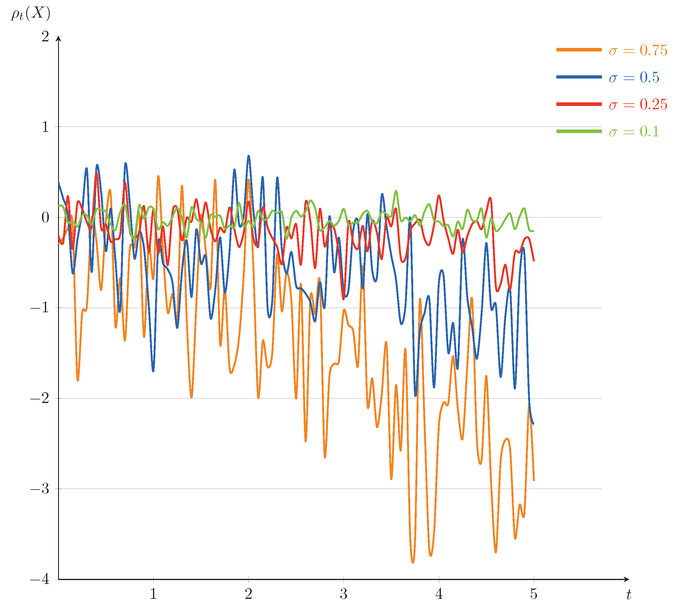
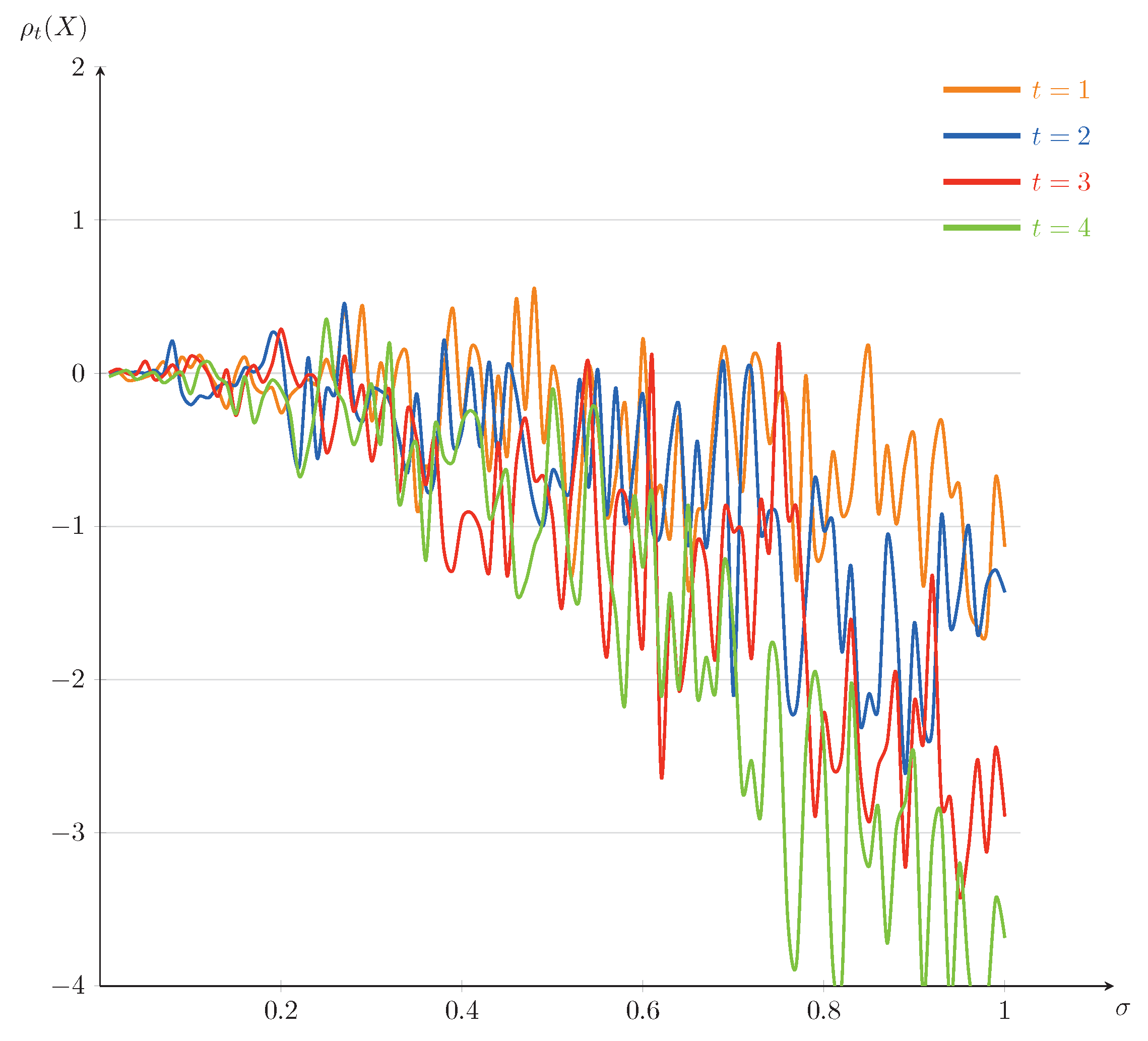
In the following, we will present some numerical illustrations for this example. Set $T=5$. The curves of ${\rho }_t\left(X\right)$ as a function of t (for $\sigma =0.1,0.25,0.5,0.75$) and as a function of $\sigma$ (for $t=1,2,3,4$) are plotted in Figure 1 and Figure 2, respectively. From Figure 1 and Figure 2, it is interesting to note that the dynamic risk measures $\rho$ tend to decline on the whole, which is consistent with our intuitive understanding: in securities trading, when the stock price drops, the loss of investors increases and the corresponding cost risk also increases, as a result, the absolute value of the dynamic risk measure becomes larger. Furthermore, we find that the values of the dynamic risk measures $\rho$ appear positive on some time interval, which can be interpreted by the effect of the large disturbance of Brownian motion at some point. We mention that the fluctuations of the dynamic risk measures $\rho$ become more stable in Figure 1 when $\sigma$ becomes smaller, and the downward trends of the dynamic risk measures $\rho$ become more obvious in Figure 2 when t becomes bigger. That is because of choosing to invest in low-risk assets and increasing of investment risk, respectively.

In a financial market, some investors may venture among certain European-type contingent claims, some bonds, some stocks, and so on. Depending on an investor’s appetite for risk, he/she may choose a curve in Figure 1 as their investment target, or choose a reasonable time of trading based on the impact of level of risk appetite in Figure 2. For example, in order to get more returns, a risk-lover may choose a curve of $\sigma =0.75$ in Figure 1 as his/her investment target in high-risk assets such as certain European-type contingent claims and some stocks. On the contrary, a risk-averse investor may choose a curve of $\sigma =0.1$ in Figure 1 as his/her investment target.

Example 2.

We suppose that the generator of the BSDEL (6) is independent of $(y,k)$ and is given by $g\left(z\right)=z^2.$ Let $X_t={\sigma }^{2}t-\sigma B_t,t\in [0,T]$, $\sigma \in (0,1]$. For any $X\in {\mathcal{S}}_T^2$ and $\sigma \in (0,1]$, we consider the following equation:

$$\begin{array}{c}\hfill Y_t=-\frac{1}{2}{X}_T+{\int }_t^{T}g\left(Z_s\right)ds-{\int }_t^T{Z}_{s}d{B}_s,t\in [0,T].\end{array}$$

(45)

The solution of (45) is

$$(Y_t,Z_t)=\left(-\frac{{\sigma }^2}{4}(T+t)+\frac{\sigma }{2}{B}_t,\frac{\sigma }{2}\right),t\in [0,T].$$

Let

$${\rho }_t\left(X\right)=-\frac{{\sigma }^2}{4}(T+t)+\frac{\sigma }{2}{B}_t,\forall t\in [0,T],X\in {\mathcal{R}}^{\infty }.$$

From Theorem 2, we obtain that $\rho$ is a dynamic convex risk measure.

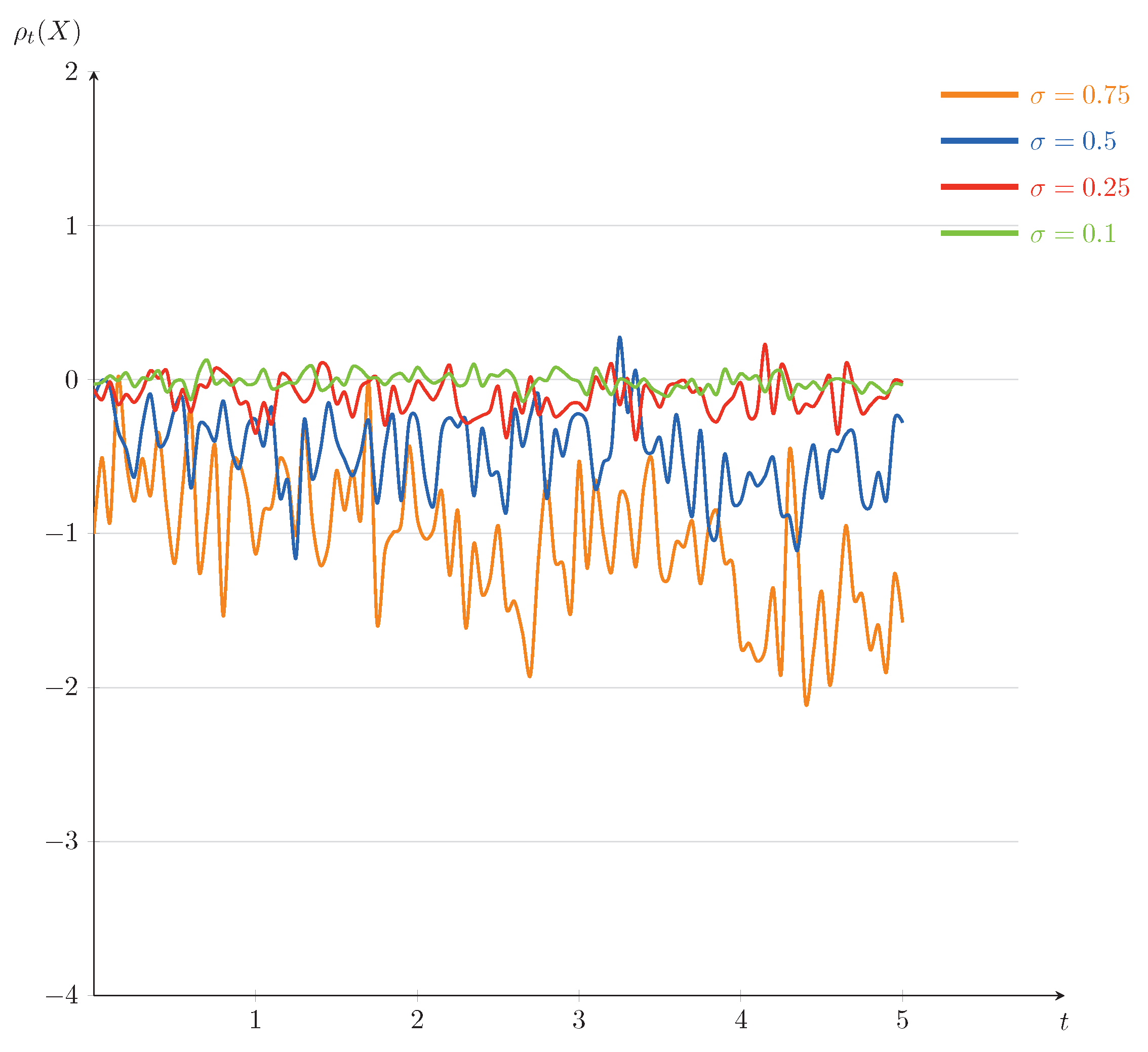
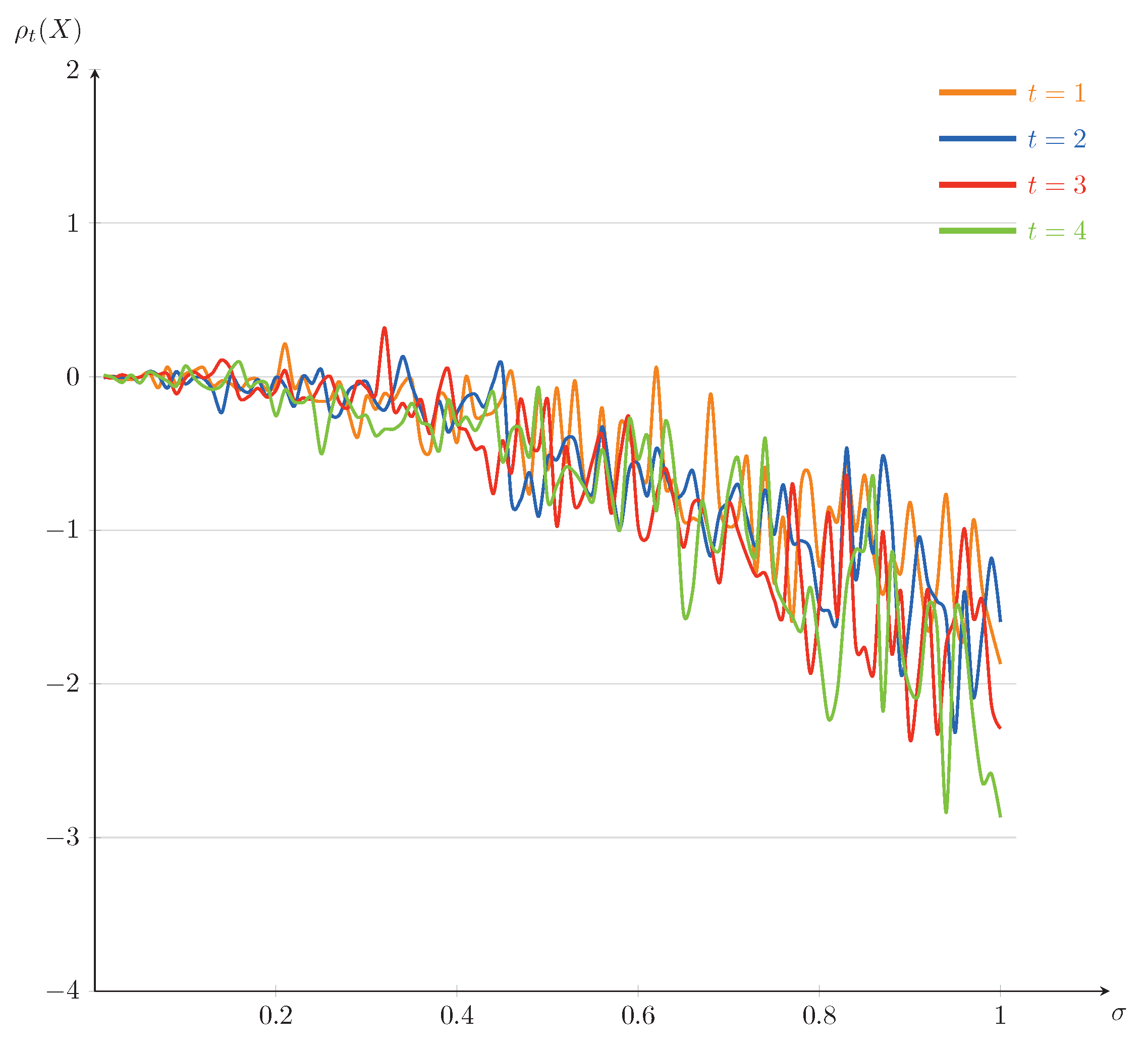
In the following, we will also present some numerical illustrations for the example. Set $T=5$. The curves of ${\rho }_t\left(X\right)$ as a function of t (for $\sigma =0.1,0.25,0.5,0.75$) and as a function of $\sigma$ (for $t=1,2,3,4$) are plotted in Figure 3 and Figure 4, respectively. It is interesting to note that, comparing with Figure 3, the downward trends of the dynamic risk measures $\rho$ are clearly obvious in Figure 4. We mention that the fluctuations of the dynamic risk measures $\rho$ become more stable in Figure 3 when $\sigma$ becomes smaller, and there are no significant differences among the dynamic risk measures $\rho$ in Figure 4 when t changes. Further, comparing Figure 3 and Figure 4 with Figure 1 and Figure 2, although the changing trends of the corresponding figures are similar, the fluctuation range of the former is smaller. This is because the solution of the current example is less affected by the diffusion term, which leads to a slower evolution speed than that of Example 1.

In a financial market, depending on investors’ appetite for risk, they may choose different investments in Figure 3. Figure 4 suggests that there may not be much difference for investors who choose a reasonable time of trading. Thus, the risk lovers, taking more risks, may choose the time $t=4$ of trading to get more returns.

6. Conclusions

In this paper, we study the dynamic risk measures for processes induced by backward stochastic differential equations driven by Teugel’s martingales associated with Lévy processes. The representation theorem for generators of BSDELs is provided. Furthermore, the time-consistency of the coherent and convex dynamic risk measures for processes is characterized by means of the generators of BSDELs. Moreover, the coherency and convexity of dynamic risk measures for processes are characterized by the generators of BSDELs. Finally, we provide two numerical examples to illustrate the proposed dynamic risk measures.

References

1. Bahlali, K.; Eddahbi, M.; Essaky, E. BSDE associated with lévy processes and application to PDIE. J. Appl. Math. Stoch. Anal. 2003, 16, 1–17. [Google Scholar] [CrossRef] [Green Version]
2. Pardoux, E.; Peng, S. Adapted solution of a backward stochastic differential equation. Syst. Control. Lett. 1990, 14, 55–61. [Google Scholar] [CrossRef]
3. Nualart, D.; Schoutens, W. Chaotic and predictable representations for Lévy processes. Stochastic Process. Appl. 2000, 90, 109–122. [Google Scholar] [CrossRef] [Green Version]
4. Nualart, D.; Schoutens, W. Backward stochastic differential equations and Feynman-Kac formula for Lévy processes, with applications in finance. Bernoulli 2001, 7, 761–776. [Google Scholar] [CrossRef] [Green Version]
5. El Otmani Mohamed. Backward stochastic differential equations associated with Lévy processes and partial integro-differential equations. Commun. Stoch. Anal. 2008, 22, 277–288. [Google Scholar]
6. El Otmani Mohamed. Reflected BSDE driven by a Lévy process. J. Theoret. Probab. 2009, 22, 601–619. [Google Scholar] [CrossRef]
7. Ren, Y.; Lin, A.; Hu, L. Stochastic PDIEs and backward doubly stochastic differential equations driven by Lévy processes. J. Comput. Appl. Math. 2009, 223, 901–907. [Google Scholar] [CrossRef] [Green Version]
8. Ren, Y.; El Otmani, M. Generalized reflected BSDEs driven by a Lévy process and an obstacle problem for PDIEs with a nonlinear Neumann boundary condition. J. Comput. Appl. Math. 2010, 233, 2027–2043. [Google Scholar] [CrossRef]
9. Briand, P.; Coquet, F.; Hu, Y.; Mémin, J.; Peng, S. A converse comparison theorem for BSDEs and related properties of g-expectation. Electron. Comm. Probab. 2000, 5, 101–117. [Google Scholar] [CrossRef]
10. Jiang, L. Representations theorems for generators of backward stochastic differential equations and their applications. Stoch. Process. Appl. 2005, 115, 1883–1903. [Google Scholar] [CrossRef] [Green Version]
11. Zhang, H.; Fan, S. A representation theorem for generators of BSDEs with finite or infinite time intervals and linear-growth generators. Statist. Probab. Lett. 2013, 83, 724–734. [Google Scholar] [CrossRef]
12. Song, L.; Hu, F.; Chen, Z. Representation theorems for generators of BSDEs in Lp spaces. Acta Math. Appl. Sin. Engl. Ser. 2012, 28, 255–264. [Google Scholar] [CrossRef]
13. Xiao, L.; Fan, S. A representation theorem for generators of BSDEs with general growth generators in y and its applications. Statist. Probab. Lett. 2018, 129, 297–305. [Google Scholar] [CrossRef] [Green Version]
14. Zheng, S.; Li, S. Representation theorem for generators of quadratic BSDEs. Acta Math. Appl. Sin. Engl. Ser. 2018, 34, 622–635. [Google Scholar] [CrossRef] [Green Version]
15. Wu, P.; Zhang, G. Representation theorems for generators of BSDEs and the extended g-expectations in probability spaces with general filtration. J. Math. Anal. Appl. 2020, 487, 124010. [Google Scholar] [CrossRef] [Green Version]
16. Artzner, P.; Delbaen, F.; Eber, J.M.; Heath, D. Thinking coherently. Risk, J. Risk Financ. 1997, 68, 68–71. [Google Scholar]
17. Artzner, P.; Delbaen, F.; Eber, J.M.; Heath, D. Coherent measures of risk. Math. Financ. 1999, 9, 203–228. [Google Scholar] [CrossRef]
18. Föllmer, H.; Schied, A. Convex measures of risk and trading constraints. Financ. Stoch. 2002, 6, 429–447. [Google Scholar] [CrossRef]
19. Frittelli, M.; Rosazza Gianin, E. Putting order in risk measures. J. Bank. Financ. 2002, 26, 1473–1486. [Google Scholar] [CrossRef]
20. Delbaen, F. Cohernet measures of risk on general probability spaces. In Advances in Finance and Stochastics; Springer: New York, NY, USA, 2002. [Google Scholar]
21. Cheridito, P.; Delbaen, F.; Kupper, M. Coherent and convex monetary risk measures for unbounded càdlàg processes. Financ. Stoch. 2005, 9, 369–387. [Google Scholar] [CrossRef]
22. Cheridito, P.; Delbaen, F.; Kupper, M. Dynamic monetary risk measures for bounded discrete time processes. Electr. J. Probab. 2006, 11, 57–106. [Google Scholar] [CrossRef]
23. Riedel, F. Dynamic coherent risk measures. Stochastic Process. Appl. 2004, 112, 185–200. [Google Scholar] [CrossRef] [Green Version]
24. Rosazza Gianin, E. Risk measures via g-expectations. Insur. Math. Econ. 2006, 39, 19–34. [Google Scholar] [CrossRef]
25. Detlefsen, K.; Scandolo, G. Conditional and dynamic convex risk measures. Financ. Stoch. 2005, 9, 539–561. [Google Scholar] [CrossRef] [Green Version]
26. Klöppel, S.; Schweizer, M. Dynamic indifference valuation via convex risk measures. Math. Financ. 2007, 17, 599–627. [Google Scholar] [CrossRef]
27. Delbaen, F.; Peng, S.; Rosazza Gianin, E. Representation of the penalty term of dynamic concave utilities. Financ. Stoch. 2010, 14, 449–472. [Google Scholar] [CrossRef]
28. Acciaio, B.; Föllmer, H.; Penner, I. Risk assessment for uncertain cash flows: Model ambiguity, discounting ambiguity, and the role of bubbles. Financ. Stoch. 2012, 16, 669–709. [Google Scholar] [CrossRef] [Green Version]
29. Föllmer, H.; Schied, A. Stochastic Finance: An Introduction in Discrete Time, 4nd revised and extended ed.; Welter de Gruyter: Berlin, Germany; New York, NY, USA, 2016. [Google Scholar]
30. Song, H.; Zeng, X.; Chen, Y.; Hu, Y. Multivariate shortfall and divergence risk statistics. Entropy 2019, 21, 1031. [Google Scholar] [CrossRef] [Green Version]
31. Peng, S. Backward SDE and related g-expectation. Pitman Res. Notes Math. Ser. 1997, 364, 141–159. [Google Scholar]
32. El Karoui, N.; Peng, S.; Quenez, M.C. Backward stochastic differential equations in finance. Math. Financ. 1997, 7, 1–71. [Google Scholar] [CrossRef]
33. Jiang, L. Convexity, translation invariance and subadditivity for g-expectations and related risk measures. Ann. Appl. Probab. 2008, 18, 245–258. [Google Scholar] [CrossRef]
34. Penner, I.; Réveillac, A. Risk measure for processes and BSDEs. Financ. Stoch. 2015, 19, 23–66. [Google Scholar] [CrossRef] [Green Version]
35. Xu, Y. Multidimensional dynamic risk measures via conditional g-expectation. Math. Financ. 2016, 26, 638–673. [Google Scholar] [CrossRef] [Green Version]
36. Ji, R.; Shi, X.; Wang, S.; Zhou, J. Dynamic risk measures for processes via backward stochastic differentical equations. Insur. Math. Econ. 2019, 86, 43–50. [Google Scholar] [CrossRef]
37. Bion-Nadal, J. Dynamic risk measures: Time consistency and risk measures from BMO martingale. Financ. Stoch. 2008, 12, 219–244. [Google Scholar] [CrossRef]
38. Bion-Nadal, J. Time consistent dynamic risk processes. Stoch. Proc. Appl. 2009, 119, 633–654. [Google Scholar] [CrossRef] [Green Version]
39. Yong, J. Continuous-time dynamic risk measures by backward stochastic Volterra integral equations. Appl. Anal. 2007, 86, 1429–1442. [Google Scholar] [CrossRef]
40. Wang, T.; Shi, Y. A class of time inconsistent risk measures and backward stochastic Volterra integral equations. Risk Decis. Anal. 2013, 4, 17–24. [Google Scholar] [CrossRef]
41. Agram, N. Dynamic risk measure for BSVIE with jumps and semimartinggale issues. Stoch. Anal. appl. 2019, 37, 361–376. [Google Scholar] [CrossRef] [Green Version]
42. Barles, G.; Buckdahn, R.; Pardoux, E. Backward stochastic differential equations and integral-partial differential equations. Stochastics Stochastics Rep. 1997, 60, 57–83. [Google Scholar] [CrossRef]
43. Protter, P. Stochastic Integration and Differential Equations; Springer: Berlin, Germany, 1990. [Google Scholar]
44. Zhang, J. Backward Stochastic Differential Equations: From Linear to Fully Nonlinear Theory; Springer: New York, NY, USA, 2017. [Google Scholar]
Figure 1. The trends of ρ t ( X ) as a funtion of t for Example 1 (fixed σ = 0.1 , 0.25 , 0.5 , 0.75 ).
Entropy 23 00741 g001
Figure 2. The trends of ρ t ( X ) as a funtion of σ for Example 1 (fixed t = 1 , 2 , 3 , 4 ).
Entropy 23 00741 g002
Figure 3. The trends of ρ t ( X ) as a function of t for Example 2 (fixed σ = 0.1 , 0.25 , 0.5 , 0.75 ).
Entropy 23 00741 g003
Figure 4. The trends of ρ t ( X ) as a function of σ for Example 2(fixed t = 1 , 2 , 3 , 4 ).
Entropy 23 00741 g004
Publisher’s Note: MDPI stays neutral with regard to jurisdictional claims in published maps and institutional affiliations.