
Entropy and Multifractal-Multiscale Indices of Heart Rate Time Series to Evaluate Intricate Cognitive-Autonomic Interactions


Abstract
:1. Introduction
2. Materials and Methods
2.1. Population
2.2. Experimental Design
2.3. Cognitive Tasks
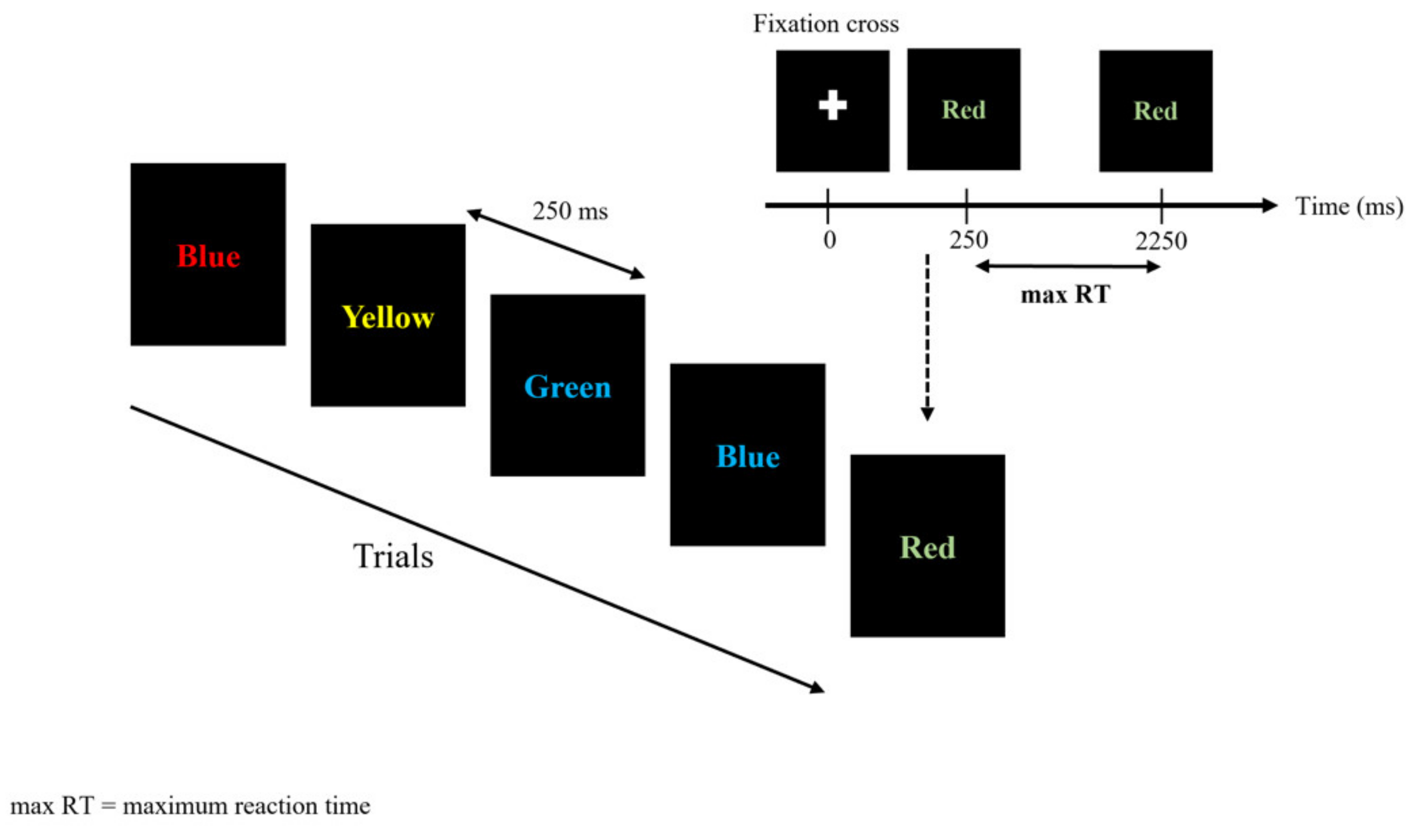
2.3.1. Stroop Color and Word Task (SCWT)
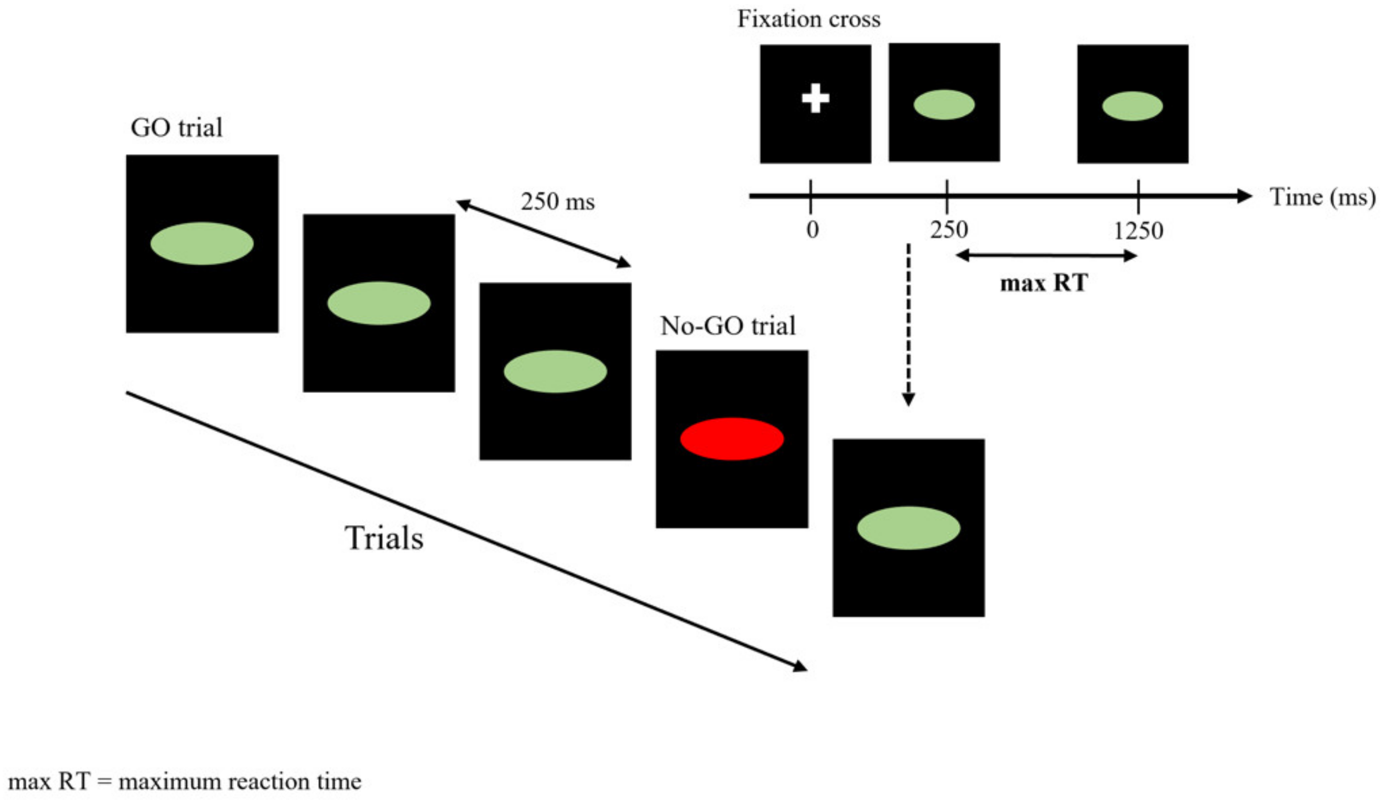
2.3.2. Go/No-Go Task (GNGT)
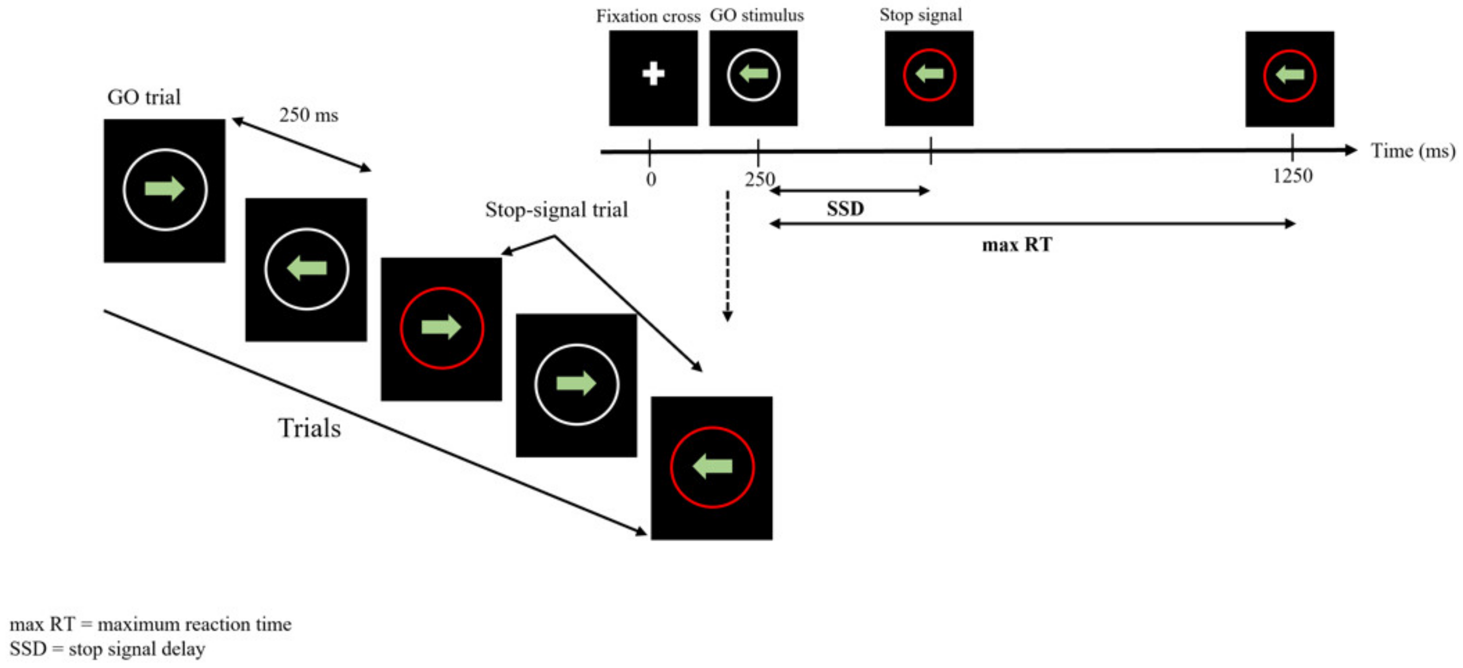
2.3.3. Stop Signal Task (SST)
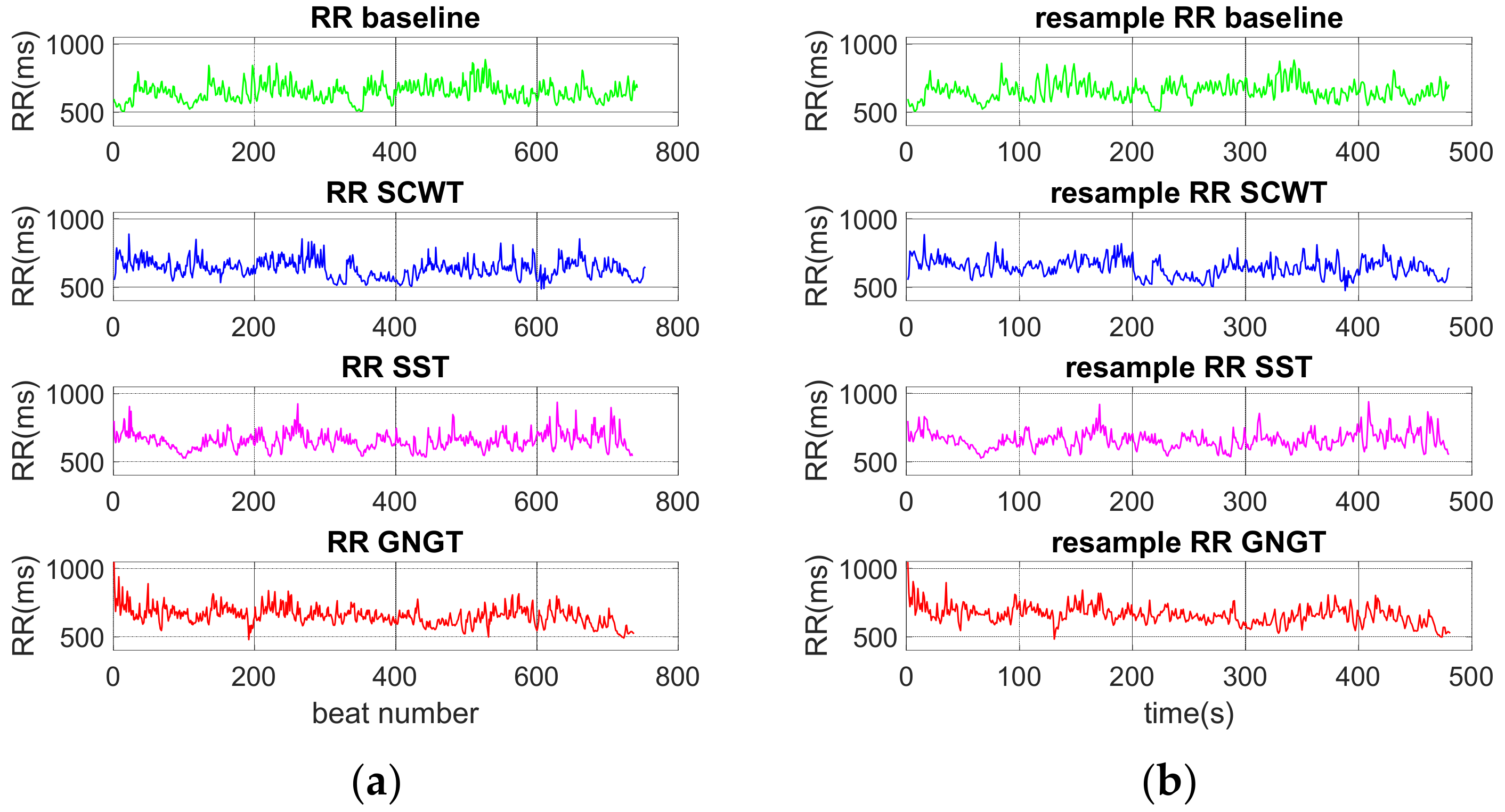
2.4. Analysis of RR Time Series
2.4.1. Time and Frequency Domains Analyses
2.4.2. Entropy in RR Time Series
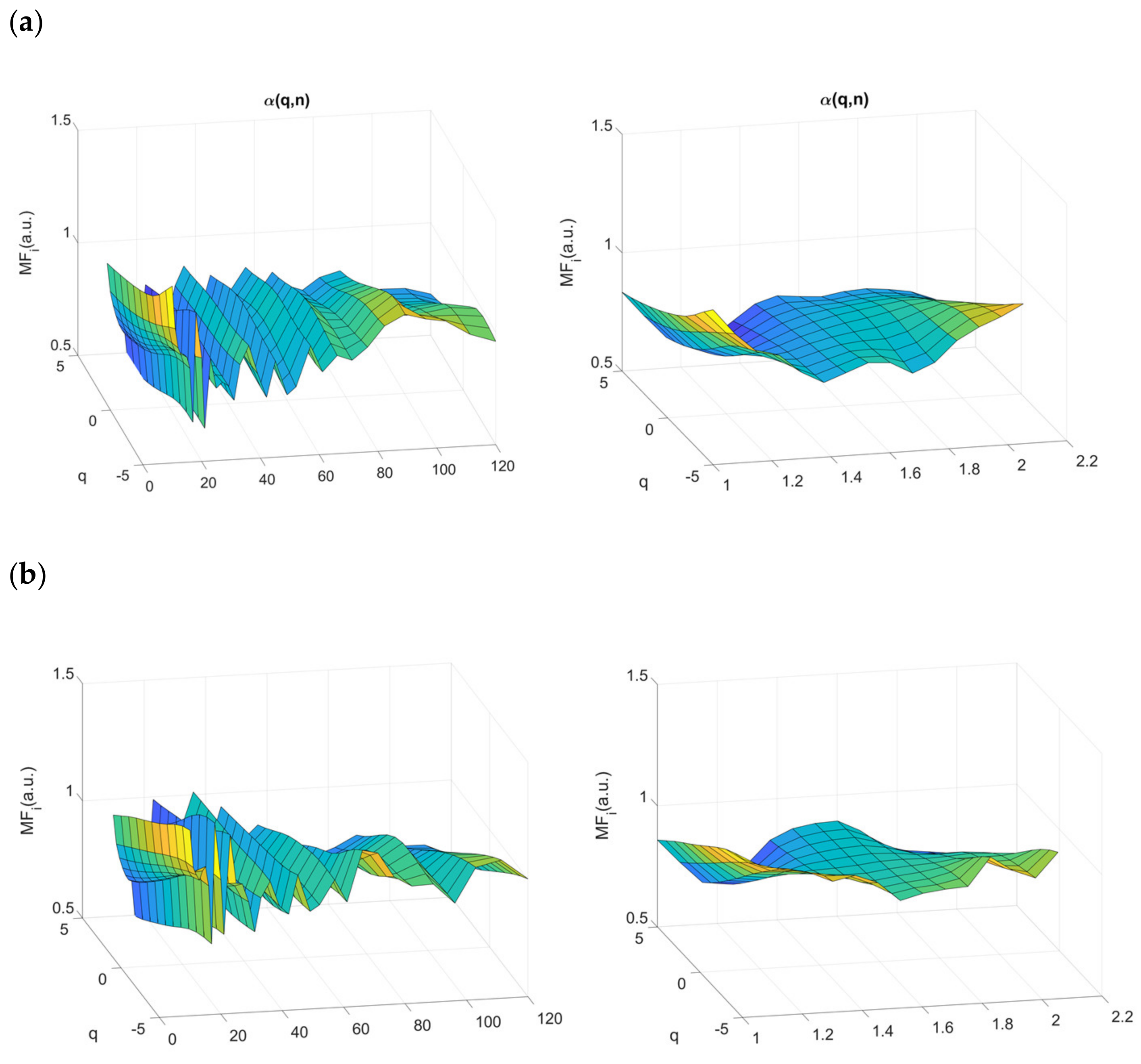
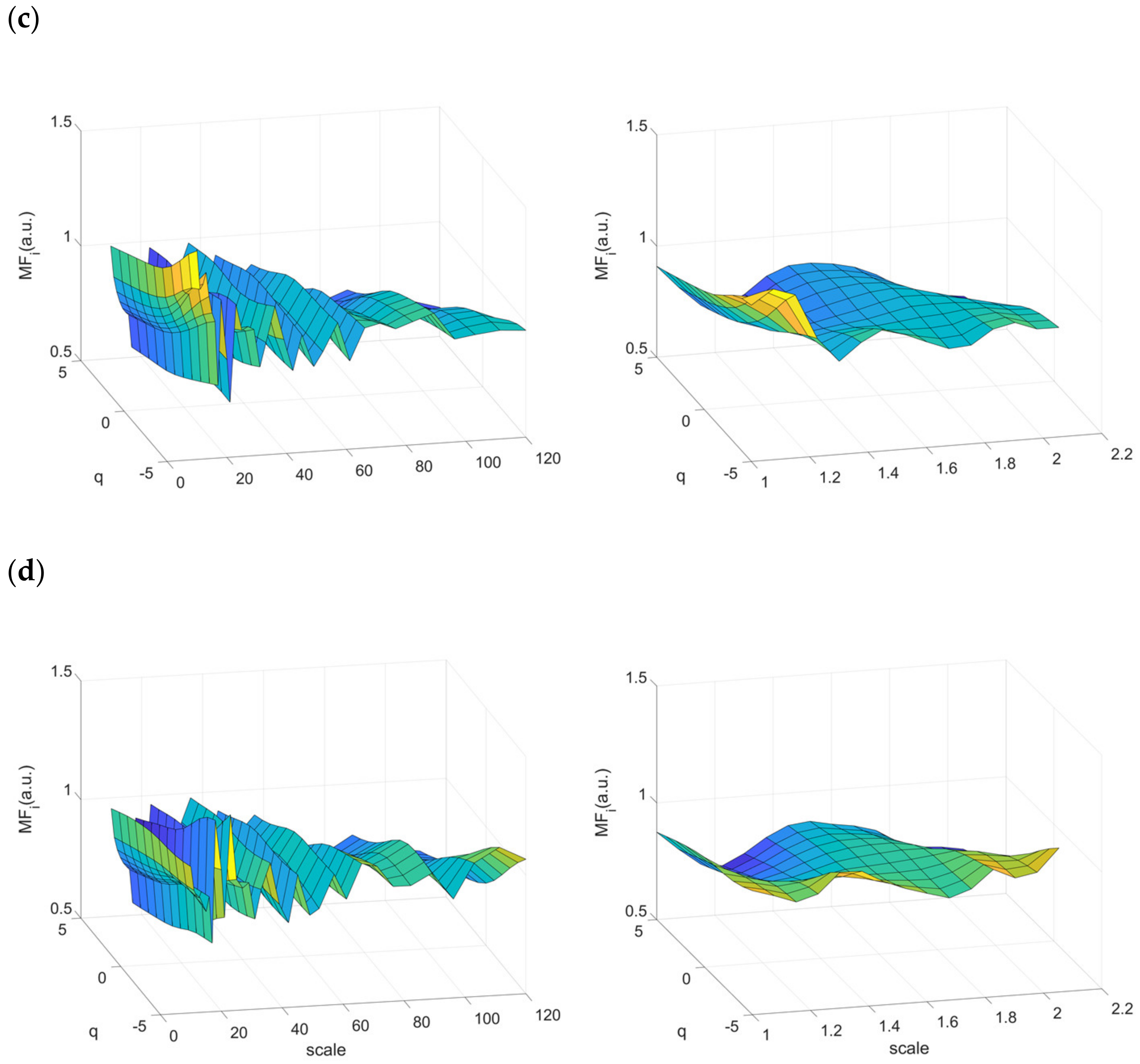
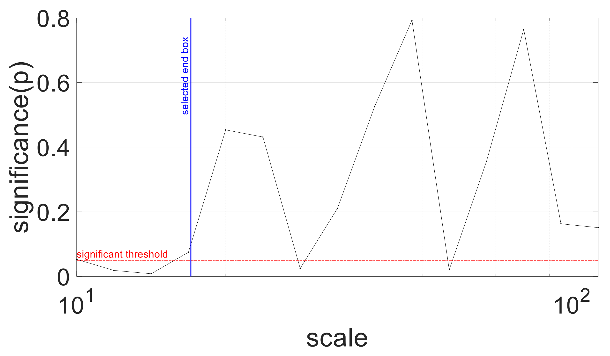
2.4.3. Multifractal Properties of RR Time Series
2.5. Statistical Analysis
3. Results
3.1. Cognitive Performance: Response Time and Accuracy
3.2. Classical Metrics in RR Time Series
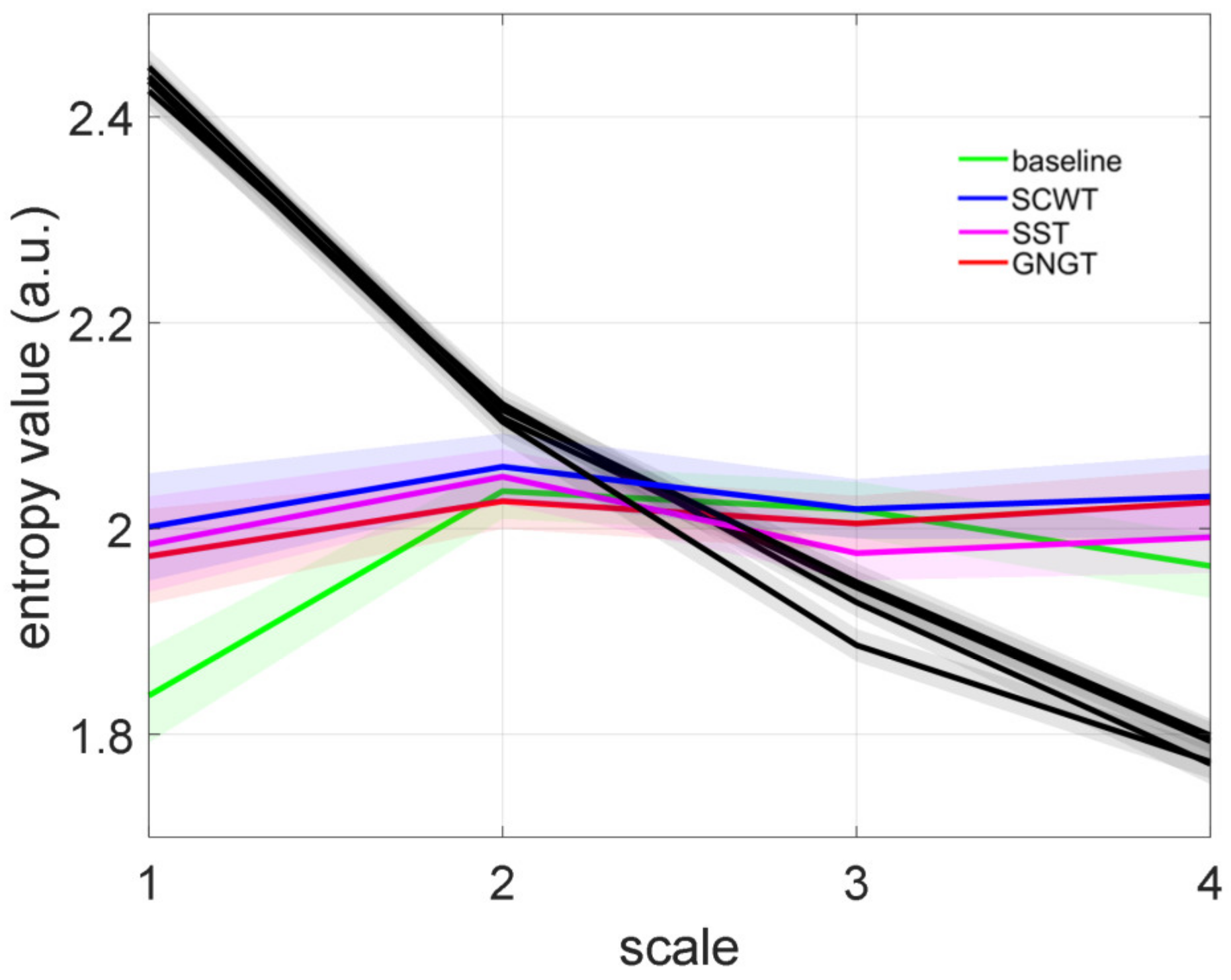
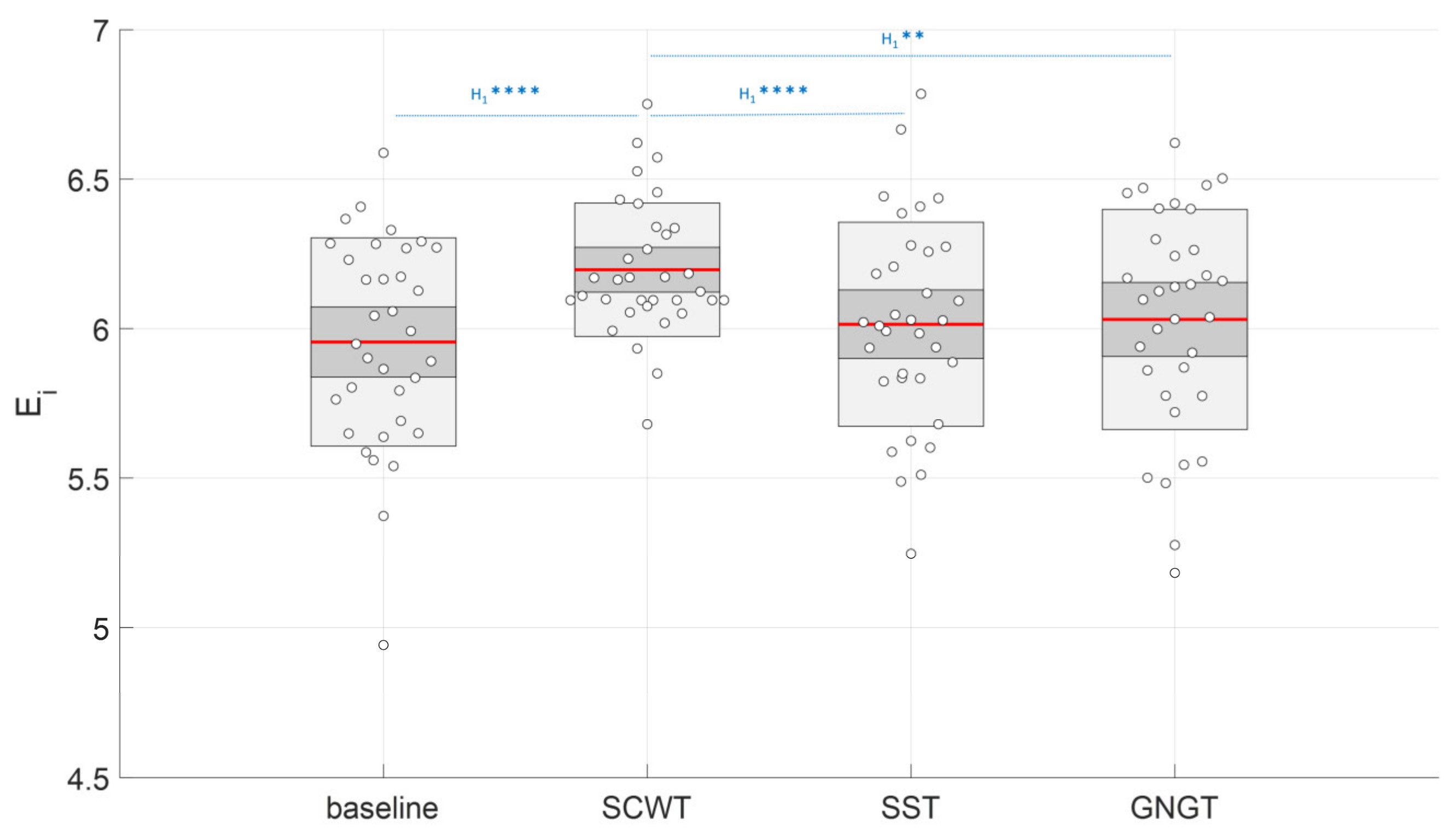
3.3. Multiscale Entropy in RR Time Series
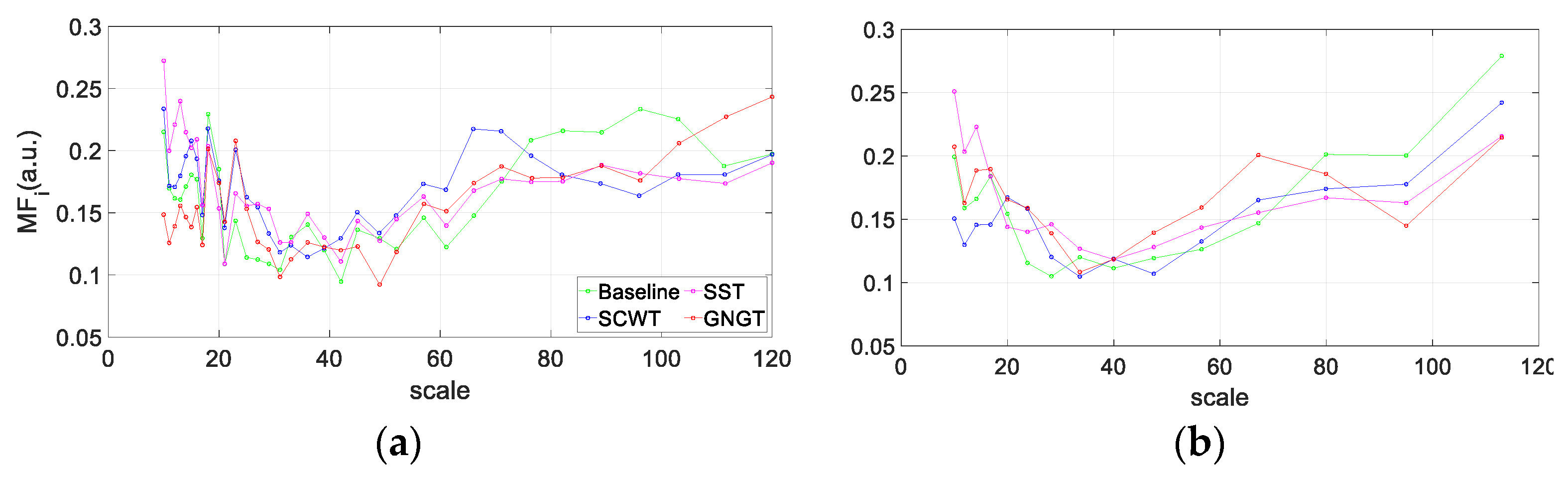
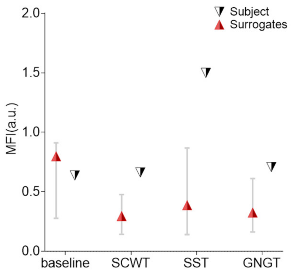
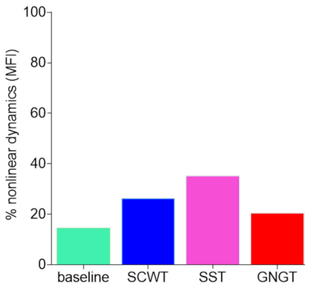
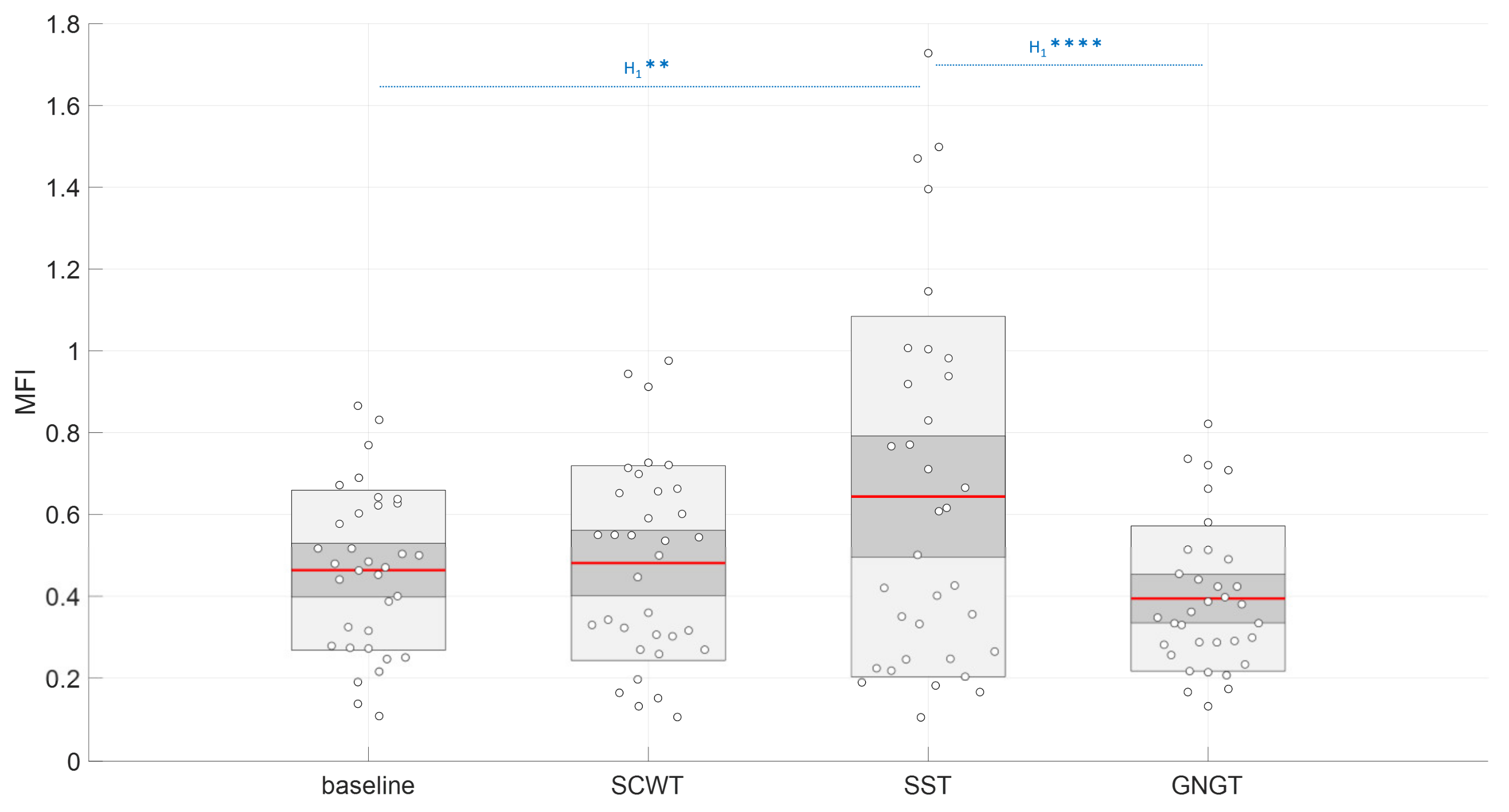
3.4. Multifractality in RR Time Series
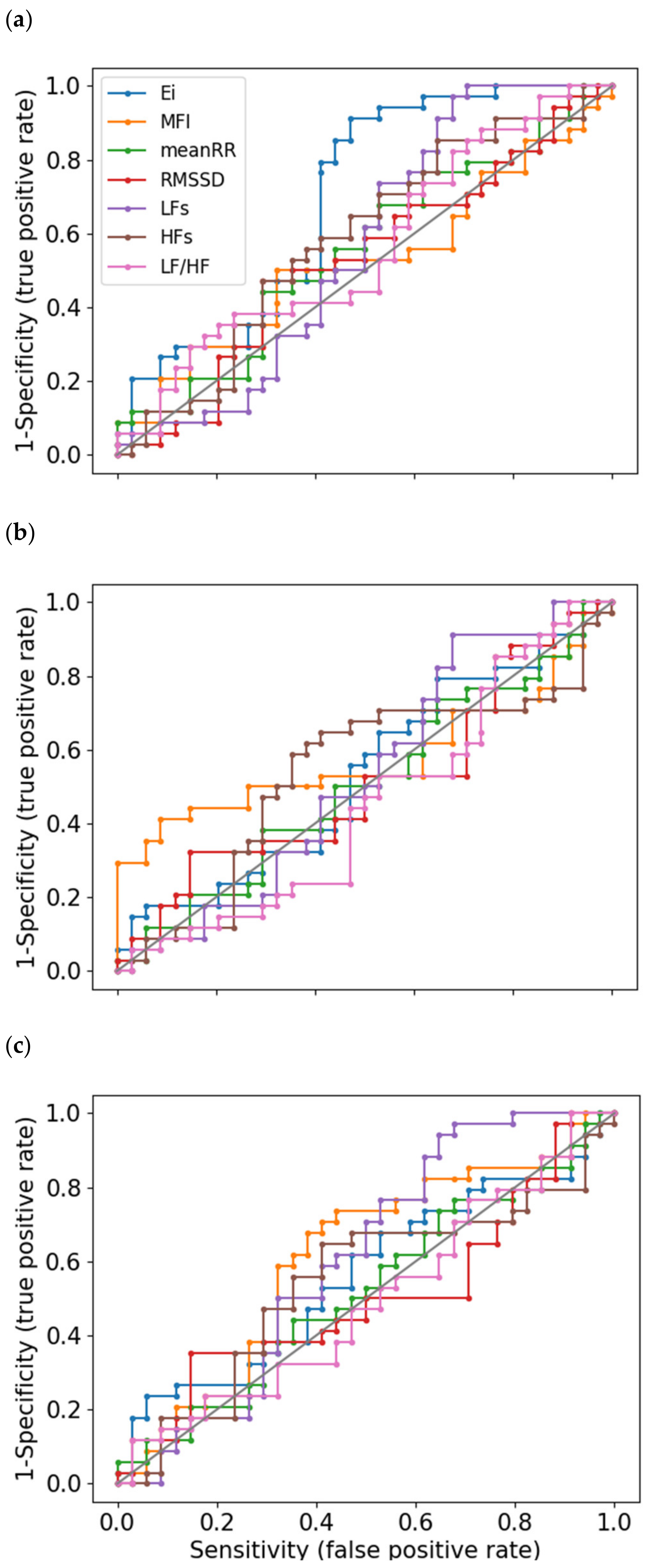
3.5. Sensitivity Analysis: ROC Curves
4. Discussion
4.1. A Cognitive Architecture Reflected in HRV Time Series
4.2. Specificity of the Nonlinear Metrics
4.3. Improved Entropy in SCWT
4.4. Multifractality in SST
5. Conclusions
Supplementary Materials
Author Contributions
Funding
Institutional Review Board Statement
Informed Consent Statement
Data Availability Statement
Conflicts of Interest
References
- Costa, M.; Goldberger, A.L.; Peng, C.-K. Multiscale Entropy Analysis of Complex Physiologic Time Series. Phys. Rev. Lett. 2002, 89, 068102. [Google Scholar] [CrossRef] [PubMed] [Green Version]
- Lipsitz, L.A. Dynamics of Stability: The Physiologic Basis of Functional Health and Frailty. J. Gerontol. Ser. A Biol. Sci. Med Sci. 2002, 57, B115–B125. [Google Scholar] [CrossRef] [PubMed] [Green Version]
- Costa, M.; Goldberger, A.L.; Peng, C.-K. Multiscale Entropy Analysis of Biological Signals. Phys. Rev. E Stat. Nonlin. Soft Matter Phys. 2005, 71, 021906. [Google Scholar] [CrossRef] [PubMed] [Green Version]
- Wayne, P.M.; Gow, B.J.; Costa, M.D.; Peng, C.-K.; Lipsitz, L.A.; Hausdorff, J.M.; Davis, R.B.; Walsh, J.N.; Lough, M.; Novak, V.; et al. Complexity-Based Measures Inform Effects of Tai Chi Training on Standing Postural Control: Cross-Sectional and Randomized Trial Studies. PLoS ONE 2014, 9, e114731. [Google Scholar] [CrossRef] [Green Version]
- Benarroch, E.E. The Central Autonomic Network: Functional Organization, Dysfunction, and Perspective. Mayo Clin. Proc. 1993, 68, 988–1001. [Google Scholar] [CrossRef]
- Thayer, J.F.; Lane, R.D. A Model of Neurovisceral Integration in Emotion Regulation and Dysregulation. J. Affect. Disord. 2000, 61, 201–216. [Google Scholar] [CrossRef] [Green Version]
- Valenza, G.; Sclocco, R.; Duggento, A.; Passamonti, L.; Napadow, V.; Barbieri, R.; Toschi, N. The Central Autonomic Network at Rest: Uncovering Functional MRI Correlates of Time-Varying Autonomic Outflow. NeuroImage 2019, 197, 383–390. [Google Scholar] [CrossRef]
- Mather, M.; Thayer, J. How Heart Rate Variability Affects Emotion Regulation Brain Networks. Curr. Opin. Behav. Sci. 2018, 19, 98–104. [Google Scholar] [CrossRef]
- Young, H.; Benton, D. We Should Be Using Nonlinear Indices When Relating Heart-Rate Dynamics to Cognition and Mood. Sci. Rep. 2015, 5, 16619. [Google Scholar] [CrossRef] [Green Version]
- Dimitriev, D.A.; Saperova, E.V.; Dimitriev, A.D. State Anxiety and Nonlinear Dynamics of Heart Rate Variability in Students. PLoS ONE 2016, 11, e0146131. [Google Scholar] [CrossRef] [Green Version]
- Wu, S.-D.; Wu, C.-W.; Lin, S.-G.; Lee, K.-Y.; Peng, C.-K. Analysis of Complex Time Series Using Refined Composite Multiscale Entropy. Phys. Lett. A 2014, 378, 1369–1374. [Google Scholar] [CrossRef]
- Faes, L.; Porta, A.; Javorka, M.; Nollo, G. Efficient Computation of Multiscale Entropy over Short Biomedical Time Series Based on Linear State-Space Models. Complexity 2017, 2017, e1768264. [Google Scholar] [CrossRef]
- Blons, E.; Arsac, L.; Gilfriche, P.; Deschodt-Arsac, V. Multiscale Entropy of Cardiac and Postural Control Reflects a Flexible Adaptation to a Cognitive Task. Entropy 2019, 21, 1024. [Google Scholar] [CrossRef] [Green Version]
- Blons, E.; Arsac, L.M.; Gilfriche, P.; McLeod, H.; Lespinet-Najib, V.; Grivel, E.; Deschodt-Arsac, V. Alterations in Heart-Brain Interactions under Mild Stress during a Cognitive Task Are Reflected in Entropy of Heart Rate Dynamics. Sci. Rep. 2019, 9, 18190. [Google Scholar] [CrossRef] [PubMed]
- Deschodt-Arsac, V.; Blons, E.; Gilfriche, P.; Spiluttini, B.; Arsac, L.M. Entropy in Heart Rate Dynamics Reflects How HRV-Biofeedback Training Improves Neurovisceral Complexity during Stress-Cognition Interactions. Entropy 2020, 22, 317. [Google Scholar] [CrossRef] [PubMed] [Green Version]
- Castiglioni, P.; Lazzeroni, D.; Coruzzi, P.; Faini, A. Multifractal-Multiscale Analysis of Cardiovascular Signals: A DFA-Based Characterization of Blood Pressure and Heart-Rate Complexity by Gender. Complexity 2018, 2018, 1–14. [Google Scholar] [CrossRef] [Green Version]
- Castiglioni, P.; Parati, G.; Civijian, A.; Quintin, L.; Rienzo, M.D. Local Scale Exponents of Blood Pressure and Heart Rate Variability by Detrended Fluctuation Analysis: Effects of Posture, Exercise, and Aging. IEEE Trans. Biomed. Eng. 2009, 56, 10. [Google Scholar] [CrossRef]
- Torre, K.; Vergotte, G.; Viel, É.; Perrey, S.; Dupeyron, A. Fractal Properties in Sensorimotor Variability Unveil Internal Adaptations of the Organism before Symptomatic Functional Decline. Sci. Rep. 2019, 9, 15736. [Google Scholar] [CrossRef]
- Stoet, G. PsyToolkit: A Novel Web-Based Method for Running Online Questionnaires and Reaction-Time Experiments. Teach. Psychol. 2017, 44, 24–31. [Google Scholar] [CrossRef]
- Stoet, G. PsyToolkit: A Software Package for Programming Psychological Experiments Using Linux. Behav. Res. Methods 2010, 42, 1096–1104. [Google Scholar] [CrossRef]
- Stroop, J.R. Studies of Interference in Serial Verbal Reactions. J. Exp. Psychol. 1935, 18, 643–662. [Google Scholar] [CrossRef]
- Littman, R.; Takács, Á. Do All Inhibitions Act Alike? A Study of Go/No-Go and Stop-Signal Paradigms. PLoS ONE 2017, 12, e0186774. [Google Scholar] [CrossRef] [PubMed] [Green Version]
- Raud, L.; Westerhausen, R.; Dooley, N.; Huster, R.J. Differences in Unity: The Go/No-Go and Stop Signal Tasks Rely on Different Mechanisms. NeuroImage 2020, 210, 116582. [Google Scholar] [CrossRef]
- Logan, G.D.; Cowan, W.B. On the Ability to Inhibit Thought and Action: A Theory of an Act of Control. Psychol. Rev. 1984, 121, 66–95. [Google Scholar] [CrossRef] [PubMed] [Green Version]
- Logan, G.D.; Schachar, R.J.; Tannock, R. Impulsivity and Inhibitory Control. Psychol. Sci. 1997, 8, 60–64. [Google Scholar] [CrossRef] [Green Version]
- Verbruggen, F.; Logan, G.D. Models of Response Inhibition in the Stop-Signal and Stop-Change Paradigms. Neurosci. Biobehav. Rev. 2009, 33, 647–661. [Google Scholar] [CrossRef] [PubMed] [Green Version]
- Pasadyn, S.R.; Soudan, M.; Gillinov, M.; Houghtaling, P.; Phelan, D.; Gillinov, N.; Bittel, B.; Desai, M.Y. Accuracy of Commercially Available Heart Rate Monitors in Athletes: A Prospective Study. Cardiovasc. Diagn. Ther. 2019, 9, 379–385. [Google Scholar] [CrossRef] [PubMed]
- Gilgen-Ammann, R.; Schweizer, T.; Wyss, T. RR Interval Signal Quality of a Heart Rate Monitor and an ECG Holter at Rest and during Exercise. Eur. J. Appl. Physiol. 2019, 119, 1525–1532. [Google Scholar] [CrossRef]
- Electrophysiology Task Force of the European Society of Cardiology the North American Society of Pacing Heart Rate Variability. Circulation 1996, 93, 1043–1065. [CrossRef] [Green Version]
- Gow, B.; Peng, C.-K.; Wayne, P.; Ahn, A. Multiscale Entropy Analysis of Center-of-Pressure Dynamics in Human Postural Control: Methodological Considerations. Entropy 2015, 17, 7926–7947. [Google Scholar] [CrossRef]
- Porta, A.; D’Addio, G.; Guzzetti, S.; Lucini, D.; Pagani, M. Testing the Presence of Non Stationarities in Short Heart Rate Variability Series. In Proceedings of the Computers in Cardiology, Chicago, IL, USA, 19–22 September 2004; pp. 645–648. [Google Scholar]
- Magagnin, V.; Bassani, T.; Bari, V.; Turiel, M.; Maestri, R.; Pinna, G.D.; Porta, A. Non-Stationarities Significantly Distort Short-Term Spectral, Symbolic and Entropy Heart Rate Variability Indices. Physiol. Meas. 2011, 32, 1775–1786. [Google Scholar] [CrossRef]
- Schreiber, T.; Schmitz, A. Improved Surrogate Data for Nonlinearity Tests. Phys. Rev. Lett. 1996, 77, 635–638. [Google Scholar] [CrossRef] [PubMed] [Green Version]
- Faes, L.; Gómez-Extremera, M.; Pernice, R.; Carpena, P.; Nollo, G.; Porta, A.; Bernaola-Galván, P. Comparison of Methods for the Assessment of Nonlinearity in Short-Term Heart Rate Variability under Different Physiopathological States. Chaos 2019, 29, 123114. [Google Scholar] [CrossRef] [PubMed] [Green Version]
- Porta, A.; Bari, V.; De Maria, B.; Cairo, B.; Vaini, E.; Malacarne, M.; Pagani, M.; Lucini, D. On the Relevance of Computing a Local Version of Sample Entropy in Cardiovascular Control Analysis. IEEE Trans. Biomed. Eng. 2019, 66, 623–631. [Google Scholar] [CrossRef]
- Faes, L.; Marinazzo, D.; Montalto, A.; Nollo, G. Lag-Specific Transfer Entropy as a Tool to Assess Cardiovascular and Cardiorespiratory Information Transfer. IEEE Trans. Biomed. Eng. 2014, 61, 2556–2568. [Google Scholar] [CrossRef] [PubMed]
- Xiong, W.; Faes, L.; Ivanov, P.C. Entropy Measures, Entropy Estimators, and Their Performance in Quantifying Complex Dynamics: Effects of Artifacts, Nonstationarity, and Long-Range Correlations. Phys. Rev. E 2017, 95, 062114. [Google Scholar] [CrossRef] [PubMed] [Green Version]
- Faes, L.; Kugiumtzis, D.; Nollo, G.; Jurysta, F.; Marinazzo, D. Estimating the Decomposition of Predictive Information in Multivariate Systems. Phys. Rev. E 2015, 91, 032904. [Google Scholar] [CrossRef] [PubMed] [Green Version]
- Peng, C.K.; Havlin, S.; Stanley, H.E.; Goldberger, A.L. Quantification of Scaling Exponents and Crossover Phenomena in Nonstationary Heartbeat Time Series. Chaos 1995, 5, 82–87. [Google Scholar] [CrossRef]
- Castiglioni, P. A Fast DFA Algorithm for Multifractal Multiscale Analysis of Physiological Time Series. Front. Physiol. 2019, 10, 18. [Google Scholar] [CrossRef] [PubMed] [Green Version]
- Keysers, C.; Gazzola, V.; Wagenmakers, E.-J. Using Bayes Factor Hypothesis Testing in Neuroscience to Establish Evidence of Absence. Nat. Neurosci. 2020, 23, 788–799. [Google Scholar] [CrossRef]
- Rouder, J.N.; Speckman, P.L.; Sun, D.; Morey, R.D.; Iverson, G. Bayesian t Tests for Accepting and Rejecting the Null Hypothesis. Psychon. Bull. Rev. 2009, 16, 225–237. [Google Scholar] [CrossRef] [PubMed]
- Wagenmakers, E.-J. Bayesian Inference for Psychology. Part II: Example Applications with JASP. Psychon. Bull. Rev. 2018, 25, 58–76. [Google Scholar] [CrossRef] [PubMed] [Green Version]
- Jeffreys, H. Theory of Probability, 3rd ed.; Oxford University Press: Oxford, UK, 1961. [Google Scholar]
- Metz, C.E. Basic Principles of ROC Analysis. Semin. Nucl. Med. 1978, 8, 283–298. [Google Scholar] [CrossRef]
- Hanley, J.A.; McNeil, B.J. The Meaning and Use of the Area under a Receiver Operating Characteristic (ROC) Curve. Radiology 1982, 143, 29–36. [Google Scholar] [CrossRef] [PubMed] [Green Version]
- Vergotte, G.; Perrey, S.; Muthuraman, M.; Janaqi, S.; Torre, K. Concurrent Changes of Brain Functional Connectivity and Motor Variability When Adapting to Task Constraints. Front. Physiol. 2018, 9, 909. [Google Scholar] [CrossRef]
- Luque-Casado, A.; Perakakis, P.; Ciria, L.F.; Sanabria, D. Transient Autonomic Responses during Sustained Attention in High and Low Fit Young Adults. Sci. Rep. 2016, 6, 27556. [Google Scholar] [CrossRef]
- Ihlen, E.A.F.; Vereijken, B. Interaction-Dominant Dynamics in Human Cognition: Beyond 1/f(Alpha) Fluctuation. J. Exp. Psychol. Gen. 2010, 139, 436–463. [Google Scholar] [CrossRef]
- Stephen, D.G.; Dixon, J.A.; Isenhower, R.W. Dynamics of Representational Change: Entropy, Action, and Cognition. J. Exp. Psychol. Hum. Percept Perform 2009, 35, 1811–1832. [Google Scholar] [CrossRef]
- Van Orden, G.C.; Holden, J.G.; Turvey, M.T. Self-Organization of Cognitive Performance. J. Exp. Psychol. Gen. 2003, 132, 331–350. [Google Scholar] [CrossRef] [Green Version]
- Kim, C.; Johnson, N.F.; Gold, B.T. Conflict Adaptation in Prefrontal Cortex: Now You See It, Now You Don’t. Cortex 2014, 50, 76–85. [Google Scholar] [CrossRef] [Green Version]
- Friehs, M.A.; Klaus, J.; Singh, T.; Frings, C.; Hartwigsen, G. Perturbation of the Right Prefrontal Cortex Disrupts Interference Control. Neuroimage 2020, 222, 117279. [Google Scholar] [CrossRef] [PubMed]
- Thayer, J.F.; Saus-Rose, E.; Johnsen, B.H. Heart Rate Variability, Prefrontal Neural Function, and Cognitive Performance: The Neurovisceral Integration Perspective on Self-Regulation, Adaptation, and Health. Ann. Behav. Med. 2009, 37, 141–153. [Google Scholar] [CrossRef] [PubMed]


| Variable (Unit) | SCWT | SST | GNGT |
|---|---|---|---|
| RT (ms) | 879 ± 119 c | 496 ± 69 c | 405 ± 64 * |
| perf (%) | 97.0 ± 2.25 | 99.3 ± 0.83 | 97.6 ± 1.80 |
| SSRT (ms) | 308 ± 32.4 | ||
| inhib perf (%) | 60.4 ± 22.7 |
| Variable (Unit) | Baseline | SCWT | SST | GNGT |
|---|---|---|---|---|
| meanRR (ms) | 841 ± 131c | 812 ± 131 * | 836 ± 131 c | 832 ± 135 c |
| RMSSD (ms) | 43.3 ± 18.9 | 42.0 ± 18.1 | 45.3 ± 21.1 | 44.7 ± 21.7 |
| LF (ms^2/Hz) | 1471 ± 927 | 1165 ± 462 | 1291 ± 643 | 1064 ± 463 |
| HF (ms^2/Hz) | 886 ± 630 | 685 ± 515 | 862 ± 777 | 862 ± 761 |
| LF/HF | 2.25 ± 1.69 | 2.62 ± 1.95 | 2.23 ± 1.19 | 2.23 ±1.51 |
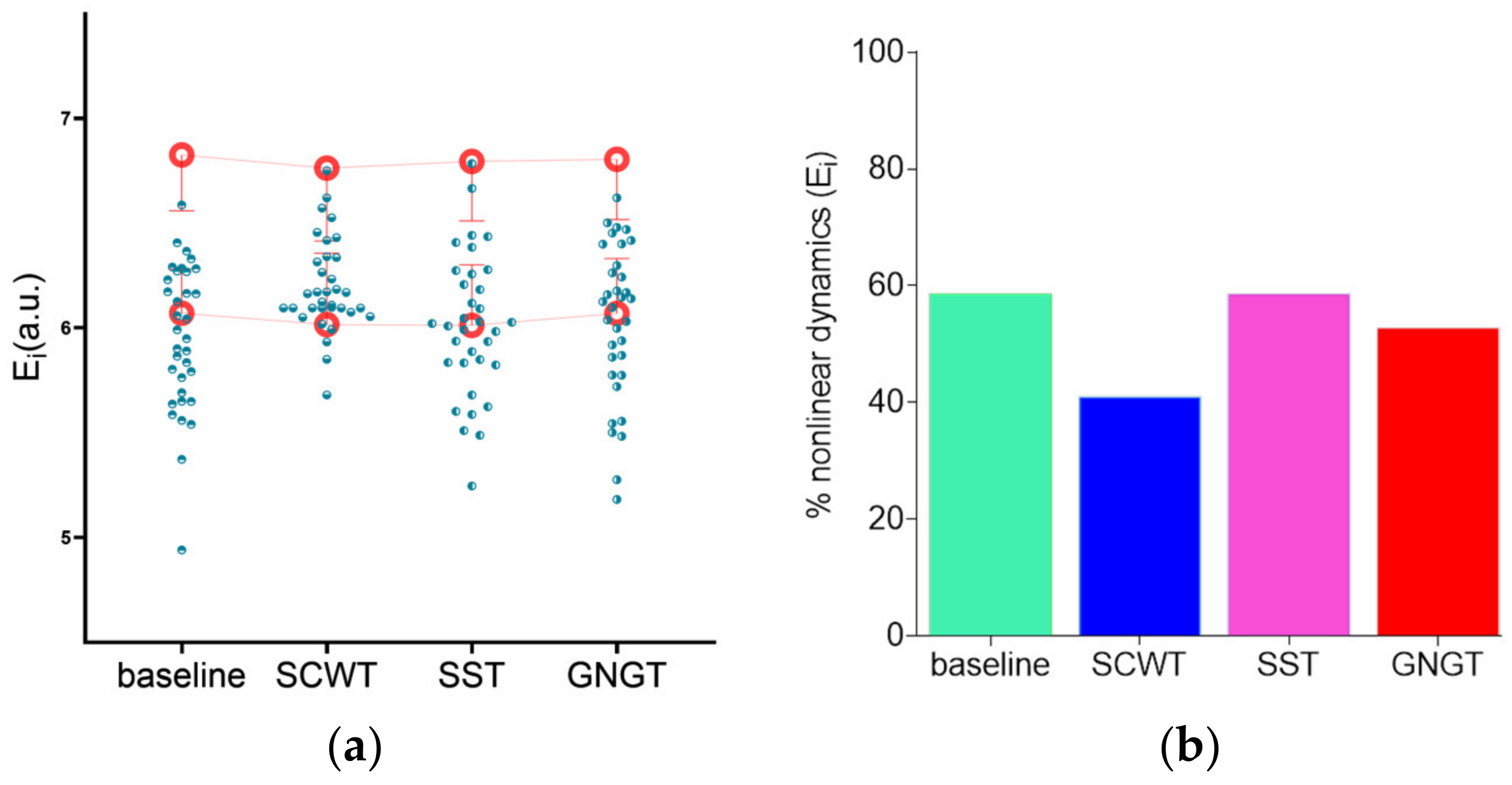
| Ei (a.u.) | 5.96 ± 0.35 c | 6.20 ± 0.22 * | 6.01 ± 0.34 c | 6.03 ± 0.37 c |
| MFI (a.u.) | 0.46 ± 0.20 c | 0.48 ± 0.24 | 0.64 ± 0.44 * | 0.39- ± 0.18 c |
| Entropy Indices (Unit) | Baseline | SCWT | SST | GNGT |
|---|---|---|---|---|
| LMSE (a.u.) | 2.90 ± 0.52 | 3.19 ± 0.44 | 3.09 ± 0.52 | 3.09 ± 0.48 |
| CEBi (a.u.) | 1.02 ± 0.11 | 1.00 ± 0.16 | 1.03 ± 0.15 | 1.01 ± 0.16 |
| CEKe (a.u.) | 1.84 ± 0.27 | 2.00 ± 0.30 | 1.98 ± 0.27 | 1.98 ± 0.20 |
| CENN (a.u.) | 5.31 ± 0.30 | 5.27 ± 0.27 | 5.34 ± 0.28 | 5.25 ± 0.35 |
| Indices | SCWT/Baseline | SST/Baseline | GNGT/Baseline | |||
|---|---|---|---|---|---|---|
| AUC | Yi | AUC | Yi | AUC | Yi | |
| meanRR | 0.55 | 0.15 | 0.51 | 0.09 | 0.52 | 0.08 |
| RMSSD | 0.53 | 0.18 | 0.51 | 0.18 | 0.50 | 0.21 |
| LF | 0.56 | 0.29 | 0.53 | 0.24 | 0.60 | 0.29 |
| HF | 0.58 | 0.21 | 0.53 | 0.24 | 0.54 | 0.24 |
| LF/HF | 0.56 | 0.15 | 0.45 | 0.08 | 0.49 | 0.08 |
| Ei | 0.69 | 0.44 | 0.53 | 0.15 | 0.56 | 0.18 |
| MFI | 0.52 | 0.18 | 0.58 | 0.32 | 0.61 | 0.29 |
Publisher’s Note: MDPI stays neutral with regard to jurisdictional claims in published maps and institutional affiliations. |
© 2021 by the authors. Licensee MDPI, Basel, Switzerland. This article is an open access article distributed under the terms and conditions of the Creative Commons Attribution (CC BY) license (https://creativecommons.org/licenses/by/4.0/).
Share and Cite
Bouny, P.; Arsac, L.M.; Touré Cuq, E.; Deschodt-Arsac, V. Entropy and Multifractal-Multiscale Indices of Heart Rate Time Series to Evaluate Intricate Cognitive-Autonomic Interactions. Entropy 2021, 23, 663. https://doi.org/10.3390/e23060663
Bouny P, Arsac LM, Touré Cuq E, Deschodt-Arsac V. Entropy and Multifractal-Multiscale Indices of Heart Rate Time Series to Evaluate Intricate Cognitive-Autonomic Interactions. Entropy. 2021; 23(6):663. https://doi.org/10.3390/e23060663
Chicago/Turabian StyleBouny, Pierre, Laurent M. Arsac, Emma Touré Cuq, and Veronique Deschodt-Arsac. 2021. "Entropy and Multifractal-Multiscale Indices of Heart Rate Time Series to Evaluate Intricate Cognitive-Autonomic Interactions" Entropy 23, no. 6: 663. https://doi.org/10.3390/e23060663