
Directed Data-Processing Inequalities for Systems with Feedback


Abstract
:1. Introduction
1.1. Main Contributions
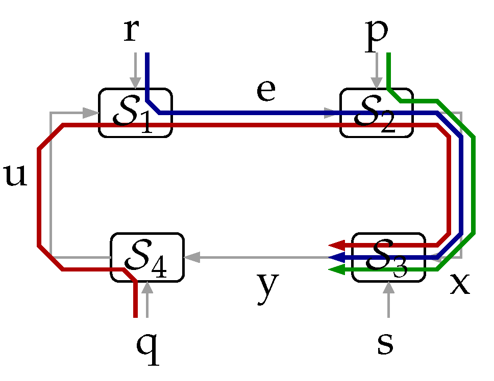
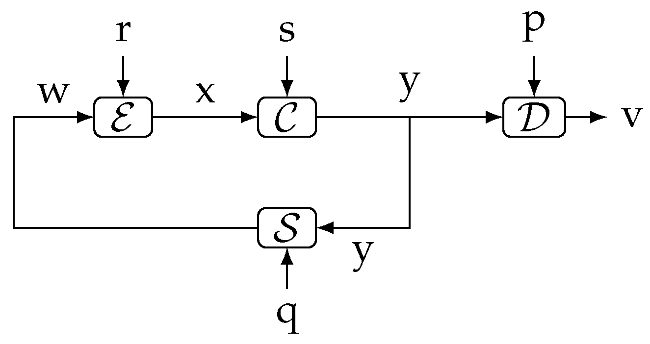
- Our first main contribution is the following theorem. It states a fundamental result, which relates the directed information between two signals within a feedback loop, say x and y, to the mutual information between an external set of signals and y:Theorem 1.The proof is in Section 3. This fundamental result, which for the cases in which can be understood as a law of conservation of information flow, is illustrated in Figure 2. (Here, and in the sequel, we use the notation to mean “x is independent of y”.) For such a cases, the information causally conveyed from x to y equals the information flow from to y. When are not independent of s, part of the mutual information between and y (corresponding to the term ) can be thought of as being “leaked” through s, thus bypassing the forward link from x to y. This provides an intuitive interpretation for (5).Figure 2. The flow of information between exogenous signals and the internal signal y equals the directed information from to when .Figure 2. The flow of information between exogenous signals and the internal signal y equals the directed information from to when .
![Entropy 23 00533 g002]() Remark 1.Theorem 1 implies that is only a part of (or at most equal to) the information “flow” between all the exogenous signals entering the loop outside the link (namely ), and y. In particular, if were deterministic, then , regardless of the blocks and irrespective of the nature of s.
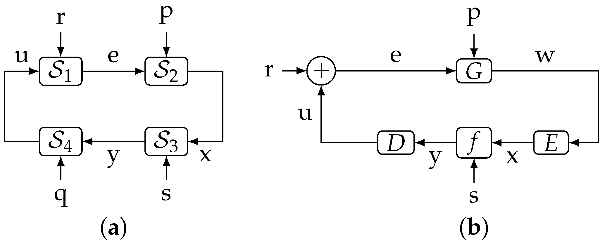
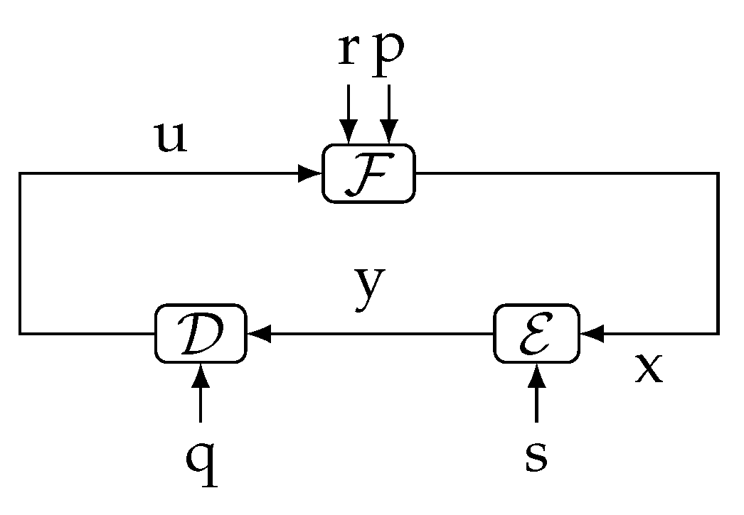
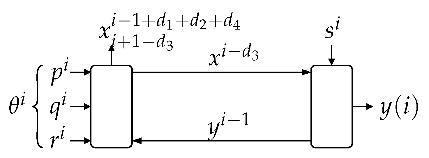
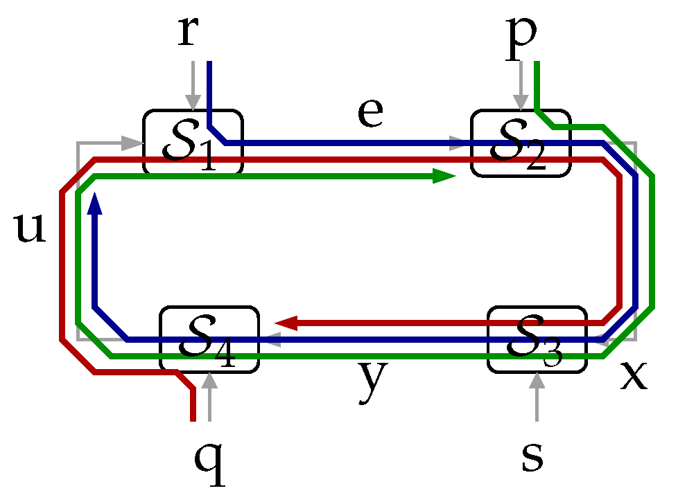
Remark 1.Theorem 1 implies that is only a part of (or at most equal to) the information “flow” between all the exogenous signals entering the loop outside the link (namely ), and y. In particular, if were deterministic, then , regardless of the blocks and irrespective of the nature of s. - Our second main result is the following theorem, which relates directed information involving four different sequences internal to the loop. The proof is in Appendix A on page 19.Theorem 2(Full Closed-Loop Directed Data-Processing Inequality). Consider the system shown in Figure 1a.
- (a)
- If and , or if and , then:
- (b)
- If and for , then:
(The Markov chain notation means “t and w are independent when v is given”.) To the best of our knowledge, Theorem 2 is the first result available in the literature providing a lower bound to the gap between two instances of nested directed information, involving four different signals inside the feedback loop. This result can be seen as the first full extension of the open-loop (traditional) data-processing inequality, to arbitrary closed-loop scenarios. (Notice that there is no need to consider systems with more than four mappings, since all external signals entering the loop between a given pair of internal signals can be regarded as exogenous inputs to a single equivalent deterministic mapping.) - Our third main contribution is introducing the notion of in-the-loop (ITL) transmission rate (in Section 6) for the (seldom considered) channel-coding scenario in which the messages to be transmitted and the communication channel are internal to a feedback loop. We show that the supremum of the directed information rate across such a channel upper bounds the achievable ITL transmission rates. Moreover, we present an example in which this upper bound is attainable. This gives further operational meaning to the directed information rate in closed-loop scenarios.
- Finally, we provide additional examples of the applicability of our results by discussing how they allow one to obtain the generalizations of two fundamental inequalities known in networked control literature. The first one appears in [18] (Lemma 4.1) and is written in (12) below. This generalization is a consequence of Theorem 4 and is discussed in Remarks 3 and 5 below. The second generalization applies to [20] (Theorem 4.1) and is described on page 6 below. It is an application of Theorem 2 that has just been carried out by the authors in [26], which is all the more important since, as we also reveal in that note, there is a flaw in the proof of [20] (Theorem 4.1).

1.2. Existing Related Results

1.3. Outline of the Paper
2. Preliminaries
2.1. Notation
2.2. Mutual Information
2.3. System Description
2.4. A Necessary Modification of the Definition of Directed Information
2.5. A Fundamental Lemma

3. Proof of Theorem 1
4. Relationships between Mutual and Directed Information
5. Relationships between Nested Directed Information
6. Giving Operational Meaning to the Directed Information: In-the-Loop Channel Coding
- If the feedback channel is deterministic, then is a deterministic function of and thus , as desired.
- If the (forward) communication channel is noiseless, then at each time , we have . Therefore . Again, if the feedback channel is deterministic, the ITL transmission rate is zero.
- In the absence of feedback, , recovering the notion of transmission rate of the case in which the messages are exogenous to the loop.
7. Concluding Remarks
- (1)
- Establishing whether (and under which conditions, if any) in the system of Figure 1, each of the following inequalities is true or false:
- (2)
- Extending Theorems 1 and 2 to scenarios with more than one feedback loop.
- (3)
- Exploring if tree codes [43] can be tailored to maximize the ITL data rate instead of the conventional data rate within a feedback loop. If such adaptation is possible, it would be interesting to assess how close to the ITL channel capacity such codes can perform.
Author Contributions
Funding
Institutional Review Board Statement
Informed Consent Statement
Conflicts of Interest
Appendix A. Proofs
References
- Cover, T.M.; Thomas, J.A. Elements of Information Theory, 2nd ed.; Wiley-Interscience: Hoboken, NJ, USA, 2006. [Google Scholar]
- Salek, S.; Cadamuro, D.; Kammerlander, P.; Wiesner, K. Quantum Rate-Distortion Coding of Relevant Information. IEEE Trans. Inf. Theory 2019, 65, 2603–2613. [Google Scholar] [CrossRef] [Green Version]
- Lindenstrauss, E.; Tsukamoto, M. From Rate Distortion Theory to Metric Mean Dimension: Variational Principle. IEEE Trans. Inf. Theory 2018, 64, 3590–3609. [Google Scholar] [CrossRef] [Green Version]
- Yang, Y.; Grover, P.; Kar, S. Rate Distortion for Lossy In-Network Linear Function Computation and Consensus: Distortion Accumulation and Sequential Reverse Water-Filling. IEEE Trans. Inf. Theory 2017, 63, 5179–5206. [Google Scholar] [CrossRef]
- Derpich, M.S.; Østergaard, J. Improved upper bounds to the causal quadratic rate-distortion function for Gaussian stationary sources. IEEE Trans. Inf. Theory 2012, 58, 3131–3152. [Google Scholar] [CrossRef] [Green Version]
- Ramakrishnan, N.; Iten, R.; Scholz, V.B.; Berta, M. Computing Quantum Channel Capacities. IEEE Trans. Inf. Theory 2021, 67, 946–960. [Google Scholar] [CrossRef]
- Song, J.; Zhang, Q.; Kadhe, S.; Bakshi, M.; Jaggi, S. Stealthy Communication Over Adversarially Jammed Multipath Networks. IEEE Trans. Inf. Theory 2020, 68, 7473–7484. [Google Scholar] [CrossRef]
- Makur, A. Coding Theorems for Noisy Permutation Channels. IEEE Trans. Inf. Theory 2020, 66, 6723–6748. [Google Scholar] [CrossRef]
- Kostina, V.; Verdú, S. Lossy joint source-channel coding in the finite blocklength regime. IEEE Trans. Inf. Theory 2013, 59, 2545–2575. [Google Scholar] [CrossRef] [Green Version]
- Huang, Y.; Narayanan, K.R. Joint Source-Channel Coding with Correlated Interference. IEEE Trans. Commun. 2012, 60, 1315–1327. [Google Scholar] [CrossRef] [Green Version]
- Steinberg, Y.; Merhav, N. On hierarchical joint source-channel coding with degraded side information. IEEE Trans. Inf. Theory 2006, 52, 886–903. [Google Scholar] [CrossRef]
- Hollands, S. Trace- and improved data processing inequalities for von Neumann algebras. arXiv 2021, arXiv:2102.07479. [Google Scholar]
- Massey, J.L. Causality, feedback and directed information. In Proceedings of the International Symposium on Information Theory and Its Applications, Honolulu, HI, USA, 27–30 November 1990; pp. 303–305. [Google Scholar]
- Kramer, G. Directed Information for Channels with Feedback. Ph.D. Thesis, Swiss Federal Institute of Technology, Zürich, Switzerland, 1998. [Google Scholar]
- Tatikonda, S.; Mitter, S. The Capacity of Channels With Feedback. IEEE Trans. Inf. Theory 2009, 55, 323–349. [Google Scholar] [CrossRef]
- Li, C.; Elia, N. The Information Flow and Capacity of Channels with Noisy Feedback. arXiv 2011, arXiv:1108.2815. [Google Scholar]
- Tatikonda, S.C. Control Under Communication Constraints. Ph.D. Thesis, Department of Electrical Engineering and Computer Science, Massachusetts Institute of Technology, Cambridge, MA, USA, 2000. [Google Scholar]
- Martins, N.C.; Dahleh, M.A. Fundamental limitations of performance in the presence of finite capacity feedback. In Proceedings of the 2005 American Control Conference, Portland, OR, USA, 8–10 June 2005. [Google Scholar]
- Martins, N.; Dahleh, M. Feedback control in the presence of noisy Channels: “Bode-like” fundamental limitations of performance. IEEE Trans. Autom. Control 2008, 53, 1604–1615. [Google Scholar] [CrossRef]
- Silva, E.I.; Derpich, M.S.; Østergaard, J. A framework for control system design subject to average data-rate constraints. IEEE Trans. Autom. Control 2011, 56, 1886–1899. [Google Scholar] [CrossRef] [Green Version]
- Silva, E.I.; Derpich, M.S.; Østergaard, J. On the Minimal Average Data-Rate That Guarantees a Given Closed Loop Performance Level. In Proceedings of the 2nd IFAC Workshop on Distributed Estimation and Control in Networked Systems, NECSYS, Annecy, France, 13–14 September 2010; pp. 67–72. [Google Scholar]
- Silva, E.I.; Derpich, M.S.; Østergaard, J. An achievable data-rate region subject to a stationary performance constraint for LTI plants. IEEE Trans. Autom. Control 2011, 56, 1968–1973. [Google Scholar] [CrossRef] [Green Version]
- Tanaka, T.; Esfahani, P.M.; Mitter, S.K. LQG Control With Minimum Directed Information: Semidefinite Programming Approach. IEEE Trans. Autom. Control 2018, 63, 37–52. [Google Scholar] [CrossRef] [Green Version]
- Quinn, C.; Coleman, T.; Kiyavash, N.; Hatsopoulos, N. Estimating the directed information to infer causal relationships in ensemble neural spike train recordings. J. Comput. Neurosci. 2011, 30, 17–44. [Google Scholar] [CrossRef]
- Permuter, H.H.; Kim, Y.H.; Weissman, T. Interpretations of directed information in portfolio theory, data Compression, and hypothesis testing. IEEE Trans. Inf. Theory 2011, 57, 3248–3259. [Google Scholar] [CrossRef]
- Derpich, M.S.; Østergaard, J. Comments on “A Framework for Control System Design Subject to Average Data-Rate Constraints”. arXiv 2021, arXiv:2103.12897. [Google Scholar]
- Massey, J.; Massey, P. Conservation of mutual and directed information. In Proceedings of the Proceedings. International Symposium on Information Theory, 2005. ISIT 2005, Adelaide, SA, Australia, 4–9 September 2005; pp. 157–158. [Google Scholar] [CrossRef]
- Kim, Y.H.; Kim, Y.H. A Coding Theorem for a Class of Stationary Channels With Feedback. IEEE Trans. Inf. Theory 2008, 54, 1488–1499. [Google Scholar] [CrossRef]
- Zamir, R.; Kochman, Y.; Erez, U. Achieving the Gaussian rate-distortion function by prediction. IEEE Trans. Inf. Theory 2008, 54, 3354–3364. [Google Scholar] [CrossRef]
- Zhang, H.; Sun, Y.X. Directed information and mutual information in linear feedback tracking systems. In Proceedings of the 6-th World Congress on Intelligent Control and Automation, Dalian, China, 21–23 June 2006; pp. 723–727. [Google Scholar]
- Silva, E.I.; Derpich, M.S.; Østergaard, J.; Encina, M.A. A characterization of the minimal average data rate that guarantees a given closed-lop performance level. IEEE Trans. Autom. Control 2016, 61, 2171–2186. [Google Scholar] [CrossRef]
- Derpich, M.S.; Silva, E.I.; Østergaard, J. Fundamental Inequalities and Identities Involving Mutual and Directed Informations in Closed-Loop Systems. arXiv 2013, arXiv:1301.6427. [Google Scholar]
- Shahsavari Baboukani, P.; Graversen, C.; Alickovic, E.; Østergaard, J. Estimating Conditional Transfer Entropy in Time Series Using Mutual Information and Nonlinear Prediction. Entropy 2020, 22, 1124. [Google Scholar] [CrossRef] [PubMed]
- Barforooshan, M.; Derpich, M.S.; Stavrou, P.A.; Ostergaard, J. The Effect of Time Delay on the Average Data Rate and Performance in Networked Control Systems. IEEE Trans. Autom. Control 2020, 1. [Google Scholar] [CrossRef]
- Baboukani, P.S.; Graversen, C.; Østergaard, J. Estimation of Directed Dependencies in Time Series Using Conditional Mutual Information and Non-linear Prediction. In Proceedings of the 2020 28th European Signal Processing Conference (EUSIPCO), Amsterdam, The Netherlands, 18–21 January 2021; pp. 2388–2392. [Google Scholar] [CrossRef]
- Yeh, J. Real Analysis, 3rd ed.; World Scientific: Singapore, 2014. [Google Scholar]
- Gray, R.M. Entropy and Information Theory, 2nd ed.; Science+Business Media, Springer: New York, NY, USA, 2011. [Google Scholar]
- Gray, R.M. Probability, Random Processes and Ergodic Properties, 2nd ed.; Springer: Berlin/Heidelberg, Germany, 2009. [Google Scholar]
- Yeung, R.W. A First Course in Information Theory; Springer: Berlin/Heidelberg, Germany, 2002. [Google Scholar]
- Goodwin, G.C.; Graebe, S.; Salgado, M.E. Control System Design; Prentice Hall: Hoboken, NJ, USA, 2001. [Google Scholar]
- Sahai, A.; Mitter, S. The Necessity and Sufficiency of Anytime Capacity for Stabilization of a Linear System Over a Noisy Communication Link–Part I: Scalar Systems. IEEE Trans. Inf. Theory 2006, 52, 3369–3395. [Google Scholar] [CrossRef]
- Khina, A.; Gårding, E.R.; Pettersson, G.M.; Kostina, V.; Hassibi, B. Control Over Gaussian Channels With and Without Source?Channel Separation. IEEE Trans. Autom. Control 2019, 64, 3690–3705. [Google Scholar] [CrossRef]
- Khina, A.; Halbawi, W.; Hassibi, B. (Almost) practical tree codes. In Proceedings of the 2016 IEEE International Symposium on Information Theory, Barcelona, Spain, 10–15 July 2016; pp. 2404–2408. [Google Scholar] [CrossRef] [Green Version]


Publisher’s Note: MDPI stays neutral with regard to jurisdictional claims in published maps and institutional affiliations. |
© 2021 by the authors. Licensee MDPI, Basel, Switzerland. This article is an open access article distributed under the terms and conditions of the Creative Commons Attribution (CC BY) license (https://creativecommons.org/licenses/by/4.0/).
Share and Cite
Derpich, M.S.; Østergaard, J. Directed Data-Processing Inequalities for Systems with Feedback. Entropy 2021, 23, 533. https://doi.org/10.3390/e23050533
Derpich MS, Østergaard J. Directed Data-Processing Inequalities for Systems with Feedback. Entropy. 2021; 23(5):533. https://doi.org/10.3390/e23050533
Chicago/Turabian StyleDerpich, Milan S., and Jan Østergaard. 2021. "Directed Data-Processing Inequalities for Systems with Feedback" Entropy 23, no. 5: 533. https://doi.org/10.3390/e23050533