Thermodynamic Definitions of Temperature and Kappa and Introduction of the Entropy Defect

Abstract

This paper develops explicit and consistent definitions of the independent thermodynamic properties of temperature and the kappa index within the framework of nonextensive statistical mechanics and shows their connection with the formalism of kappa distributions. By defining the “entropy defect” in the composition of a system, we show how the nonextensive entropy of systems with correlations differs from the sum of the entropies of their constituents of these systems. A system is composed extensively when its elementary subsystems are independent, interacting with no correlations; this leads to an extensive system entropy, which is simply the sum of the subsystem entropies. In contrast, a system is composed nonextensively when its elementary subsystems are connected through long-range interactions that produce correlations. This leads to an entropy defect that quantifies the missing entropy, analogous to the mass defect that quantifies the mass (energy) associated with assembling subatomic particles. We develop thermodynamic definitions of kappa and temperature that connect with the corresponding kinetic definitions originated from kappa distributions. Finally, we show that the entropy of a system, composed by a number of subsystems with correlations, is determined using both discrete and continuous descriptions, and find: (i) the resulted entropic form expressed in terms of thermodynamic parameters; (ii) an optimal relationship between kappa and temperature; and (iii) the correlation coefficient to be inversely proportional to the temperature logarithm.

1. Introduction

The existence of generalized thermal equilibrium requires the system to be residing in stationary states, i.e., where the (time independent) thermodynamic parameters, such as the temperature and the entropic index, can be well-defined.

Let two arbitrary and initially independent systems A and B interact through a wall permeable to heat transfer, eventually reaching (the generalized) thermal equilibrium. This is a stationary thermodynamic state, where no exchange of energy or entropy is observed [1,2,3], following:

$$\frac{1}{1-\frac{1}{\kappa }{S}_{\mathrm{A}}}\cdot \frac{\partial S_{\mathrm{A}}}{\partial U_{\mathrm{A}}}=\frac{1}{1-\frac{1}{\kappa }{S}_{\mathrm{B}}}\cdot \frac{\partial S_{\mathrm{B}}}{\partial U_{\mathrm{B}}},$$

(1)

and

$$S_{\mathrm{A}+\mathrm{B}}=S_{\mathrm{A}}+S_{\mathrm{B}}-\frac{1}{\kappa }{S}_{\mathrm{A}}{S}_{\mathrm{B}},$$

(2)

where we note that (i) the above equations provide, respectively, (a) a generalized thermodynamic definition of temperature (e.g., [1,3,4,5,6,7]), and (b) a partition expression of the entropy (e.g., [8,9]); (ii) the kappa index that parameterizes the formulation of kappa distributions was shown to be equivalent to the notation of the q-index that parameterizes the formulations of nonextensive statistical mechanics, under the transformation of their indices κ = 1/(q − 1) (e.g., see: [5]); and (iii) the Boltzmann constant k_B is set to 1 throughout the paper.

The temperature is defined through the change of entropy S, which is caused by a change of internal energy $U$; this is formally expressed through the invariant form shown in Equation (1).

$$\frac{1}{T}\equiv \frac{1}{1-\frac{1}{\kappa }S}\cdot \frac{\partial S}{\partial U}.$$

(3)

This recovers the classical thermal equilibrium and the Clausius related formulation for κ→∞, that is, $1/T\equiv \partial S/\partial U$ [10] (see also: [11,12]. Note: canonical ensemble, the volume, and number of particles of the system is constant, i.e., $\partial S/\partial U$ means ${(\partial S/\partial U)}_{V,N}$).

The entropy partitioning rule of Equation (2) describes a special type of entropy composability; the latter means that the entropy of the total system, which is composed of independent subsystems, can be given as a function of the entropies of the subsystems [13], i.e., $S_{\mathrm{A}+\mathrm{B}}=f(S_{\mathrm{A}},S_{\mathrm{B}})$ (see also: [14,15]). This exact form is sometimes called the pseudo-additivity rule because it generalizes the classical entropy additivity rule, that is, $S_{\mathrm{A}+\mathrm{B}}=S_{\mathrm{A}}+S_{\mathrm{B}}$, which it recovers for κ→∞. Apparently, for systems with correlations this rule does not generally apply, while for special types of correlations it is possible that the additivity may be recovered (e.g., [16,17]).

It has been shown that the pseudo-additivity rule is equivalent to the Tsallis entropy and to the formulation of kappa distributions: First, we recall that Tsallis entropy [18,19,20]) is equivalent to the formulation of kappa distributions (e.g., [5,21,22,23,24]; see also: [25,26,27] and [28,29,30,31,32,33,34,35,36]); indeed, this entropic formulation is maximized under the constraints of canonical ensemble leading to kappa distributions [5], and vice versa, when maximized, the entropic formulation leads to the specific form of kappa distributions [37,38]. Then, it can be easily shown that the Tsallis entropic function obeys to the pseudo-additivity rule [18]. Alternatively, when starting from the pseudo-additivity rule, the entropic function obeying this rule is the Tsallis entropy [3,8,39,40].

The pseudo-additivity rule provides the thermodynamic definition of kappa:

$$\frac{1}{\kappa }\equiv \frac{(S_{\mathrm{A}}+S_{\mathrm{B}})-S_{\mathrm{A}+\mathrm{B}}}{S_{\mathrm{A}}{S}_{\mathrm{B}}},$$

(4)

which provides a measure of the loss (for κ > 0) or gain (for κ < 0) of entropy after mixing partial systems A and B to compose the combined system.

The expressions in Equations (3) and (4) are stated as the thermodynamic definitions of temperature and kappa, respectively. However, they involve several physical inconsistencies, which we resolve in this paper:

(i)

The thermodynamic definition of the temperature is not well-stated since it involves also another independent thermodynamic parameter, the kappa index.

(ii)

There is no clear connection between entropic loss and kappa for any individual or composed system, and the same holds for the thermodynamic definition of the kappa.

(iii)

There is not an obvious connection with the formalism of kappa distributions and the corresponding kinetic definitions of temperature and kappa index.

(iv)

There is no well-determined formulation for the entropy of a combined system with correlations between its subsystems.

The purpose of this paper is to develop explicit thermodynamic definitions of temperature and the kappa index and show their connection with the formalism of nonextensive statistical mechanics and kappa distributions. In Section 2, we interpret the entropy variations that have occurred along the composition of a system; in particular, we define the concept of an “entropy defect” and develop the composition of a system in both discrete and continuous descriptions. We also show the connection of nonextensive entropy characterized by an entropy defect, with the formalism of kappa distributions. In Section 3, we provide consistent thermodynamic definitions of the kappa index and temperature and show their connection with the respective kinetic definitions. In Section 4, we derive the complete formulation of nonextensive entropy in terms of temperature, in both the discrete and continuous descriptions, and show how this form is associated with kappa distributions. In Section 5, we express the nonextensive entropy defect of a system composed by a number of subsystems with correlations in terms of temperature. By maximizing this entropy defect, we also determine a relationship between the independent thermodynamic parameters of kappa and temperature. Finally, Section 6 summarizes and provides the conclusions, while in the Appendix A we provide the basic derived expressions in terms of the entropic q-index.

2. Entropic Composition of a System

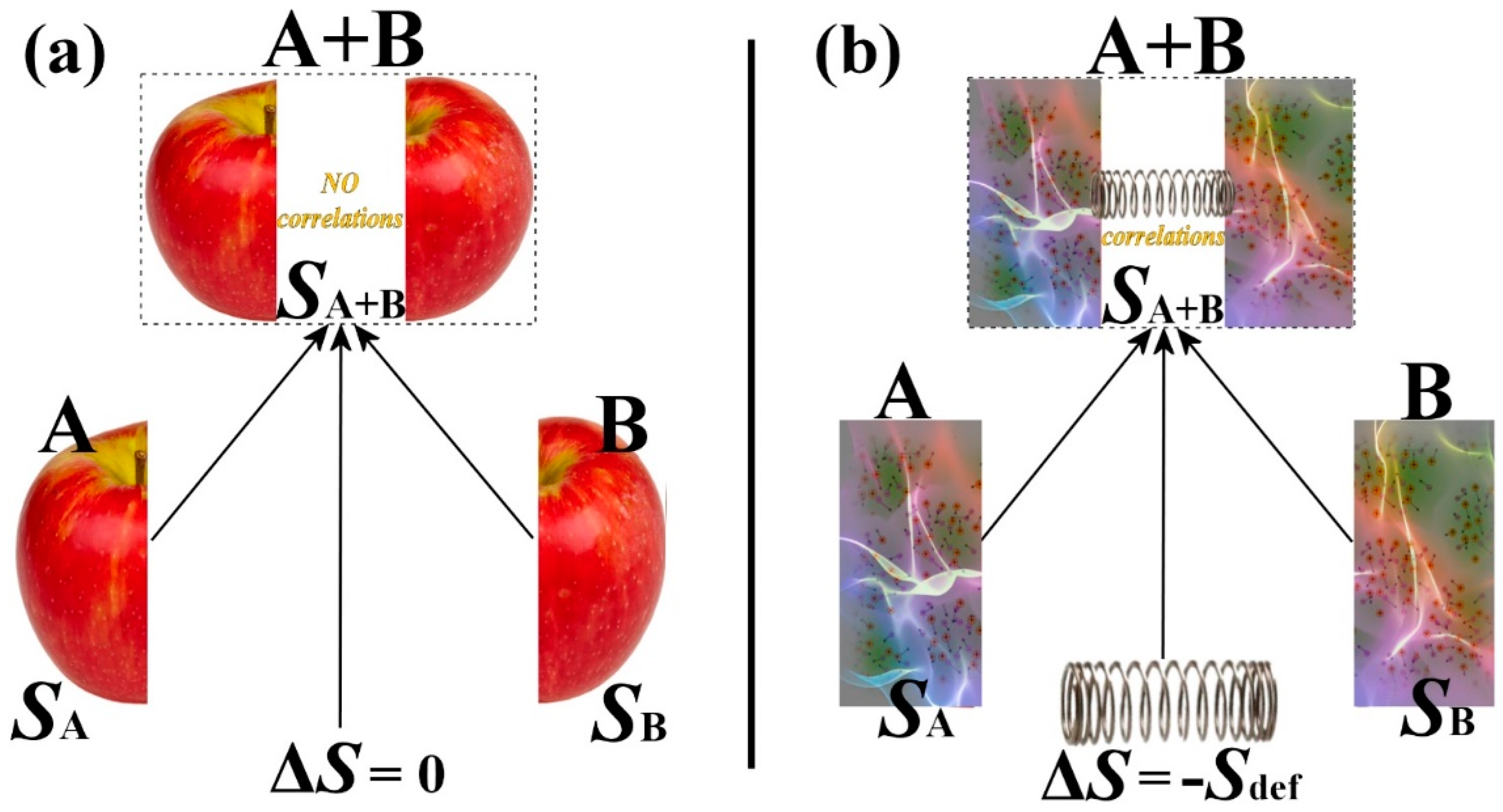
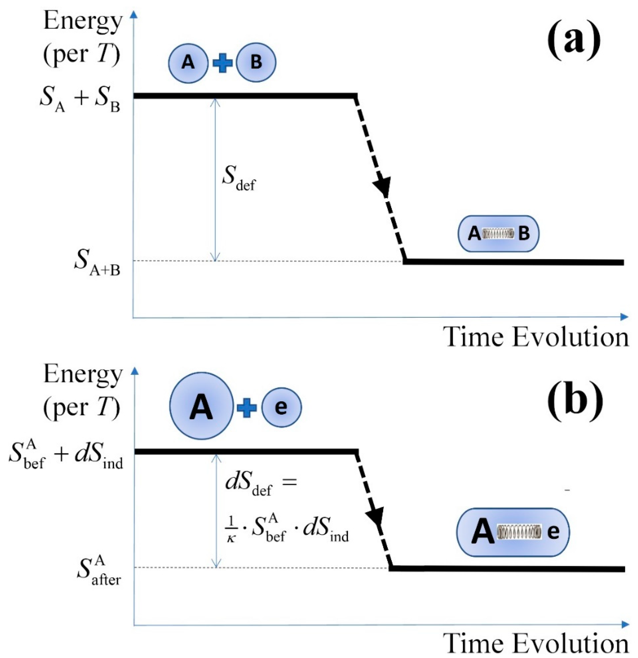
2.1. Entropy Defect

While the composition of two, originally independent, subsystems A and B into the combined system A+B is generally completed through an irreversible mixing thermodynamic process, it can be approached by a progressive series of slow quasi-stationary and quasi-reversible (called quasistatic) processes, for which the entropy is additive (e.g., [41,42]). At each procedure, a small portion of entropy dS is moved from each partial system to the total, $d{S}_{\mathrm{A}+\mathrm{B}}\approx d{S}_{\mathrm{A}}+d{S}_{\mathrm{B}}$, until the completion of all the mixing procedures, obtaining $S_{\mathrm{A}+\mathrm{B}}\approx S_{\mathrm{A}}+S_{\mathrm{B}}$.

In this classical approach, there is no consideration of the entropy associated with correlations induced by long-range interactions acting among the particles. When A and B were separated, there was no interaction or correlation between them. Once they are mixed into a combined system characterized by such interactions that can produce correlations (e.g., long-range interactions), then order is added to the system, and thus its entropy decreases. If the long-range interactions and the induced correlations could have somehow disappeared, then an equal amount of entropy would have been added and consumed by the disorder generated by the resolution of these correlations. Measuring the initial S_A, S_B, and final S_A+B entropies, one may find the missing entropy due to the correlations, S_A + S_B – S_A+B. We interpret this missing entropy as an “entropy defect” S_def, that is, the portion of entropy by which the total entropy decreases the sum of entropies of the combined system due to the order generated by the correlations. This amount of entropy can be released at the composition of the system from its constituents. (Note: hereafter, we will refer to the constituents that compose the whole system, which can be either smaller subsystems of particles or individual particles.)

As illustrated in Figure 1, the entropy defect is a consequence of the presence of correlations among the constituents of systems. The connection of two subsystems with short-range interactions is not characterized by correlations and thus does not have an entropy defect. On the contrary, the connection of two subsystems with long-range interactions characterized by correlations requires an entropy defect expressed by Equation (5), shown below, which is also consistent with thermodynamics [3].

Thus, we write:

$$S_{\mathrm{A}+\mathrm{B}}=S_{\mathrm{A}}+S_{\mathrm{B}}-S_{\mathrm{def}}(S_{\mathrm{A}},S_{\mathrm{B}}).$$

(5)

The simplest construction of the nonadditive and nonlinear term causing the entropic defect would simply be proportional to the initial entropies S_A and S_B, i.e.,

$$S_{\mathrm{def}}(S_{\mathrm{A}},S_{\mathrm{B}})=\frac{1}{\kappa }\cdot S_{\mathrm{A}}\cdot S_{\mathrm{B}}.$$

(6)

In fact, this exact formulation, which leads to the entropy partitioning of Equation (2), was shown that can be derived by only assuming the existence of a thermodynamic stationary state, that is, a generalized thermal equilibrium [3]. The constant proportionality term 1/κ provides an independent thermodynamic parameter, that is, the kappa index κ, (Equation (4)). (In Section 4, we will discuss further the direct connection of correlations with the kappa index, using the findings of [43].)

2.2. Composition of a System: Discrete and Continuous Ways

Let the system of entropy S be constructed by combining N independent elementary subsystems, each of entropy dS_ind. The mixing includes long-range interactions that induce correlations among the subsystems; therefore, there is an entropy defect, dS_def, associated with a kappa index, κ. Then, the elementary subsystem interacts and merges with the particle system, changing the entropy of the latter as follows:

$$S_{\mathrm{after}}=S_{\mathrm{bef}}+d{S}_{\mathrm{ind}}-d{S}_{\mathrm{def}}(S_{\mathrm{bef}},d{S}_{\mathrm{ind}}),$$

(7)

with

$$d{S}_{\mathrm{def}}(S_{\mathrm{bef}},d{S}_{\mathrm{ind}})=\frac{1}{\kappa }d{S}_{\mathrm{ind}}\cdot S_{\mathrm{bef}}.$$

(8)

The collection of a number of n independent elementary subsystems can be seen as a classical (extensive) system, without any correlations among the subsystems, whose total entropy is given by:

$$S_{\mathrm{ind}}{}_n=n\cdot d{S}_{\mathrm{ind}}.$$

(9)

On the other hand, the collection of the n independent elementary subsystems within the (nonextensive) system of entropy S, characterized by correlations and thus an entropy defect, is obviously not given by its extensive expression (9). In order to derive the entropy of the system S as a function of the elementary element entropy dS_ind, we first need to understand the construction of the system; this can be interpreted either within the continuous or discrete framework. The discrete description follows Equations (7) and (8), which can be written after some calculus:

$$S_{\mathrm{after}}=(1-\frac{1}{\kappa }d{S}_{\mathrm{ind}})\cdot S_{\mathrm{bef}}+d{S}_{\mathrm{ind}}.$$

(10)

For the continuous description, we substitute in (5), as follows: the elementary subsystem of infinitesimal entropy dS_ind interacts with the system of entropy S; hence, $S_{\mathrm{A}}=S$, $S_{\mathrm{B}}=d{S}_{\mathrm{ind}}$ (before) and $S_{\mathrm{A}+\mathrm{B}}=S+dS$ (after). The entropic change of the system, dS, is caused by the elementary subsystem entropies and the entropy defect, i.e.,

$$dS=(1-\frac{1}{\kappa }S)\cdot d{S}_{\mathrm{ind}},$$

(11)

or

$$dS=d{S}_{\mathrm{ind}}-d{S}_{\mathrm{def}}\mathrm{with}d{S}_{\mathrm{def}}=\frac{1}{\kappa }\cdot S\cdot d{S}_{\mathrm{ind}}.$$

(12)

Equations (10) and (11) express the composition (and decomposition) of a system, by means of its entropy, in a discrete and continuous description, respectively. Both formalisms become trivial in the classical case of no entropy defect, leading into simple additions, i.e., $S_{\mathrm{after}}=S_{\mathrm{bef}}+d{S}_{\mathrm{ind}}$ and $dS=d{S}_{\mathrm{ind}}$.

Figure 2 illustrates the entropy defect in the total entropy of a system, when (a) it is composed by two subsystems A and B, as shown in Equations (5) and (6), and (b) an independent elementary subsystem is added to it, as shown in Equations (7) and (8).

Next, we solve Equations (10) and (11) to express the total nonextensive entropy S of a composed system, when this is constructed in the presence of correlations among its constituents. This entropy is expressed in terms of its extensive limit, S_ind, that is, the entropy of the collection of all the elementary subsystems, which would have been the actual entropy S of the system if there were no correlations.

2.3. Connection with the Formalism of Kappa Distributions

2.3.1. General

Here, we develop and solve the (difference/differential) equations of entropy that provide the total nonextensive entropy of the system S, expressed in terms of its extensive limit, S_ind. We examine both the discrete and continuous descriptions and show that the formalism of kappa distributions appears naturally in the expression of the nonextensive entropy.

2.3.2. Discrete Description

Equation (10) constitutes a 1D linear discrete map or difference equation (e.g., [6,44,45,46]), which can be solved to find the entropy S_n for each n:

$$S_n=(1-\frac{1}{\kappa }d{S}_{\mathrm{ind}})\cdot S_{n-1}+d{S}_{\mathrm{ind}},\mathrm{for}\mathrm{all}n=1,2,\dots ,N.$$

(13)

It describes the entropy S_n of a system, which is composed nonextensively of n elementary subsystems, each of entropy dS_ind, when constructed by the interaction of a system with entropy S_n−1 (composed nonextensively of n−1 elementary subsystems) and a single elementary subsystem. Equation (13) can be rewritten as:

$$(1-\frac{1}{\kappa }{S}_n)=(1-\frac{1}{\kappa }d{S}_{\mathrm{ind}})\cdot (1-\frac{1}{\kappa }{S}_{n-1}),\mathrm{for}\mathrm{all}n=1,2,\dots ,N.$$

(14)

We set $x_n\equiv 1-\frac{1}{\kappa }{S}_n$ and $\alpha \equiv 1-\frac{1}{\kappa }d{S}_{\mathrm{ind}}$, and thus Equation (14) is written as $x_n=\alpha \cdot x_{n-1}={\alpha }^2\cdot x_{n-2}$$={\alpha }^n\cdot x_0$, where $x_0\equiv 1-\frac{1}{\kappa }{S}_0=1$, since there is no initial system and no entropy ($S_0=0$) existing before the very first mixing of elementary subsystems. Hence, $(1-\frac{1}{\kappa }{S}_n)={(1-\frac{1}{\kappa }d{S}_{\mathrm{ind}})}^n$, or given of Equation (9),

$$(1-\frac{1}{\kappa }{S}_n)={(1-\frac{1}{n\cdot \kappa }{S}_{\mathrm{ind}}{}_n)}^n,\mathrm{for}\mathrm{all}n=0,1,\dots ,N,$$

(15)

or

$${(1-\frac{1}{\kappa }{S}_n)}^{-\kappa }={(1-\frac{1}{n\cdot \kappa }{S}_{\mathrm{ind}}{}_n)}^{-n\cdot \kappa },\mathrm{for}\mathrm{all}n=0,1,\dots ,N.$$

(16)

Therefore, from Equation (15) we find that for a final number of N elementary subsystems involved in the final composed system, we have:

$${(1-\frac{1}{\kappa }{S}_N)}^{-\kappa }={(1-\frac{1}{N\cdot \kappa }{S}_{\mathrm{ind}}{}_N)}^{-N\cdot \kappa },$$

(17)

and thus, the entropy of the system is given by:

$$S_N=\kappa \cdot \left[1-{(1-\frac{1}{N\cdot \kappa }{S}_{\mathrm{ind}}{}_N)}^N\right].$$

(18)

We also recall the known notation of deformed exponential/logarithm functions:

$$W\equiv {\exp }_{\kappa }(S_N)={\exp }_{(N\cdot \kappa )}(S_{\mathrm{ind}}{}_N),$$

(19)

which constitutes the multiplicity W (or statistical weight), that is, the number of microstates corresponding to a particular macrostate of a thermodynamic system. Then, we can solve in terms of entropies:

$$S_N={\ln }_{\kappa }\left[{\exp }_{(N\cdot \kappa )}(S_{\mathrm{ind}}{}_N)\right]\iff S_{\mathrm{ind}}{}_N={\ln }_{(N\cdot \kappa )}\left[{\exp }_{\kappa }(S_N)\right],$$

(20)

where the κ- deformed exponential function and its inverse, the deformed logarithm function (e.g., see: [47,48,49,50]),

$${\exp }_{\kappa }(x)\equiv {(1-\frac{1}{\kappa }x)}^{-\kappa },{\ln }_{\kappa }(x)\equiv \kappa (1-x^{-\frac{1}{\kappa }}),$$

(21)

with

$${\exp }_{\kappa }[{\ln }_{\kappa }(x)]={\ln }_{\kappa }[{\exp }_{\kappa }(x)]=x.$$

(22)

Here, we use the kappa index as a subscript for the notation of the deformed functions but note that the q-index could have been equivalently used (see also: Appendix A).

For a large number N of the involved elementary subsystems, N >> 1, and considering that the extensive entropy has a given fixed value, i.e., $d{S}_{\mathrm{ind}}{}_N=S_{\mathrm{ind}}{}_N/N$, we obtain:

$${(1-\frac{1}{N\cdot \kappa }{S}_{\mathrm{ind}}{}_N)}^{-N\cdot \kappa }\to \exp (S_{\mathrm{ind}}{}_N).$$

(23)

Hence, Equations (17)–(20) can be, respectively, reduced, for a large N, as:

$${(1-\frac{1}{\kappa }{S}_N)}^{-\kappa }=\exp (S_{\mathrm{ind}}{}_N),$$

(24)

$$S_N=\kappa \cdot (1-e^{-\frac{1}{\kappa }\cdot S_{\mathrm{ind}}{}_N}),$$

(25)

$$W={\exp }_{\kappa }(S_N)=\exp (S_{\mathrm{ind}}{}_N),$$

(26)

$$S_N={\ln }_{\kappa }\left[\exp (S_{\mathrm{ind}}{}_N)\right]\iff S_{\mathrm{ind}}{}_N=\ln \left[{\exp }_{\kappa }(S_N)\right],$$

(27)

where we observe that the multiplicity $W={\exp }_{\kappa }(S_N)$ becomes a thermodynamic quantity independent of the kappa index (see Figure 3). In addition, Equation (27) shows that a system, consisting of N elementary subsystems, has an entropy equal to S_{ind N} if the composition is constructed with no correlations (extensively) and entropy equal to S_N if the composition is constructed with correlations (nonextensively).

2.3.3. Continuous Description

Equation (11) can be solved directly, by integrating from Equation (11) the system’s entropy dS from 0 to S and elementary entropy dS_ind from 0 to S_ind, obtaining:

$${(1-\frac{1}{\kappa }S)}^{-\kappa }=\exp (S_{\mathrm{ind}}),$$

(28)

$$S=\kappa \cdot (1-e^{-\frac{1}{\kappa }\cdot S_{\mathrm{ind}}}),$$

(29)

$$W={\exp }_{\kappa }(S)=\exp (S_{\mathrm{ind}}),$$

(30)

$$S={\ln }_{\kappa }\left[\exp (S_{\mathrm{ind}})\right]\iff S_{\mathrm{ind}}=\ln \left[{\exp }_{\kappa }(S)\right],$$

(31)

which are similar to Equations (24)–(27), respectively, when interpreting the entropy of a collection of N subsystems in a continuous description, namely, $S_N\to S=S(N)$ and $S_{\mathrm{ind}}{}_N\to S_{\mathrm{ind}}=S_{\mathrm{ind}}(N)$. Equations (18) (discrete description) and (25) or (29) (continuous description) completed the task of expressing the total nonextensive entropy of the system S in terms of its extensive limit, S_ind.

It is also important that we produced the formalism of kappa distributions for the entropic form, starting only from thermodynamic definitions (compare with the entropic form for kappa distributions [3]). Section 4 will analyze further this result, expressing entropy in terms of both kappa and temperature.

3. Thermodynamic Definitions

3.1. Thermodynamic Definition of the Kappa Index

The entropy defect defines the kappa index within a thermodynamic context. Starting from Equation (8), which expresses the entropy defect of mixing a system of entropy S with an elementary independent subsystem of entropy S_ind,

$$d{S}_{\mathrm{def}}(S,d{S}_{\mathrm{ind}})=\frac{1}{\kappa }d{S}_{\mathrm{ind}}\cdot S,$$

(32)

we obtain the thermodynamic definition of the kappa:

$$\frac{1}{\kappa }\equiv \frac{d{S}_{\mathrm{def}}}{Sd{S}_{\mathrm{ind}}}.$$

(33)

We recall that we work in the framework of the canonical ensemble and fixed volume and number of particles. Hence, the involved derivatives are written as: $dS/d{S}_{\mathrm{ind}}\to {(\partial S/\partial S_{\mathrm{ind}})}_{V,N}$ and $\partial S/\partial U\to {(\partial S/\partial U)}_{V,N}$. Hence, the definition becomes:

$$\frac{1}{\kappa }\equiv \frac{1}{S}\cdot {\left(\frac{\partial S_{\mathrm{def}}}{\partial S_{\mathrm{ind}}}\right)}_{V,N}.$$

(34)

Thus, when adding an independent part of entropy dS_ind to a system with correlations among its constituents, its entropy S increases by a smaller amount, dS = dS_ind − dS_def, where the difference is caused by the corresponding entropy defect dS_def that determines the thermodynamic value of kappa according to Equation (34).

The ratio of the entropy defect per entropy of the elementary independent subsystems that compose the total system, normalized to the entropy of the system, constitutes the thermodynamic definition of the inverse kappa (with the appropriate care of the defect sign); note the similarity of the thermodynamic definition of the inverse temperature.

The thermodynamic definition is actually used to derive the connection between nonextensive and extensive entropies (as shown in Equation (11) and found in Equation (29)), namely:

$$\frac{1}{\kappa }=-\frac{(S+dS)-(S+d{S}_{\mathrm{ind}})}{Sd{S}_{\mathrm{ind}}}=\frac{1}{S}\cdot \left(1-\frac{dS}{d{S}_{\mathrm{ind}}}\right).$$

(35)

3.2. Thermodynamic Definition of the Temperature

Considering again the fixed volume and number of particles, Equation (11) becomes:

$$1-\frac{1}{\kappa }S={\left(\frac{\partial S}{\partial S_{\mathrm{ind}}}\right)}_{V,N},$$

(36)

while the thermodynamic definition of temperature, Equation (3), is written as:

$$\frac{1}{T}\equiv \frac{1}{1-\frac{1}{\kappa }S}\cdot {\left(\frac{\partial S}{\partial U}\right)}_{V,N}=\frac{{\left(\partial S/\partial U\right)}_{V,N}}{{\left(\partial S/\partial S_{\mathrm{ind}}\right)}_{V,N}}={\left(\frac{\partial S_{\mathrm{ind}}}{\partial U}\right)}_{V,N},$$

(37)

which is now expressed without involving of the independent thermodynamic property of the kappa index. Note that the expression connects the temperature with the extensive entropy of the system, corresponding to the collection of independent elementary subsystems. This matches the classical Clausius thermodynamic definition of temperature, where the entropy is extensive, $1/T\equiv {(\partial S/\partial U)}_{V,N}$.

We highlight the difference from the classical thermodynamic definition of temperature, which is the existence of the entropy defect, explicitly expressed in:

$$\frac{1}{T}\equiv {\left(\frac{\partial S_{\mathrm{ind}}}{\partial U}\right)}_{V,N}={\left(\frac{\partial S}{\partial U}\right)}_{V,N}+{\left(\frac{\partial S_{\mathrm{def}}}{\partial U}\right)}_{V,N}.$$

(38)

3.3. Connection with the Kinetic Definitions

The kinetic definition of the temperature and the kappa index are, respectively, related to the particle kinetic energy expectation value [5] and correlations [43,51,52]. In particular, the temperature is kinetically defined by the mean particle kinetic energy $\langle \epsilon \rangle$ per half degrees of freedom D, while the kappa index is kinetically defined by the correlation $\rho$ of the kinetic energies among any two particles (see also: [23], Chapter 5, and [53,54]). Accompanying the kinetic and thermodynamic definitions, we have for the kappa:

$$\frac{1}{\kappa }\equiv \frac{\rho }{\frac{1}{2}D},\frac{1}{\kappa }\equiv \frac{1}{S}\cdot {\left(\frac{\partial S_{\mathrm{def}}}{\partial S_{\mathrm{ind}}}\right)}_{V,N},$$

(39)

and the temperature:

$$\frac{1}{T}\equiv \frac{\frac{1}{2}D}{\langle \epsilon \rangle },\frac{1}{T}\equiv {\left(\frac{\partial S_{\mathrm{ind}}}{\partial U}\right)}_{V,N}.$$

(40)

An interesting combination of both definitions, canceling out the elementary entropy, is:

$$\frac{1}{\kappa T}\equiv \frac{\rho }{\langle \epsilon \rangle },\frac{1}{\kappa T}\equiv \frac{1}{S}\cdot {\left(\frac{\partial S_{\mathrm{def}}}{\partial U}\right)}_{V,N}.$$

(41)

Lastly, we can express directly the kinetic energy expectation value and correlation to the thermodynamic quantities:

$$\rho ~\frac{1}{S}\cdot {\left(\frac{\partial S_{\mathrm{def}}}{\partial S_{\mathrm{ind}}}\right)}_{V,N},\langle \epsilon \rangle ~{\left(\frac{\partial U}{\partial S_{\mathrm{ind}}}\right)}_{V,N},$$

(42)

with all entropies normalized to the half degrees of freedom (i.e., $S/(\frac{1}{2}D)\to S$). As expected, the particle kinetic energy expectation value and correlation are, respectively, proportional to the internal energy and entropy defect, per extensive entropy.

4. Entropic Formalism Associated with Kappa Distributions

In Section 2.3 and Equations (28)–(31), we derived the expression of the total nonextensive entropy of the system S in terms of its extensive limit, S_ind. Since S_ind refers to an extensive collection of the elementary subsystems, it is independent of the kappa index, expressed as a function of the temperature. Indeed, we have:

$$d{S}_{\mathrm{ind}}=dU/T=\frac{1}{2}D\cdot N\cdot dT/T=\frac{1}{2}D\cdot N\cdot d\ln (T/T_0),$$

(43)

or

$$S_{\mathrm{ind}}=\frac{1}{2}D\cdot N\cdot \ln (T/T_0),$$

(44)

where the thermal constant T₀ constitutes the minimum temperature for the entropy to be positive. In [55,56] and [23] (Chapters 2 and 5), this thermal constant was shown to be given by $k_{\mathrm{B}}{T}_0=C\cdot {\hslash }_{\mathrm{c}}^2{(m_{\mathrm{e}}{m}_{\mathrm{i}})}^{-\frac{1}{2}}\cdot {\mathsf{\lambda }}_{\mathrm{c}}^{-2}\cdot g_{\kappa ,N}$, where C = (9π/2)^1/3/e ≈ 0.89; λ_c is the smallest correlation length, which is interpreted by the interparticle distance b~n^−1/d for collisional particle systems (absence of correlations) or by the Debye length λ_D for collisionless particle systems (presence of local correlations) [57,58]. The factor g_κ,N depends on the kappa index κ and the number of correlated particles; for a large number of particles, it becomes g_κ,N ≈ 1. Finally, the phase-space parcel ${\hslash }_{\mathrm{c}}^{}$ is typically given by the Planck’s constant, but it was shown to represent a different and larger constant in space plasmas, where Debye shielding limits the distance of correlations, ${\hslash }_{*}^{}=(1.19\pm 0.05)\times {10}^{-22}\mathrm{J}\cdot \mathrm{s}$ [55,59,60,61,62,63] (namely, ${\hslash }_{\mathrm{c}}^{}$ = $\hslash$, when no correlations exist among particles, and ${\hslash }_{\mathrm{c}}^{}$ = ${\hslash }_{*}^{}$, when significant correlations exist among particles beyond their nearest neighbors, as in the case of the majority of space plasmas).

Combining now Equation (44), that is, the expression of the extensive entropy in terms of the temperature, S_ind (T), with Equation (18) or Equation (29), that is, the expression of the nonextensive S in terms of extensive S_ind entropies, we end up with the expression of the nonextensive entropy S in terms of the temperature, S (T).

For the discrete description, we obtain:

$${(1-\frac{1}{\kappa }{S}_N)}^{-\kappa }={(1-\frac{1}{N\cdot \kappa }{S}_{\mathrm{ind}}{}_N)}^{-N\cdot \kappa }={\left[1-\frac{\frac{1}{2}D}{\kappa }\ln (T/T_0)\right]}^{-N\cdot \kappa },$$

(45)

leading to

$$S_N=\kappa \cdot \left\{1-{\left[1-\frac{1}{\kappa }\cdot \frac{1}{2}D\cdot \ln (T/T_0)\right]}^N\right\}.$$

(46)

For the continuous description, we can write $d\ln {(T/T_0)}^{\frac{1}{2}D\cdot N}=d{S}_{\mathrm{ind}}=dS/(1-\frac{1}{\kappa }S)$$=d[\ln {(1-\frac{1}{\kappa }S)}^{-\kappa }]$ and obtain:

$${(1-\frac{1}{\kappa }S)}^{-\kappa }\equiv {\exp }_{\kappa }(S)=\exp (S_{\mathrm{ind}})={(T/T_0)}^{\frac{1}{2}D\cdot N},$$

(47)

leading to

$$S=\kappa \cdot \left(1-e^{-\frac{1}{\kappa }\cdot S_{\mathrm{ind}}}\right)=\kappa \cdot \left[1-{(T/T_0)}^{-\frac{1}{\kappa }\cdot \frac{1}{2}D\cdot N}\right],$$

(48)

or

$$S\equiv {\ln }_{\kappa }\left[\exp (S_{\mathrm{ind}})\right]={\ln }_{\kappa }\left[{(T/T_0)}^{\frac{1}{2}D\cdot N}\right].$$

(49)

Note that we may arrive at the continuous description and Equations (47) and (48), starting from the discrete description and Equations (45) and (46). Indeed, for N >> 1, and considering that the extensive entropy has a given fixed value, i.e., $S_{\mathrm{ind}}{}_N\ne S_{\mathrm{ind}}{}_N(N)$ and $d{S}_{\mathrm{ind}}{}_N=S_{\mathrm{ind}}{}_N/N$, we have ${\left\{1-\frac{1}{N}\cdot \left[\frac{1}{\kappa }\cdot \frac{1}{2}D\cdot N\cdot \ln (T/T_0)\right]\right\}}^N$→$\exp \left[-\frac{1}{\kappa }\cdot \frac{1}{2}D\cdot N\cdot \ln (T/T_0)\right]$$={(T/T_0)}^{-\frac{1}{\kappa }\cdot \frac{1}{2}D\cdot N}$.

We have ended up with the nonextensive entropy as a function of the independent thermodynamic properties of the kappa index and temperature. This temperature–entropy relationship is associated with kappa distributions and generalizes the Sackur–Tetrode entropic formula [64,65]. This is derived as follows. First, we substitute from Equations (46) and (48) the thermal constant T₀, defined in Equation (44) as $k_{\mathrm{B}}{T}_0=C\cdot {\hslash }_{\mathrm{c}}^2{(m_{\mathrm{e}}{m}_{\mathrm{i}})}^{-\frac{1}{2}}\cdot {\mathsf{\lambda }}_{\mathrm{c}}^{-2}\cdot g_{\kappa ,N}$, with $g_{\kappa ,N}\cong 1$, ${\mathsf{\lambda }}_{\mathrm{c}}^{}=b=n^{-\frac{1}{3}}$, ${\hslash }_{\mathrm{c}}^{}=\hslash$, and we find, respectively:

$$S_N(n,T,N,\kappa )=\kappa \cdot \left\{1-{\left\{1-\frac{1}{\kappa }\cdot \ln \left\{{\left[C\cdot k_{\mathrm{B}}^{-1}{\hslash }^2{(m_{\mathrm{e}}{m}_{\mathrm{i}})}^{-\frac{1}{2}}\right]}^{-\frac{3}{2}}\cdot \frac{T^{\frac{3}{2}}}{n}\right\}\right\}}^N\right\},$$

(50)

and

$$S(n,T,N,\kappa )=\kappa \cdot \left\{1-{\left\{{\left[C\cdot k_{\mathrm{B}}^{-1}{\hslash }^2{(m_{\mathrm{e}}{m}_{\mathrm{i}})}^{-\frac{1}{2}}\right]}^{-\frac{3}{2}}\cdot \frac{T^{\frac{3}{2}}}{n}\right\}}^{-\frac{1}{\kappa }\cdot N}\right\}.$$

(51)

Then, we express Equation (50) or Equation (51) in terms of the number of particles N, internal energy $U=\frac{3}{2}N\cdot k_{\mathrm{B}}T$, and volume $V=N/n$, following the steps shown in the direct derivation from kappa distributions in [3] (see also: [66]):

$$S_N(V,T,N,\kappa )=\kappa \cdot \left\{1-{\left\{1-\frac{1}{\kappa }\cdot \ln \left\{{\left[\frac{3}{2}C\cdot {\hslash }^2{(m_{\mathrm{e}}{m}_{\mathrm{i}})}^{-\frac{1}{2}}\right]}^{-\frac{3}{2}}\cdot \frac{U^{\frac{3}{2}}V}{N^{\frac{5}{2}}}\right\}\right\}}^N\right\},$$

(52)

and

$$S(V,T,N,\kappa )=\kappa \cdot \left\{1-{\left\{{\left[\frac{3}{2}C\cdot {\hslash }^2{(m_{\mathrm{e}}{m}_{\mathrm{i}})}^{-\frac{1}{2}}\right]}^{-\frac{3}{2}}\cdot \frac{U^{\frac{3}{2}}V}{N^{\frac{5}{2}}}\right\}}^{-\frac{1}{\kappa }\cdot N}\right\}.$$

(53)

Lastly, we comment on the requirement of global extensivity at the thermodynamic limit (N→∞) that may characterize a macroscopic system and the difference between global extensivity and local nonextensivity. Systems with correlations among its constituents are characterized by a nonextensive entropy, as shown in Equation (5), with the involved defect described by Equation (6). Nevertheless, the length scale of correlations is typically finite. For instance, the Debye length in plasmas characterizes the scale over which the electrons and ions are electrostatically self-shielding. Systems with sizes significantly larger than their correlation length can be understood as an ensemble of “correlation clusters”, where each cluster includes the constituents within the size of the correlation length scale. While correlations exist between the constituents of each cluster, the constituents of different clusters are independent. Therefore, the entropy of each cluster is nonextensive and thus not proportional to the entropy of each constituent. However, the entropy of the system is proportional to the number of correlation clusters and to the nonextensive entropy of each cluster. Thus, the system is globally extensive due to the independence of correlation clusters. (See also: [55,59].)

5. Total Entropy Defect Associated with the System’s Composition

Here, we formulate the nonextensive entropy of a system composed by a number N of subsystems with correlations and express it in terms of the respective extensive entropy and temperature.

Let the system be composed by N subsystems with correlations, with entropy $S_N=S_N(\kappa )$. If there were no correlations in the system, its entropy would have been S_indN, that is, the entropy of an extensive collection of N subsystems, namely, $S_{\mathrm{ind}}{}_N=S_N(\kappa \to \infty )$, or simply noted by $S_N(\infty )$. The relationship between the two entropies, as given by Equations (17) or (18), is:

$${\exp }_{\kappa }\left[S_N(\kappa )\right]={\exp }_{(N\cdot \kappa )}\left[S_N(\infty )\right],$$

(54)

or

$${\left[1-\frac{1}{\kappa }\cdot S_N(\kappa )\right]}^{-\kappa }={\left[1-\frac{1}{N\cdot \kappa }{S}_N(\infty )\right]}^{-N\cdot \kappa },$$

(55)

which can lead to the expression of S_N (κ):

$$S_N(\kappa )=\kappa \cdot \left\{1-{\left[1-\frac{1}{N\cdot \kappa }\cdot S_N(\infty )\right]}^N\right\}.$$

(56)

The total entropic defect of the composed system, which stands for the total entropy reduction due to the order generated by the presence of all the involved correlations, is simply given by the entropy difference:

$$S_N(\kappa )-S_N(\infty )=-S_{\mathrm{def},\mathrm{T}}.$$

(57)

Its (algebraic) value can be expressed and normalized to the system’s entropy:

$$f\equiv \frac{S_{\mathrm{def},\mathrm{T}}}{S_N(\infty )}=1+\frac{\kappa }{S_N(\infty )}\cdot \left\{{\left[1-\frac{1}{N}\cdot \frac{S_N(\infty )}{\kappa }\right]}^N-1\right\}=f\left(\frac{\kappa }{S_N(\infty )};N\right),$$

(58)

where we define the function:

$$f(x;N)\equiv 1+x\cdot \left\{{(1-\frac{1}{N\cdot x})}^N-1\right\}=1+x\cdot \left\{{\exp }_N^{-1}(-\frac{1}{x})-1\right\}.$$

(59)

Note, if the kappa index is smaller than the extensive entropy per particle, $\kappa \le \frac{1}{N}{S}_N(\infty )]$, then, the base involved in the formulation is negative, and the Tsallis cut-off condition [20,31] is in effect. According to this, the base-exponent quantity is set to zero:

$$f(x;N)=1-x,\mathrm{for}x\equiv \frac{\kappa }{S_N(\infty )}\le \frac{1}{N}.$$

(60)

The stronger the interactions among the subsystems and the induced correlations, the larger the entropy defect. The larger value of the function f in Equation (59) corresponds to values of $\kappa /S_N(\infty )$ with a more strongly bonded system by means of stronger correlations; all expressions are functions of the number of composing subsystems N.

Figure 4 plots this function with respect to x = $\kappa /S_N(\infty )$. The critical point where the defect decreases at a slower rate with the increase of the kappa index is given by the point of inflection with respect to log (x); this is given by x_crit = [$\kappa /S_N(\infty )$]_crit ≅ 0.56.

Substituting from Equation (44) and taking into account also the kappa–correlation formula in Equation (39), we obtain the following optimal kappa index–temperature relationship:

$$\kappa ~0.56\cdot \frac{1}{2}D\cdot \ln (T/T_0),$$

(61)

corresponding to the correlation–temperature formula:

$$\rho ~1.8\cdot {\left[\ln (T/T_0)\right]}^{-1}.$$

(62)

This relationship justifies the expectation that temperature, which is a measure of thermal random fluctuations, destroys correlations among particles [57,58].

It is interesting to compare this κ–T relationship with those observed in space plasmas (see: [22,23,67,68,69,70,71,72,73]). Such a relationship was remotely observed between the measurements of the kappa index and the temperature of the largely proton plasma in the inner heliosheath, between the termination shock and heliopause. Using energetic neutral atom (ENA) observations from the Interstellar Boundary Explorer (IBEX) [74,75] with energies above ∼0.7 keV [76], and by connecting the observed ENA flux to the kappa distribution of velocities of the source protons, [68] produced the sky maps of the (radially) average values of temperature and kappa, as well as of other thermodynamic quantities of the ENA-source proton plasma in the inner heliosheath (see also: [69,77,78]). Positive correlations characterize the measurements of the kappa index and the logarithm of temperature.

Moreover, we note that a κ–T relationship does not break the independence between temperature and the kappa index. First, the bi-parametric dependence of entropy S (κ,T), or of the entropy defect f, may be reversed to have the kappa expressed in terms of the other two arguments, i.e., κ (S,T) or κ (f,T); then, S or f is kept fixed (e.g., fixed at their maximum or inflection point).

6. Conclusions

In this study, we developed the explicit thermodynamic definitions of the temperature and kappa index and showed their connection with the formalism of nonextensive statistical mechanics and kappa distributions. This allowed us to define the entropy defect in the composition of a system, which leads to a nonextensive characterization of the entropy of the composed system that differs from the entropy of the system in its extensive limit. In particular, a system is composed extensively when its elementary subsystems interact with no correlations, as if they were independent, leading to no entropy defect and to an extensive entropy (the entropy of the whole system sums the entropies of the elementary subsystems). However, a system is composed nonextensively when its elementary subsystems are connected through interactions that can induce correlations (e.g., long-range interactions), leading to an entropy defect and a nonextensive property of the entropy.

The missing entropy, that is, the difference between the extensive and the nonextensive entropic values, is caused by the presence of correlations and is interpreted and expressed as an entropy defect. Thus, the entropy of the system with correlations is lower than the entropy of the system if there were no correlations, because the correlations add order to the system, and the missing entropy gives the entropy defect.

In summary, the paper develops the following theoretical aspects:

(i)

The thermodynamic definition of the temperature is now consistent and well-stated, since it involves no other independent thermodynamic parameter, such as the kappa index.

(ii)

The introduction of the entropy defect, which quantifies the amount of entropy associated with correlations in the assembly of a system, similarly to how a mass defect quantifies the energy associated with the assembly of subatomic particles.

(iii)

The relationship between the entropy defect and the kappa is now clearly stated for any individual or composed system and independent of the temperature, leading to a consistent thermodynamic definition of the kappa index.

(iv)

The developed thermodynamic definitions of kappa and temperature are connected with the formalism of kappa distributions, as well as the corresponding kinetic definitions of temperature and kappa index that originated from the kappa distributions.

(v)

The entropy of a system characterized by correlations is determined using both discrete and continuous descriptions; the resulted entropic form generalizes the Sackur–Tetrode entropic formula.

(vi)

The nonextensive entropy of a system composed by a number of subsystems with correlations is expressed in terms of the kappa index, the temperature, and the number of the involved subsystems; the same holds for the entropy defect, that is, the difference between the extensive and nonextensive entropies.

(vii)

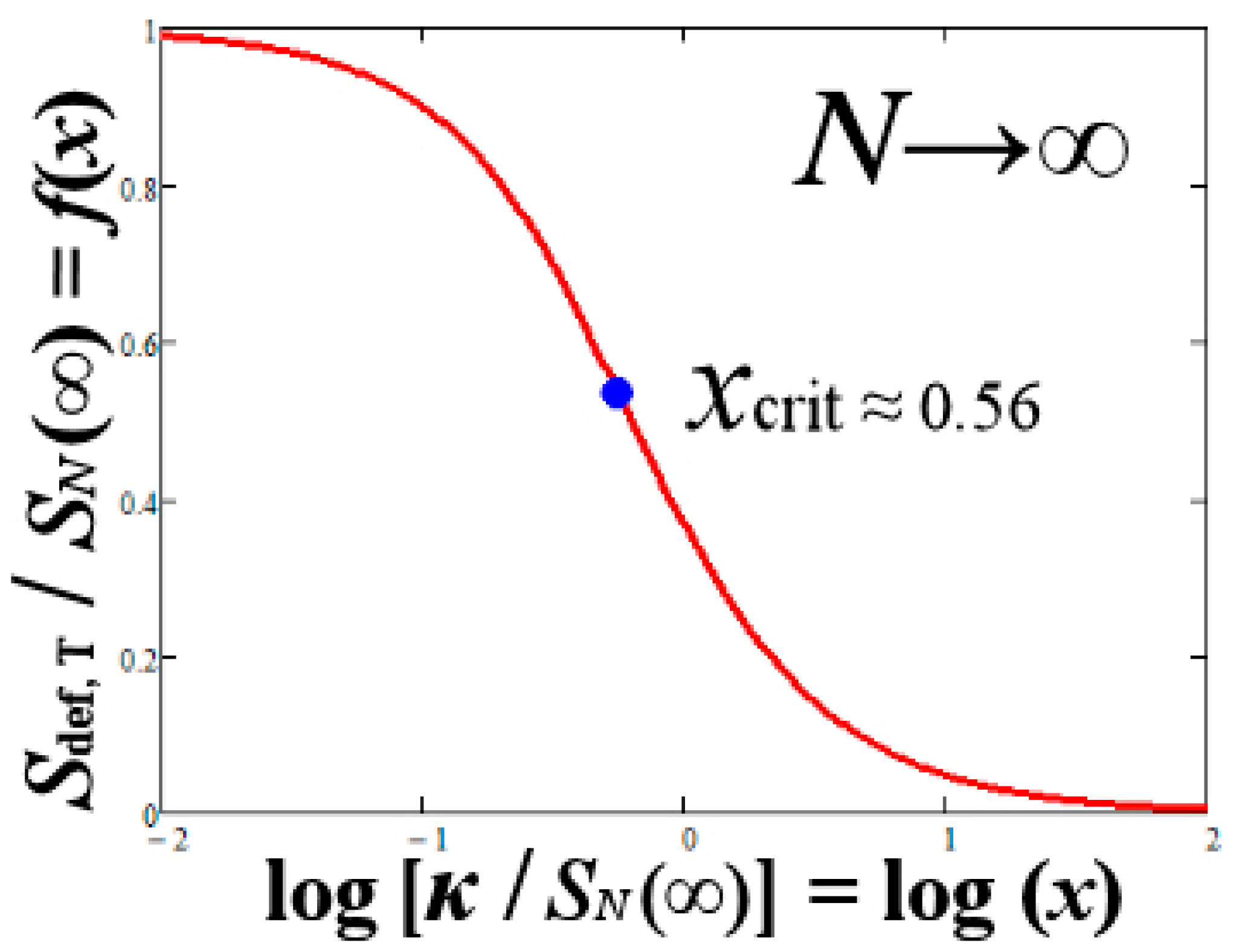
The total entropy defect of the system is used to find the relationship among the involved thermodynamic parameters, an optimal relationship between kappa and temperature is deduced, and the correlation coefficient is shown to be inversely proportional to the temperature logarithm.

Having brought the analogue of the classical mass defect to the concept of entropy and thermodynamics, it is then straightforward to apply the developed formalism and theoretical findings on the entropic defect to systems of charged particles in magnetic fields such as in space plasmas, where Debye shielding and magnetic fields can induce correlations among particles [33]. It is interesting that there may be examples that could be experimentally testable, which could include colloids and dusty plasmas with confinement [79,80,81].

Finally, in

Table 1. Table of the basic derived equations and formulae and their explanations.

Equations and Formulae	Explanation
$S_{\mathrm{A}+\mathrm{B}}=S_{\mathrm{A}}+S_{\mathrm{B}}-S_{\mathrm{def}}(S_{\mathrm{A}},S_{\mathrm{B}})$	Non-additive partitioning rule
$S_{\mathrm{def}}(S_{\mathrm{A}},S_{\mathrm{B}})=\frac{1}{\kappa }\cdot S_{\mathrm{A}}\cdot S_{\mathrm{B}}$	Entropy defect; this is proportional to the combining entropies $S_{\mathrm{A}}$ and $S_{\mathrm{B}}$; the proportionality constant defines kappa
$S_{\mathrm{ind}}{}_N$ or $S_N(\kappa \to \infty )$	Entropy of a system with no correlations among its constituents
$S_N$ or $S_N(\kappa )$	Entropy of a system with correlations among its constituents
${\exp }_{\kappa }(S_N)={\exp }_{(N\cdot \kappa )}(S_{\mathrm{ind}}{}_N)$ or $\begin{array}{c}{S}_N(\kappa )=\kappa \cdot \left\{1-{\exp }_N\left[-\frac{1}{\kappa }{S}_N(\infty )\right]\right\}\\ =\kappa \cdot \left\{1-{\left[1-\frac{1}{N\kappa }\cdot S_N(\infty )\right]}^N\right\}\end{array}$	Connection between the nonextensive entropy (actual entropy of a system with correlations) and the extensive entropy (entropy of the system if there were no correlations)
$S_N={\ln }_{\kappa }[\exp (S_{\mathrm{ind}}{}_N)]\iff S_{\mathrm{ind}}{}_N=\ln [{\exp }_{\kappa }(S_N)]$ or $S_N(\kappa )=\kappa \cdot \left\{1-\exp \left[-\frac{1}{\kappa }{S}_N(\infty )\right]\right\}$	Connection between the entropies for a large number of constituents, N >> 1
$S_{\mathrm{def},\mathrm{T}}\equiv S_N(\infty )-S_N(\kappa )$	Total entropy defect combined from all the constituents
$\frac{S_{\mathrm{def},\mathrm{T}}}{S_N(\infty )}=f(\frac{\kappa }{S_N(\infty )})$, $f(x)\equiv 1+x\cdot [{(1-\frac{1}{N\cdot x})}^N-1]$	Total entropy defect and its dependence on kappa
$S_{\mathrm{ind}}{}_N=\frac{1}{2}D\cdot N\cdot \ln (T/T_0)$	Extensive entropy in terms of temperature
$S_N=\kappa \cdot \left\{1-{\left[1-\frac{1}{\kappa }\cdot \frac{1}{2}D\cdot \ln (T/T_0)\right]}^N\right\}$ or $S_N=\kappa \cdot \left[1-{(T/T_0)}^{-\frac{1}{\kappa }\cdot \frac{1}{2}D\cdot N}\right]$, for N >> 1	Nonextensive entropy in terms of temperature
$k_{\mathrm{B}}{T}_0=C\cdot {\hslash }_{\mathrm{c}}^2{(m_{\mathrm{e}}{m}_{\mathrm{i}})}^{-\frac{1}{2}}\cdot {\mathsf{\lambda }}_{\mathrm{c}}^{-2}\cdot g_{\kappa ,N}$, where C = (9π/2)1/3/e ≈ 0.89, and $g_{\kappa ,N}={\left[\frac{\mathsf{\Gamma }({\kappa }_0)}{\sqrt{\frac{2\pi }{{\kappa }_0}}{\left(\frac{{\kappa }_0}{e}\right)}^{{\kappa }_0}}\cdot \frac{\sqrt{\frac{2\pi }{\kappa }}{\left(\frac{\kappa }{e}\right)}^{\kappa }}{\mathsf{\Gamma }(\kappa )}\cdot \sqrt{\frac{\kappa }{{\kappa }_0}}\right]}^{-\frac{2}{3}\cdot \frac{1}{N}}~1$, with ${\kappa }_0=\kappa -\frac{1}{2}D\cdot N$	Minimum temperature, T > T0, for the entropy to be positive; kB: Boltzmann constant, mi and me: ion and electron masses; λc: smallest correlation length, that is, the interparticle distance for collisional particle systems (absence of correlations), or by the Debye length for collisionless particle systems (presence of local correlations); the phase-space parcel ${\hslash }_{\mathrm{c}}^{}$ is given by the Planck’s constant, but it represents a larger constant in space plasmas.
$\frac{1}{T}\equiv {\left(\frac{\partial S_{\mathrm{ind}}}{\partial U}\right)}_{V,N}$ and $\frac{1}{T}\equiv \frac{\frac{1}{2}D}{\langle \epsilon \rangle }$	Thermodynamic and kinetic definitions of the (inverse) temperature
$\frac{1}{\kappa }\equiv \frac{1}{S}\cdot {\left(\frac{\partial S_{\mathrm{def}}}{\partial S_{\mathrm{ind}}}\right)}_{V,N}$ and $\frac{1}{\kappa }\equiv \frac{\rho }{\frac{1}{2}D}$	Thermodynamic and kinetic definitions of the (inverse) kappa
$\frac{1}{\kappa T}\equiv \frac{\rho }{\langle \epsilon \rangle }$, $\frac{1}{\kappa T}\equiv \frac{1}{S}\cdot {\left(\frac{\partial S_{\mathrm{def}}}{\partial U}\right)}_{V,N}$	Thermodynamic and kinetic definitions of the (inverse) product of kappa and temperature
$\langle \epsilon \rangle ~{\left(\frac{\partial U}{\partial S_{\mathrm{ind}}}\right)}_{V,N}$, $\rho ~\frac{1}{S}\cdot {\left(\frac{\partial S_{\mathrm{def}}}{\partial S_{\mathrm{ind}}}\right)}_{V,N}$	Kinetic definitions expressed in terms of thermodynamic definitions
$\kappa ~0.56\cdot \frac{1}{2}D\cdot \ln (T/T_0)$ or $\rho ~1.8\cdot {\left[\ln (T/T_0)\right]}^{-1}$	The entropy maximization leads to a linear relationship between the kappa and temperature logarithm; the correlation coefficient is inversely proportional to the temperature (per T0) logarithm
${\exp }_{\kappa }(x)\equiv {(1-\frac{1}{\kappa }x)}^{-\kappa }$, ${\ln }_{\kappa }(x)\equiv \kappa (1-x^{-\frac{1}{\kappa }})$ with ${\exp }_{\kappa }[{\ln }_{\kappa }(x)]={\ln }_{\kappa }[{\exp }_{\kappa }(x)]=x$	Definitions of the q-deformed exponential and logaritm (inverse) functions

we provide the basic equations and formulae derived in this paper.

References

1. Abe, S. General pseudoadditivity of composable entropy prescribed by the existence of equilibrium. Phys. Rev. E 2001, 63, 061105. [Google Scholar] [CrossRef] [Green Version]
2. Martínez, S.; Pennini, F.; Plastino, A. Thermodynamics’ zeroth law in a nonextensive scenario. Phys. A 2001, 295, 416–424. [Google Scholar] [CrossRef] [Green Version]
3. Livadiotis, G. Thermodynamic origin of kappa distributions. Europhys. Lett. 2018, 122, 50001. [Google Scholar] [CrossRef]
4. Toral, R. On the definition of physical temperature and pressure fornonextensive thermostatistics. Phys. A 2003, 317, 209–212. [Google Scholar] [CrossRef] [Green Version]
5. Livadiotis, G.; McComas, D.J. Beyond kappa distributions: Exploiting Tsallis statistical mechanics in space plasmas. J. Geophys. Res. 2009, 114, A11105. [Google Scholar] [CrossRef]
6. Livadiotis, G.; McComas, D.J. Exploring transitions of space plasmas out of equilibrium. Astrophys. J. 2010, 714, 971. [Google Scholar] [CrossRef]
7. Livadiotis, G. Approach on Tsallis statistical interpretation of hydrogen-atom by adopting the generalized radial distribution function. J. Math. Chem. 2009, 45, 930–939. [Google Scholar] [CrossRef]
8. Rajagopal, A.K.; Abe, S. Implications of form invariance to the structure of nonextensive entropies. Phys. Rev. Lett. 1999, 83, 1711. [Google Scholar] [CrossRef] [Green Version]
9. Wang, Q.A.; Nivanen, L.; Méhauté, A.L.; Pezeril, M. On the generalized entropy pseudoadditivity for complex systems. J. Phys. A 2002, 35, 7003–7007. [Google Scholar] [CrossRef] [Green Version]
10. Clausius, R.J.E. The Mechanical Theory of Heat; Taylor and Francis: London, UK, 1867. [Google Scholar]
11. Zemansky, M.W. Heat and Thermodynamics: An Intermediate Textbook, 5th ed.; McGraw-Hill: New York, NY, USA, 1968; p. 215. [Google Scholar]
12. Luzzi, R.; Vasconcellos, A.R.; Casas-Vázquez, J.; Jou, D. Characterization and measurement of a non-equilibrium temperature-like variable in irreversible thermodynamics. Phys. A 1997, 234, 699–714. [Google Scholar] [CrossRef]
13. Abe, S. Macroscopic thermodynamics based on composable nonextensive entropies. Phys. A 2002, 305, 62–68. [Google Scholar] [CrossRef]
14. Landsberg, P.T.; Vedral, V. Distributions and channel capacities in generalized statistical mechanics. Phys. Lett. A 1998, 247, 211. [Google Scholar] [CrossRef]
15. Wada, T.; Saito, T. The additivity of the pseudo-additive conditional entropy for a proper Tsallis’ entropic index. Phys. A 2002, 305, 186–189. [Google Scholar] [CrossRef] [Green Version]
16. Tsallis, C.; Gell-Mann, M.; Sato, Y. Asymptotically scale-invariant occupancy of phase space makes the entropy Sq extensive. Proc. Natl. Acad. Sci. USA 2005, 102, 15377–15382. [Google Scholar] [CrossRef] [Green Version]
17. Sato, Y.; Tsallis, C. On the extensivity of the entropy Sq for N ≤ 3 specially correlated binary subsystems. Int. J. Bifurcat. Chaos 2006, 16, 1727–1738. [Google Scholar] [CrossRef]
18. Tsallis, C. Possible generalization of Boltzmann-Gibbs statistics. J. Stat. Phys. 1988, 52, 479. [Google Scholar] [CrossRef]
19. Tsallis, C.; Mendes, R.S.; Plastino, A.R. The role of constraints within generalized nonextensive statistics. Phys. A 1998, 261, 534–554. [Google Scholar] [CrossRef]
20. Gell-Mann, M.; Tsallis, C. Nonextensive Entropy: Interdisciplinary Applications; Oxford University Press: New York, NY, USA, 2004. [Google Scholar]
21. Livadiotis, G.; McComas, D.J. Understanding kappa distributions: A toolbox for space science and astrophysics. Space Sci. Rev. 2013, 75, 183–214. [Google Scholar] [CrossRef] [Green Version]
22. Livadiotis, G. Statistical background and properties of kappa distributions in space plasmas. J. Geophys. Res. 2015, 120, 1607–1619. [Google Scholar] [CrossRef]
23. Livadiotis, G. Kappa Distribution: Theory & Applications in Plasmas, 1st ed.; Elsevier: Amsterdam, The Netherlands, 2017. [Google Scholar]
24. Livadiotis, G. Kappa Distributions: Statistical Physics and Thermodynamics of Space and Astrophysical Plasmas. Universe 2018, 4, 144. [Google Scholar] [CrossRef] [Green Version]
25. Binsack, J.H. Plasma Studies with the IMP-2 Satellite. Ph.D. Thesis, Massachusetts Institute of Technology, Cambridge, MA, USA, 1966. [Google Scholar]
26. Olbert, S. Summary of experimental results from M.I.T. detector on IMP-1. In Physics of the Magnetosphere; Carovillano, R.L., McClay, J.F., Radoski, H.R., Eds.; Springer: New York, NY, USA, 1968; p. 641. [Google Scholar]
27. Vasyliũnas, V.M. A survey of low-energy electrons in the evening sector of the magnetosphere with OGO 1 and OGO 3. J. Geophys. Res. 1968, 73, 2839–2884. [Google Scholar] [CrossRef]
28. Treumann, R.A. Theory of superdiffusion for the magnetopause. Geophys. Res. Lett. 1997, 24, 1727–1730. [Google Scholar] [CrossRef]
29. Milovanov, A.V.; Zelenyi, L.M. Functional background of the Tsallis entropy: “coarse-grained” systems and “kappa” distribution functions. Nonlinear Process. Geophys. 2000, 7, 211–221. [Google Scholar] [CrossRef] [Green Version]
30. Leubner, M.P. A nonextensive entropy approach to kappa distributions. Astrophys. Space Sci. 2002, 282, 573–579. [Google Scholar] [CrossRef]
31. Tsallis, C. Introduction to Nonextensive Statistical Mechanics; Springer: New York, NY, USA, 2009. [Google Scholar]
32. Livadiotis, G.; McComas, D.J. Measure of the departure of the q-metastable stationary states from equilibrium. Phys. Scr. 2010, 82, 035003. [Google Scholar] [CrossRef]
33. Livadiotis, G.; Desai, M.I.; Wilson, L.B., III. Generation of kappa distributions in solar wind at 1 AU. Astrophys. J. 2018, 853, 142. [Google Scholar] [CrossRef]
34. Shizgal, B.D. Kappa and other nonequilibrium distributions from the Fokker-Planck equation and the relationship to Tsallis entropy. Phys. Rev. E 2018, 97, 052144. [Google Scholar] [CrossRef] [PubMed]
35. Livadiotis, G. Using kappa distributions to identify the potential energy. J. Geophys. Res. 2018, 123, 1050–1060. [Google Scholar] [CrossRef]
36. Yoon, P. Classical Kinetic Theory of Weakly Turbulent Nonlinear Plasma Processes; Cambridge University Press: Cambridge, MA, USA, 2019. [Google Scholar]
37. Livadiotis, G. On the simplification of statistical mechanics for space plasmas. Entropy 2017, 19, 285. [Google Scholar] [CrossRef] [Green Version]
38. Livadiotis, G. Derivation of the entropic formula for the statistical mechanics of space plasmas. Nonlinear Process. Geophys. 2018, 25, 77–88. [Google Scholar] [CrossRef] [Green Version]
39. Suyari, H. Nonextensive entropies derived from form invariance of pseudoadditivity. Phys. Rev. E 2002, 65, 066118. [Google Scholar] [CrossRef] [Green Version]
40. Ilic, V.M.; Stankovic, M.S. Comments on “Nonextensive entropies derived from Form Invariance of Pseudoadditivity”. arXiv 2012, arXiv:1210.7473. [Google Scholar]
41. Lavenda, B.H. Thermodynamics of Irreversible Processes; Macmillan: London, UK, 1978. [Google Scholar]
42. Schroeder, D. An Introduction to Thermal Physics; Addison Wesley Longman: Boston, MA, USA, 2000; pp. 20–21. [Google Scholar]
43. Livadiotis, G.; McComas, D.J. Invariant kappa distribution in space plasmas out of equilibrium. Astrophys. J. 2011, 741, 88. [Google Scholar] [CrossRef] [Green Version]
44. Elaydi, S. An Introduction to Difference Equations; Springer: New York, NY, USA, 2005. [Google Scholar]
45. Livadiotis, G. Numerical approximation of the percentage of order for one-dimensional maps. Adv. Complex Sys. 2005, 8, 15–32. [Google Scholar] [CrossRef]
46. Kwessi, E.; Elaydi, S.; Livadiotis, G.; Dennis, B. Nearly exact discretization of single species population models. Nat. Res. Mod. 2018, 31, e12167. [Google Scholar] [CrossRef]
47. Nivanen, L.; Le Mehaute, A.; Wang, Q.A. Generalized algebra within a nonextensive statistics. Rep. Math. Phys. 2003, 52, 437–444. [Google Scholar] [CrossRef] [Green Version]
48. Borges, E.P. A possible deformed algebra and calculus inspired in nonextensive thermostatistics. Phys. A 2004, 340, 95–101. [Google Scholar] [CrossRef] [Green Version]
49. Suyari, H. Mathematical structures derived from the q-multinomial coefficient in Tsallis statistics. Phys. A 2006, 368, 63–82. [Google Scholar] [CrossRef]
50. Suyari, H.; Saito, T. Scaling property and the generalized entropy uniquely determined by a fundamental nonlinear differential equation. arXiv 2006, arXiv:cond-mat/0608007. [Google Scholar]
51. Abe, S. Correlation induced by Tsallis’ nonextensivity. Phys. A 1999, 269, 403–409. [Google Scholar] [CrossRef]
52. Asgarani, S.; Mirza, B. Quasi-additivity of Tsallis entropies and correlated subsystems. Phys. A 2007, 379, 513–522. [Google Scholar] [CrossRef] [Green Version]
53. Livadiotis, G. Kappa and q indices: Dependence on the degrees of freedom. Entropy 2015, 17, 2062. [Google Scholar] [CrossRef] [Green Version]
54. Livadiotis, G.; Nicolaou, G.; Allegrini, F. Anisotropic kappa distributions. I. Formulation based on particle correlations. Astrophys. J. Suppl. Ser. 2021, 253, 16. [Google Scholar] [CrossRef]
55. Livadiotis, G.; McComas, D.J. Evidence of large scale phase space quantization in plasmas. Entropy 2013, 15, 1118–1132. [Google Scholar] [CrossRef] [Green Version]
56. Livadiotis, G. Lagrangian temperature: Derivation and physical meaning for systems described by kappa distributions. Entropy 2014, 16, 4290–4308. [Google Scholar] [CrossRef] [Green Version]
57. Livadiotis, G.; McComas, D.J. Electrostatic shielding in plasmas and the physical meaning of the Debye length. J. Plasma Phys. 2014, 80, 341–378. [Google Scholar] [CrossRef] [Green Version]
58. Livadiotis, G. On the generalized formulation of Debye shielding in plasmas. Phys. Plasmas 2019, 26, 050701. [Google Scholar] [CrossRef] [Green Version]
59. Livadiotis, G.; McComas, D.J. Large-scale quantization from local correlations in space plasmas. J. Geophys. Res. 2014, 119, 3247–3258. [Google Scholar] [CrossRef]
60. Scholkmann, F. A prediction of an additional planet of the extrasolar planetary system Kepler-62 based on the planetary distances’ long-range order. Prog. Phys. 2013, 4, 85–89. [Google Scholar]
61. Livadiotis, G.; Desai, M.I. Plasma-field coupling at small length scales in solar wind near 1 au. Astrophys. J. 2016, 829, 88. [Google Scholar] [CrossRef]
62. Livadiotis, G. Turbulent heating in Solar Wind Thermodynamics. Astrophys. J. 2019, 887, 117. [Google Scholar] [CrossRef]
63. Livadiotis, G.; Dayeh, M.A.; Zank, G. Estimation of turbulent heating of solar wind protons at 1 au. Astrophys. J. 2020, 905, 137. [Google Scholar] [CrossRef]
64. Sackur, O. Die Anwendung der kinetischen Theorie der Gase auf chemische Probleme (The application of the kinetic theory of gases to chemical problems). Ann. Phys. 1911, 36, 958–980. [Google Scholar] [CrossRef] [Green Version]
65. Tetrode, O. Die chemische Konstante der Gase und das elementare Wirkungsquantum (The chemical constant of gases and the elementary quantum of action). Ann. Phys. 1912, 38, 434–442. [Google Scholar] [CrossRef] [Green Version]
66. Baeten, M.; Naudts, J. On the Thermodynamics of Classical Micro-Canonical Systems. Entropy 2011, 13, 1186–1199. [Google Scholar] [CrossRef] [Green Version]
67. Collier, M.R.; Hamilton, D.C. The relationship between kappa and temperature in the energetic ion spectra at Jupiter. Geophys. Res. Lett. 1995, 22, 303–306. [Google Scholar] [CrossRef]
68. Livadiotis, G.; McComas, D.J.; Dayeh, M.A.; Funsten, H.O.; Schwadron, N.A. First sky map of the inner heliosheath temperature using IBEX spectra. Astrophys. J. 2011, 734, 1. [Google Scholar] [CrossRef] [Green Version]
69. Livadiotis, G.; McComas, D.J. Non-equilibrium thermodynamic processes: Space plasmas and the inner heliosheath. Astrophys. J. 2012, 749, 11. [Google Scholar] [CrossRef]
70. Ogasawara, K.; Angelopoulos, V.; Dayeh, M.A.; Fuselier, S.A.; Livadiotis, G.; McComas, D.J.; McFadden, J.P. Characterizing the dayside magnetosheath using ENAs: IBEX and THEMIS observations. J. Geophys. Res. 2013, 118, 3126–3137. [Google Scholar] [CrossRef]
71. Broiles, T.W.; Livadiotis, G.; Burch, J.L.; Chae, K.; Clark, G.; Cravens, T.E.; Davidson, R.; Eriksson, A.; Frahm, R.A.; Fuselier, S.A.; et al. Characterizing cometary electrons with kappa distributions. J. Geophys. Res. 2016, 121, 7407–7422. [Google Scholar] [CrossRef] [Green Version]
72. Dialynas, K.; Roussos, E.; Regoli, L.; Paranicas, C.P.; Krimigis, S.M.; Kane, M.; Mitchell, D.G.; Hamilton, D.C.; Krupp, N.; Carbary, J.F. Energetic ion moments and polytropic index in Saturn’s magnetosphere using Cassini/MIMI measurements: A simple model based on κ-distribution functions. J. Geophys. Res. 2018, 123, 8066–8086. [Google Scholar] [CrossRef]
73. Nicolaou, G.; Livadiotis, G. Long-term correlations of polytropic indices with kappa distributions in solar wind plasma near 1 au. Astrophys. J. 2019, 884, 52. [Google Scholar] [CrossRef]
74. McComas, D.J.; Allegrini, F.; Bochsler, P.; Bzowski, M.; Collier, M.; Fahr, H.; Fichtner, H.; Frisch, P.; Funsten, H.O.; Fuselier, S.A.; et al. IBEX—Interstellar Boundary Explorer. Space Sci. Rev. 2009, 146, 11–33. [Google Scholar] [CrossRef] [Green Version]
75. McComas, D.J.; Allegrini, F.; Bochsler, P.; Bzowski, M.; Christian, E.R.; Crew, G.B.; DeMajistre, R.; Fahr, H.; Fichtner, H.; Frisch, P.C.; et al. Global Observations of the Interstellar Interaction from the Interstellar Boundary Explorer (IBEX). Science 2009, 326, 959. [Google Scholar] [CrossRef] [PubMed]
76. Funsten, H.O.; Allegrini, F.; Crew, G.B.; DeMajistre, R.; Frisch, P.C.; Fuselier, S.A.; Gruntman, M.; Janzen, P.; McComas, D.J.; Möbius, E.; et al. Structures and Spectral Variations of the Outer Heliosphere in IBEX Energetic Neutral Atom Maps. Science 2009, 326, 964. [Google Scholar] [CrossRef]
77. Livadiotis, G.; McComas, D.J.; Randol, B.M.; Funsten, H.O.; Möbius, E.S.; Schwadron, N.A.; Dayeh, M.A.; Zank, G.P.; Frisch, P.C. Pick-up ion distributions and their influence on energetic neutral atom spectral curvature. Astrophys. J. 2012, 751, 64. [Google Scholar] [CrossRef] [Green Version]
78. Swaczyna, P.; McComas, D.J.; Schwadron, N.A. Non-equilibrium distributions of interstellar neutrals and the temperature of the local interstellar medium. Astrophys. J. 2019, 871, 274. [Google Scholar] [CrossRef]
79. Ying-Ju, L.; Lin, I. Defects and particle motions in the nonuniform melting of a two-dimensional Coulomb cluster. Phys. Rev. E 2001, 64, 015601. [Google Scholar]
80. Drocco, J.A.; Reichhardt, C.J.; Reichhardt, C.; Jankó, B. Structure and melting of two-species charged clusters in a parabolic trap. Phys. Rev. E 2003, 68, 060401. [Google Scholar] [CrossRef] [PubMed] [Green Version]
81. Yang, W.; Kong, M.; Milošević, M.V.; Zeng, Z.; Peeters, F.M. Two-dimensional binary clusters in a hard-wall trap: Structural and spectral properties. Phys. Rev. E 2007, 76, 041404. [Google Scholar] [CrossRef] [PubMed]
82. Beck, C.; Schlögl, F. Thermodynamics of Chaotic Systems; Cambridge University Press: Cambridge, UK, 1993. [Google Scholar]
Figure 1. (a) The entropy of a system with no correlations among its constituents is additive. (b) However, the formation of a system with interactions inducing correlations (such as long-range interactions) requires its entropy to follow a nonadditive rule in terms of the entropies of the subsystems (composability). The difference among the total entropy and the sum of the subsystem entropies equals a missing amount of entropy, the “entropy defect” (Equation (5)), which is a decrease of entropy due to the order generated by the presence of correlations. Later in this paper, we develop the formulae connecting correlations (kinetic definition of the kappa index) with the entropy defect (thermodynamic definition of the kappa index).
Entropy 23 01683 g001
Figure 2. Diagram of entropy differences (equivalent to energy level per temperature) with respect to the time evolution during the composition of a system, when (a) it is composed by two subsystems A and B, as shown in Equations (5) and (6), and (b) an independent elementary subsystem is added to it, as shown in Equations (7) and (8). The entropy of the system with correlations is lower than the entropy of the system if there were no correlations, because the correlations add order to the system; at the composition of the system, its entropy differs from the sum of the subsystem entropies by the entropy defect.
Entropy 23 01683 g002
Figure 3. The relationship between the entropy of a system, SN, composed by N originally independent subsystems, and the respective extensive entropy, SindN, that is, the sum of the subsystem entropies, dSindN = SindN/N. The statistical weight W is independent of the kappa index, for a fixed value of the extensive entropy of the system SindN (i.e., for dSindN 1/N) and at the limit of N >> 1. The missing entropy, that is, the difference between the extensive SindN and the nonextensive SN entropic values, is caused by the presence of correlations and is interpreted and expressed as an entropy defect. As shown in Figure 2, the entropy of the system with correlations, SN, is lower than the entropy of the system if there were no correlations, SindN, because the correlations add order to the system; the missing entropy gives the entropy defect.
Entropy 23 01683 g003
Figure 4. Plot of the function f with respect to the logarithm of x κ / S N ( ) , as shown in Equation (59). This function gives the total entropic defect of a composed system, normalized to the total entropy, for a large number N. (The critical value corresponds to the point of inflection, which is where the defect decreases at a slower rate with increasing of log (x)).
Entropy 23 01683 g004