Figure 1.
Physical structure of UP-EHD flow model.
Figure 1.
Physical structure of UP-EHD flow model.
Figure 2.
Work flow chartof proposed methodology. Initially, population in SCA is set for generation of solutions, fitness of generated solution is evaluated by SCA. The fittest solution is provided as an initial point to SQP and SQP provides the best solution as weights of ANN.
Figure 2.
Work flow chartof proposed methodology. Initially, population in SCA is set for generation of solutions, fitness of generated solution is evaluated by SCA. The fittest solution is provided as an initial point to SQP and SQP provides the best solution as weights of ANN.
Figure 3.
The architecture of ANN model. With input points. It’s the simplest form of ANN. A unidirectional network with no cycle has three layers input, hidden, and output layers. In inputs,
is taken for an initial guess of unknown weights. For the hidden layer, sigmoid function is used as given in Equation (
12).
Figure 4.
Dynamic structure of UP-EHD based on variation of its parameters.
Figure 4.
Dynamic structure of UP-EHD based on variation of its parameters.
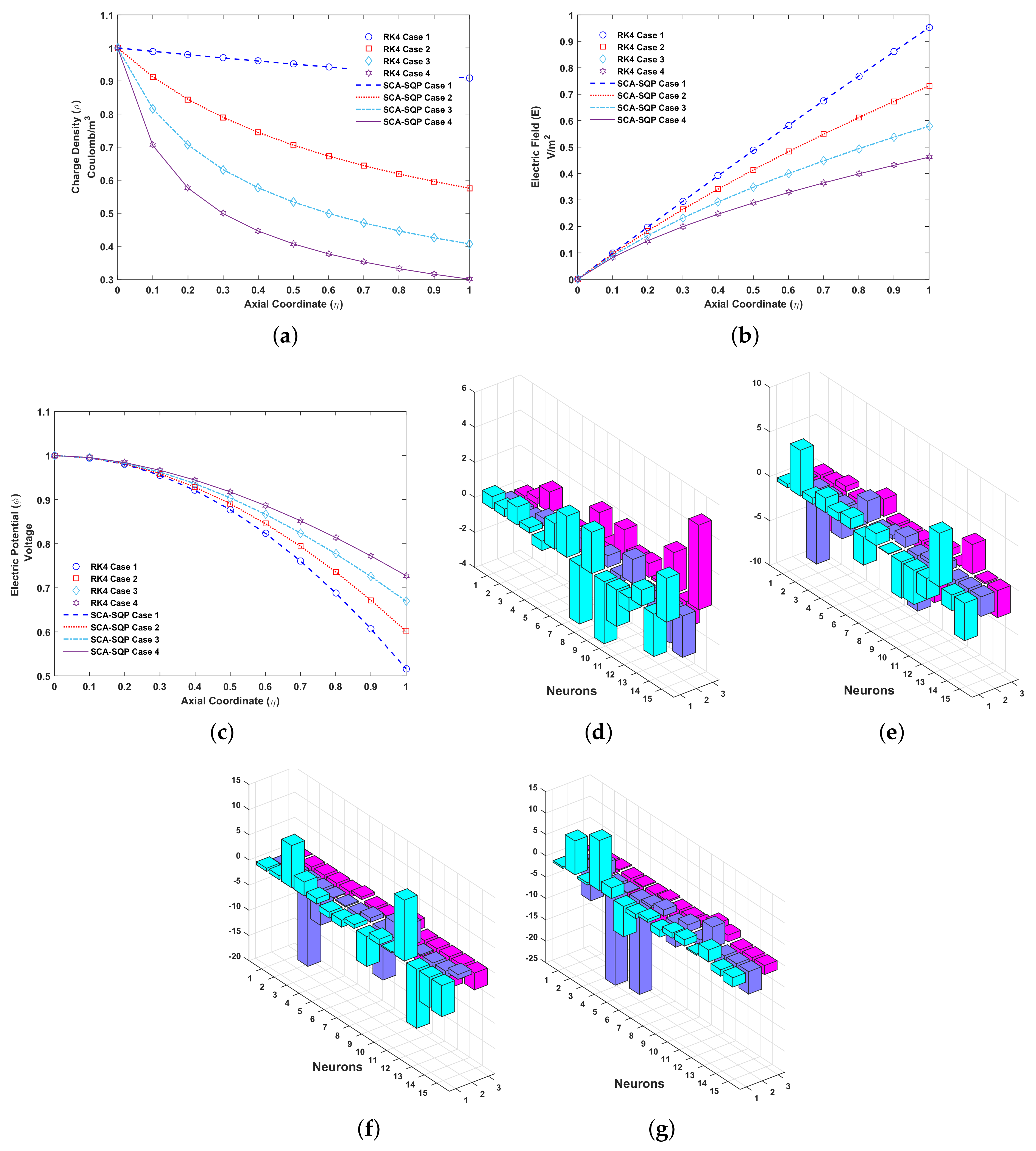
Figure 5.
Problem 1: (a). Charge density ()-Axial coordinate () graph for all cases, (b). Electric field (E)-Axial coordinate () graph for all cases, (c). Electric potential ()-Axial coordinate () graph for all cases, (d). Weights of case 1, (e). Weights of case 2, (f). Weights of case 3, (g). Weights of case 4.
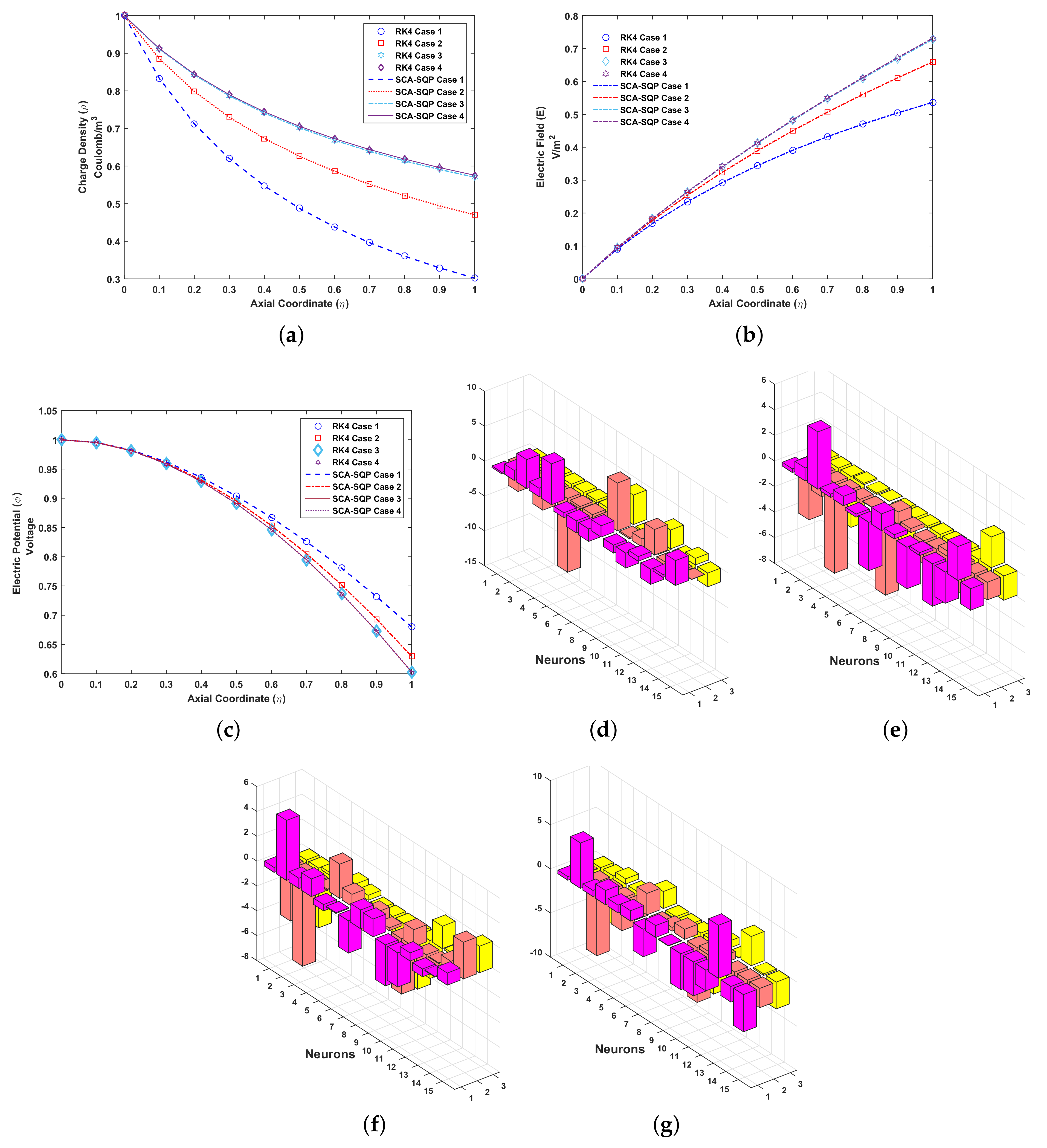
Figure 6.
Problem 2: (a). Charge density ()-Axial coordinate () graph for all cases, (b). Electric field (E)-Axial coordinate () graph for all cases, (c). Electric potential ()-Axial coordinate () graph for all cases, (d). Weights of case 1, (e). Weights of case 2, (f). Weights of case 3, (g). Weights of case 4.
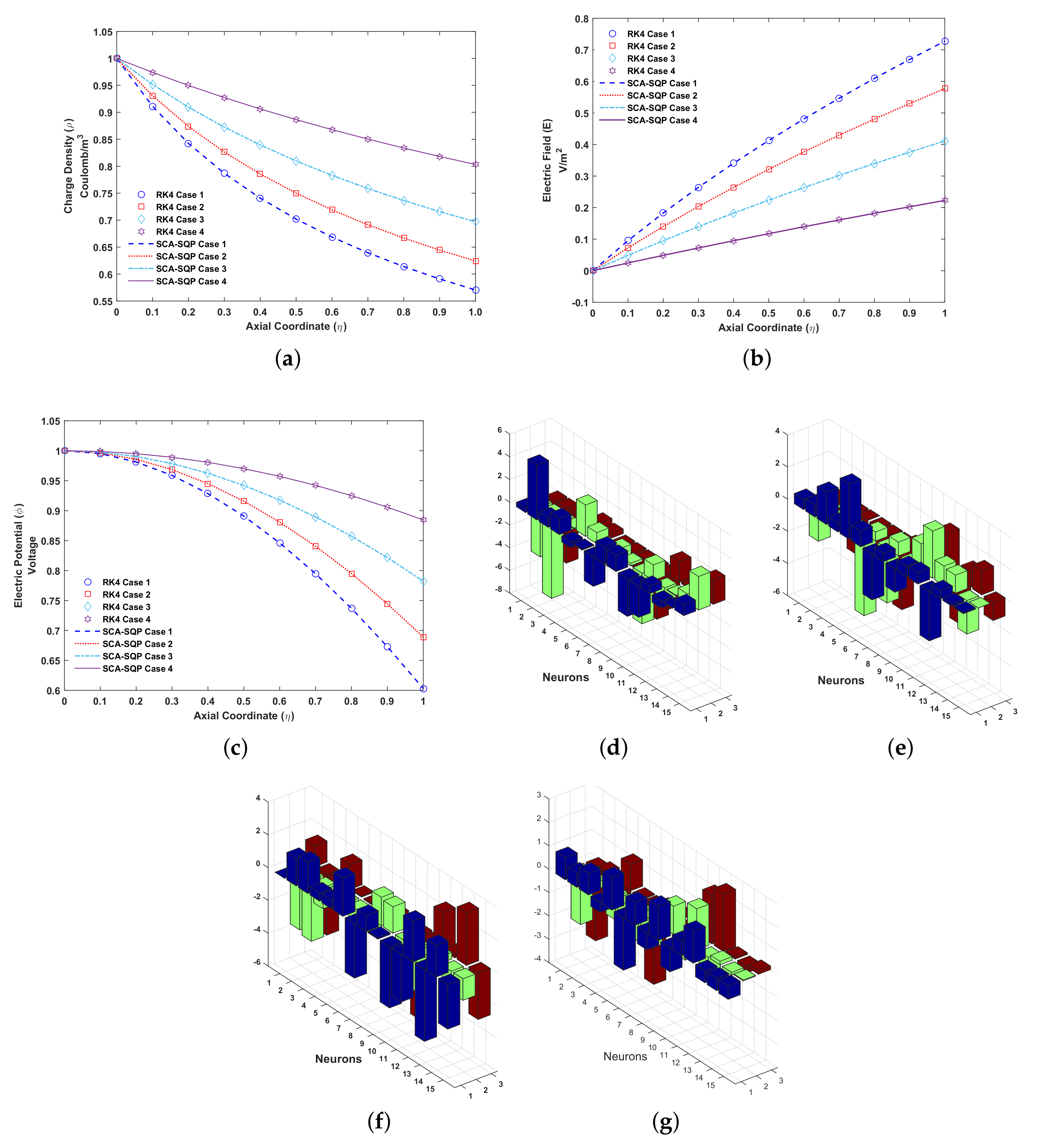
Figure 7.
Problem 3: (a). Charge density ()-Axial coordinate () graph for all cases, (b). Electric field (E)-Axial coordinate () graph for all cases, (c). Electric potential ()-Axial coordinate () graph for all cases, (d). Weights of case 1, (e). Weights of case 2, (f). Weights of case 3, (g). Weights of case 4.
Figure 8.
(a). Fitness of problem 1 all cases for , (b). Fitness of problem 1 all cases for E, (c). Fitness of problem 1 all cases for , (d). Fitness of problem 2 all cases for , (e). Fitness of problem 2 all cases for E, (f). Fitness of problem 2 all cases for , (g). Fitness of problem 3 all cases for , (h). Fitness of problem 3 all cases for E, (i). Fitness of problem 3 all cases for .
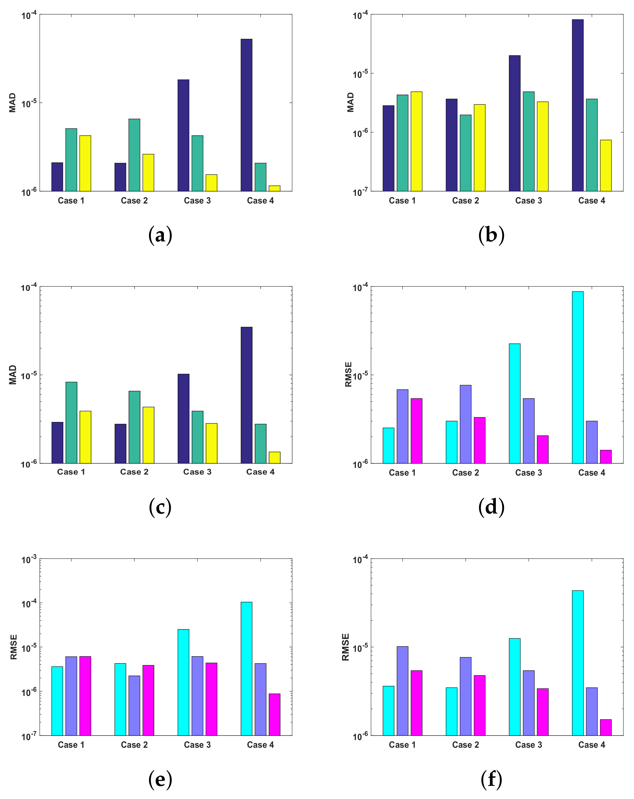
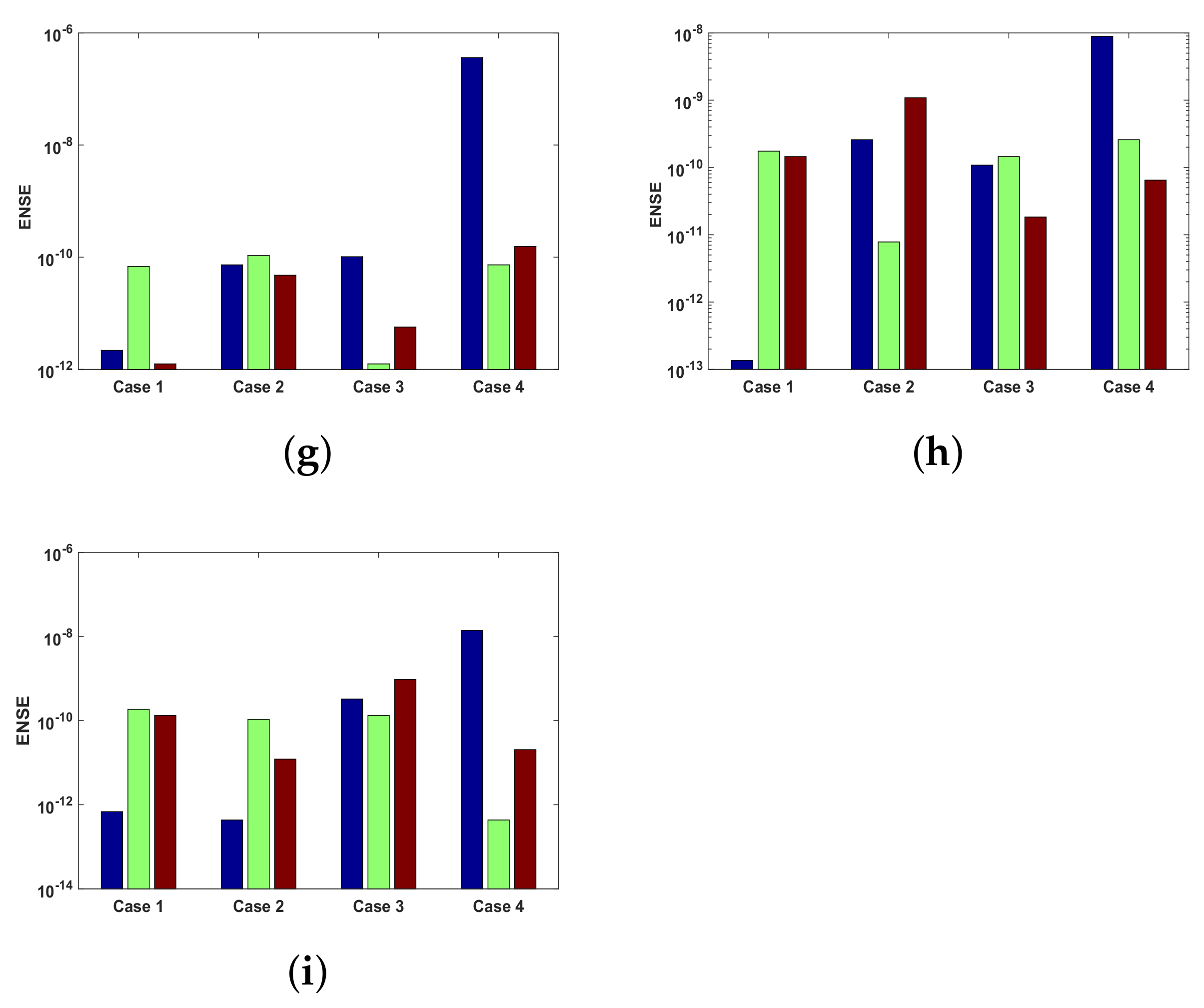
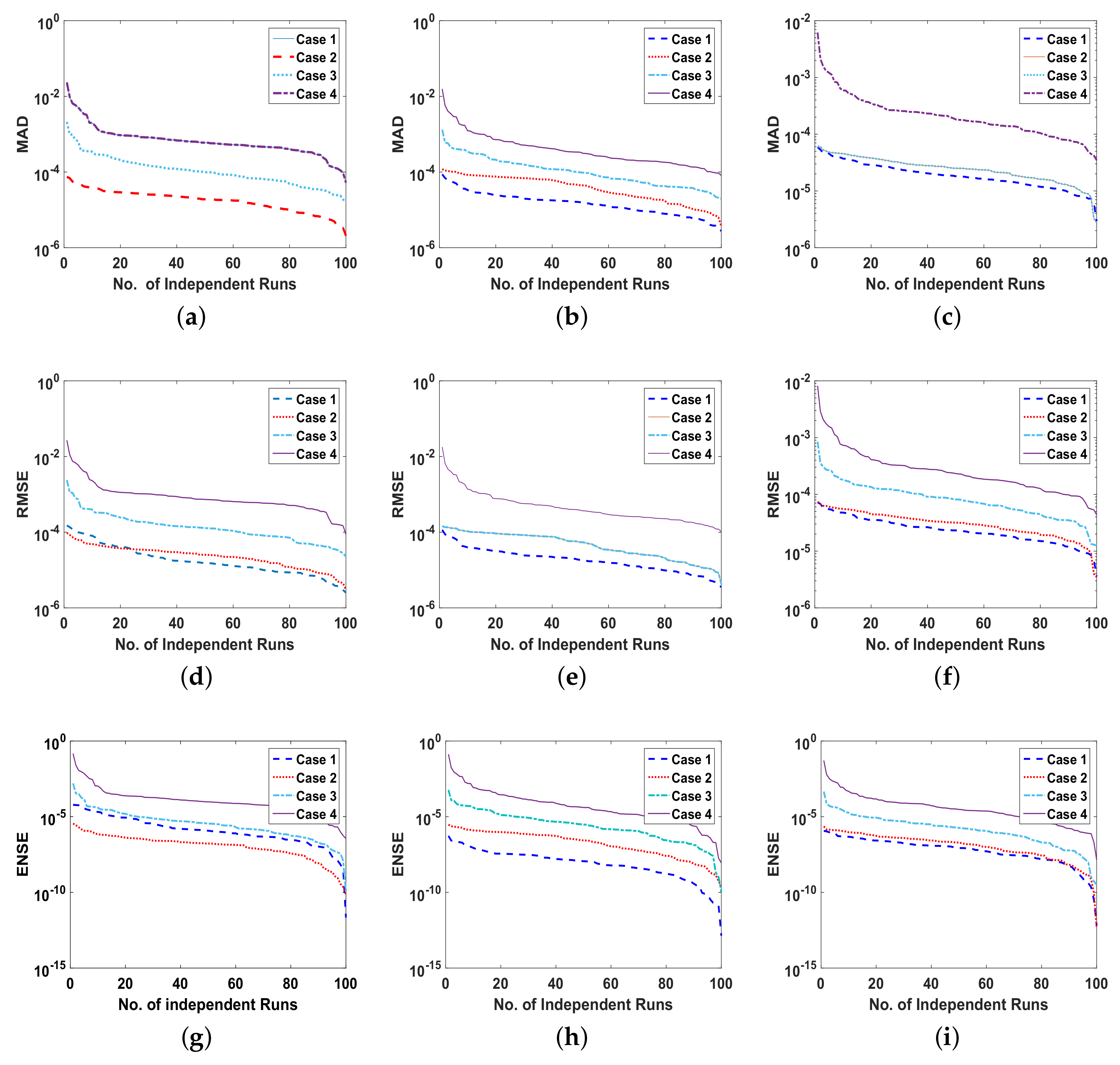
Figure 9.
(a). MAD of problem 1, all cases, (b). MAD of problem 2, all cases, (c). MAD of problem 3, all cases, (d). RMSE of problem 1, all cases, (e). RMSE of problem 2, all cases, (f). RMSE of problem 3, all cases, (g). ENSE of problem 1, all cases, (h). ENSE of problem 2, all cases, (i). ENSE of problem 3, all cases.
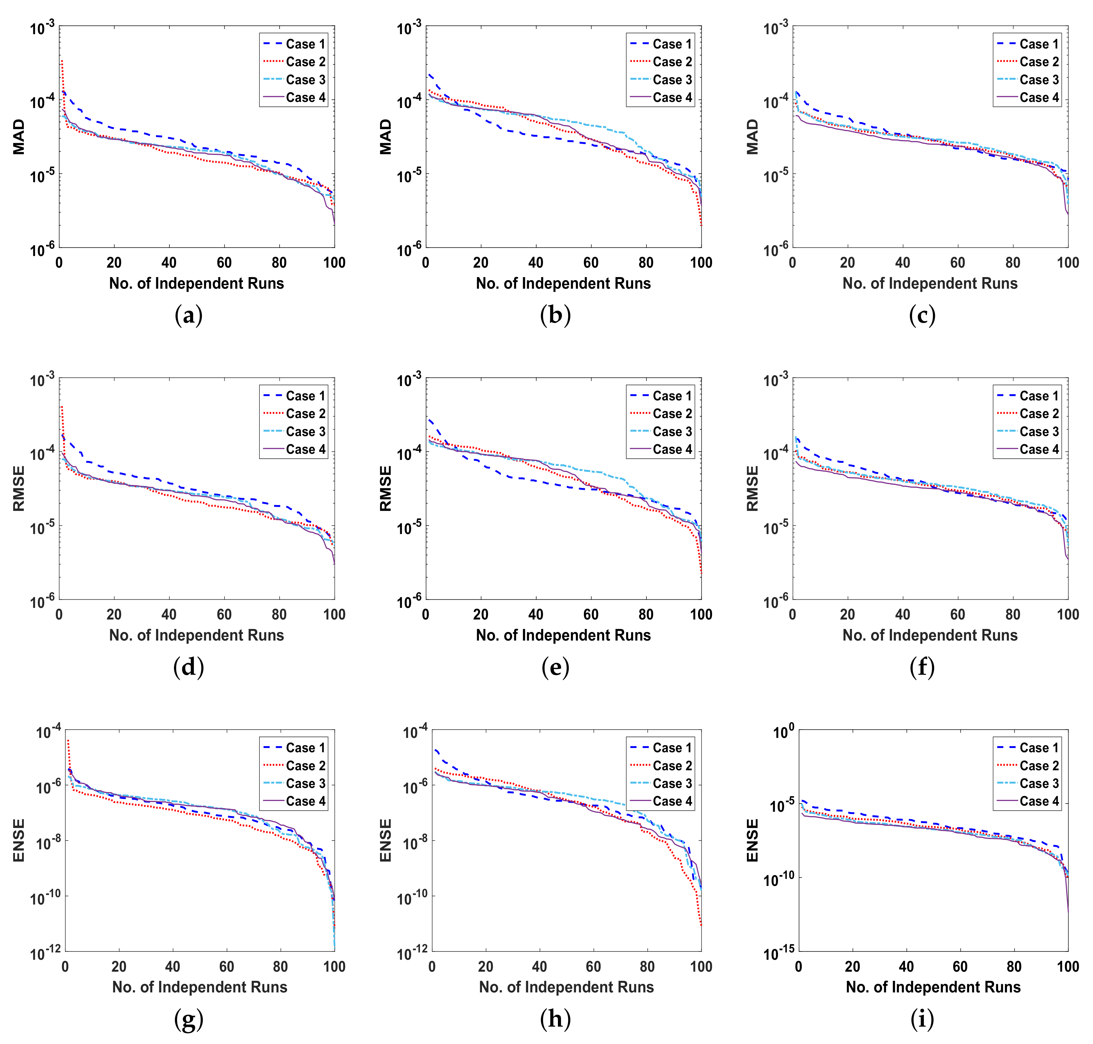
Figure 10.
(a). MAD of , for problem 1 all cases, (b). MAD of E, for problem 1 all cases, (c). MAD of , for problem 1 all cases, (d). RMSE of , for problem 1 all cases, (e). RMSE of E, for problem 1 all cases, (f). RMSE of , for problem 1 all cases, (g). ENSE of , for problem 1 all cases, (h). ENSE of E, for problem 1 all cases, (i). ENSE of , for problem 1 all cases.
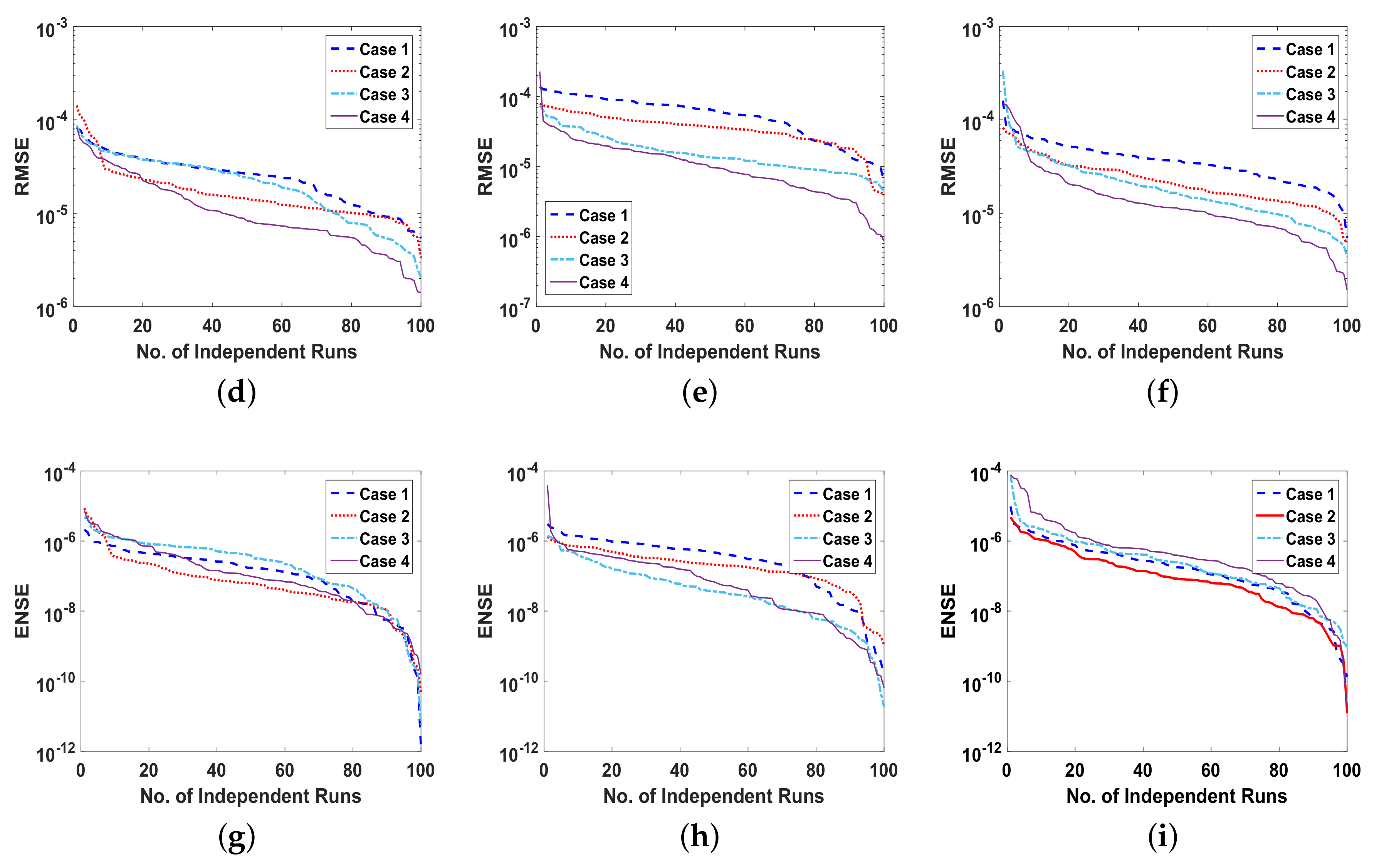
Figure 11.
(a). MAD of , for problem 2 all cases, (b). MAD of E, for problem 2 all cases, (c). MAD of , for problem 2all cases, (d). RMSE of , for problem 2 all cases, (e). RMSE of E, for problem 2 all cases, (f). RMSE of , for problem 2 all cases, (g). ENSE of , for problem 2 all cases, (h). ENSE of E, for problem 2 all cases, (i). ENSE of , for problem 2 all cases.
Figure 12.
(a). MAD of , for problem 3 all cases, (b). MAD of E, for problem 3 all cases, (c). MAD of , for problem 3, all cases, (d). RMSE of , for problem 3 all cases, (e). RMSE of E, for problem 3 all cases, (f). RMSE of , for problem 3 all cases, (g). ENSE of , for problem 3 all cases, (h). ENSE of E, for problem 3 all cases, (i). ENSE of , for problem 3 all cases.
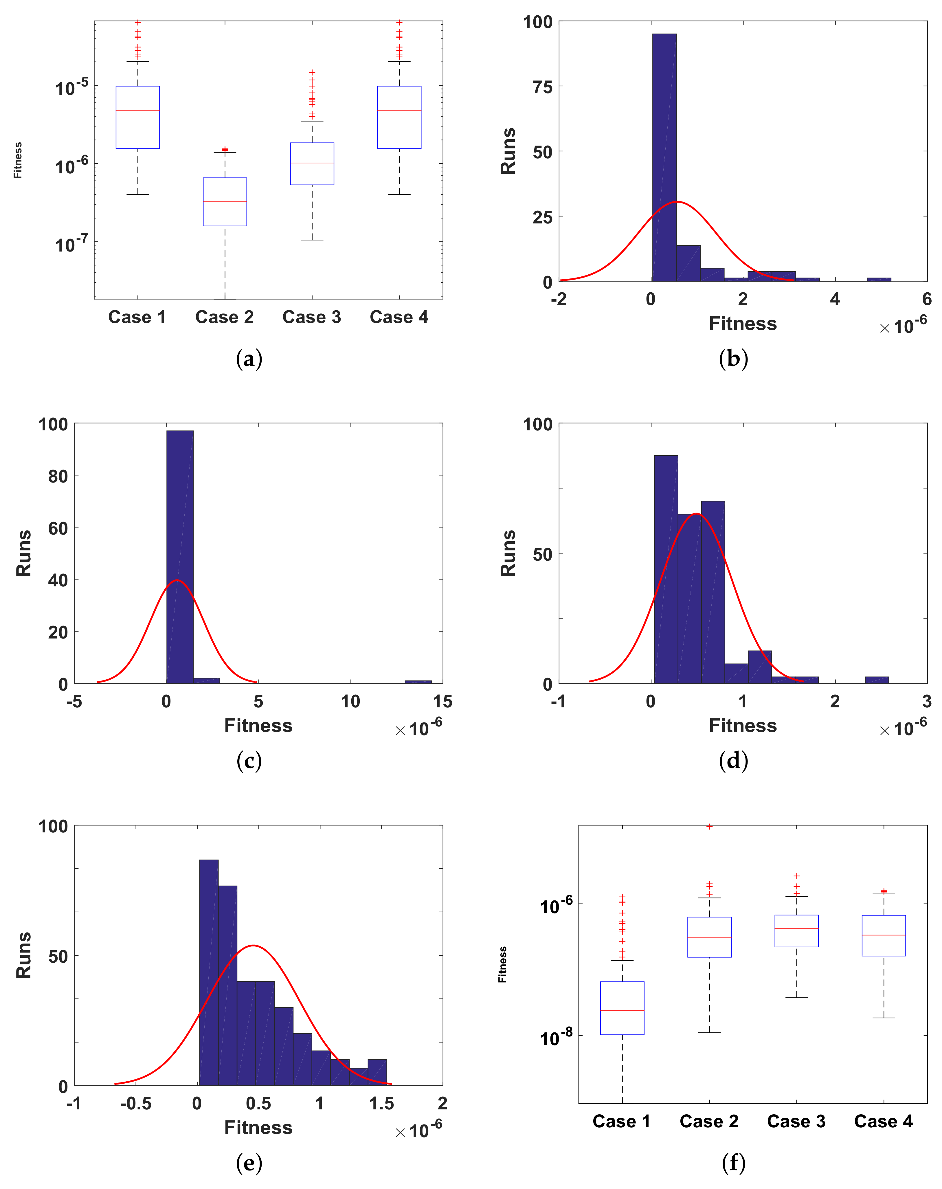
Figure 13.
(a). Fitness of , problem 1 all cases, (b). Fitness of E, problem 2 case 1, (c). Fitness of E, problem 2 case 2, (d). Fitness of E, problem 2 case 3, (e). Fitness of E, problem 2 case 4, (f). Fitness of , problem 3 all cases.
Figure 13.
(a). Fitness of , problem 1 all cases, (b). Fitness of E, problem 2 case 1, (c). Fitness of E, problem 2 case 2, (d). Fitness of E, problem 2 case 3, (e). Fitness of E, problem 2 case 4, (f). Fitness of , problem 3 all cases.
Table 1.
Absolute errors of problem 1 for different inputs in terms of minimum, maximum, mean and standard deviation.
Table 1.
Absolute errors of problem 1 for different inputs in terms of minimum, maximum, mean and standard deviation.
| | Case | Mode | Absolute Errors for Inputs “” |
|---|
| = 0 | = 0.1 | = 0.2 | = 0.3 | = 0.4 | = 0.5 | = 0.6 | = 0.7 | = 0.8 | = 0.9 | = 1.0 |
|---|
| 1 | MIN | 5.30 × | 1.58 × | 1.41 × | 1.40 × | 1.54 × | 1.71 × | 1.36 × | 1.20 × | 1.28 × | 1.51 × | 3.57 × |
| MAX | 3.42 × | 8.17 × | 9.06 × | 9.05 × | 9.01 × | 1.11 × | 9.44 × | 7.08 × | 7.68 × | 8.73 × | 2.19 × |
| MEAN | 3.38 × | 1.80 × | 9.93 × | 1.29 × | 1.29 × | 8.91 × | 1.20 × | 1.08 × | 8.06 × | 1.46 × | 2.38 × |
| STD | 5.30 × | 1.58 × | 1.41 × | 1.40 × | 1.54 × | 1.71 × | 1.36 × | 1.20 × | 1.28 × | 1.51 × | 3.57 × |
| 2 | MIN | 4.95 × | 3.29 × | 4.82 × | 7.00 × | 9.74 × | 5.55 × | 6.61 × | 5.95 × | 7.25 × | 1.11 × | 1.51 × |
| MAX | 2.13 × | 5.76 × | 1.10 × | 2.21 × | 1.77 × | 1.33 × | 7.35 × | 1.55 × | 1.96 × | 1.08 × | 2.46 × |
| MEAN | 3.38 × | 1.31 × | 2.58 × | 3.95 × | 4.72 × | 2.98 × | 1.56 × | 3.14 × | 5.28 × | 2.49 × | 6.89 × |
| STD | 3.78 × | 1.16 × | 2.57 × | 3.36 × | 4.53 × | 2.83 × | 1.24 × | 3.09 × | 4.52 × | 2.08 × | 5.93 × |
| 3 | MIN | 1.76 × | 4.97 × | 1.10 × | 1.61 × | 1.74 × | 4.27 × | 5.28 × | 2.12 × | 9.66 × | 1.68 × | 3.05 × |
| MAX | 6.52 × | 2.78 × | 4.27 × | 1.34 × | 2.25 × | 9.32 × | 7.61 × | 1.51 × | 1.41 × | 4.43 × | 3.00 × |
| MEAN | 8.65 × | 4.04 × | 2.45 × | 2.08 × | 1.50 × | 1.08 × | 1.09 × | 1.02 × | 1.56 × | 9.93 × | 2.22 × |
| STD | 1.48 × | 6.12 × | 5.34 × | 2.47 × | 2.99 × | 1.30 × | 1.34 × | 2.36 × | 2.10 × | 8.63 × | 3.99 × |
| 4 | MIN | 1.39 × | 5.35 × | 1.48 × | 1.17 × | 4.31 × | 2.11 × | 8.81 × | 4.67 × | 1.24 × | 1.63 × | 2.44 × |
| MAX | 1.57 × | 2.20 × | 9.88 × | 1.12 × | 4.53 × | 5.21 × | 3.61 × | 4.65 × | 5.71 × | 1.94 × | 6.67 × |
| MEAN | 5.58 × | 1.56 × | 1.34 × | 1.36 × | 4.55 × | 7.26 × | 4.74 × | 4.35 × | 7.49 × | 3.23 × | 1.05 × |
| STD | 1.96 × | 2.98 × | 1.81 × | 1.82 × | 5.74 × | 9.32 × | 7.07 × | 7.82 × | 8.91 × | 3.57 × | 1.40 × |
| E | 1 | MIN | 1.59 × | 3.54 × | 4.85 × | 6.65 × | 2.90 × | 6.18 × | 1.98 × | 2.49 × | 1.36 × | 1.03 × | 3.89 × |
| MAX | 3.42 × | 8.17 × | 9.06 × | 9.05 × | 9.01 × | 1.11 × | 9.44 × | 7.08 × | 7.68 × | 8.73 × | 2.19 × |
| MEAN | 3.38 × | 1.80 × | 9.93 × | 1.29 × | 1.29 × | 8.91 × | 1.20 × | 1.08 × | 8.06 × | 1.46 × | 2.38 × |
| STD | 5.30 × | 1.58 × | 1.41 × | 1.40 × | 1.54 × | 1.71 × | 1.36 × | 1.20 × | 1.28 × | 1.51 × | 3.57 × |
| 2 | MIN | 4.95 × | 3.29 × | 4.82 × | 7.00 × | 9.74 × | 5.55 × | 6.61 × | 5.95 × | 7.25 × | 1.11 × | 1.51 × |
| MAX | 2.13 × | 5.76 × | 1.10 × | 2.21 × | 1.77 × | 1.33 × | 7.35 × | 1.55 × | 1.96 × | 1.08 × | 2.46 × |
| MEAN | 3.38 × | 1.31 × | 2.58 × | 3.95 × | 4.72 × | 2.98 × | 1.56 × | 3.14 × | 5.28 × | 2.49 × | 6.89 × |
| STD | 3.78 × | 1.16 × | 2.57 × | 3.36 × | 4.53 × | 2.83 × | 1.24 × | 3.09 × | 4.52 × | 2.08 × | 5.93 × |
| 3 | MIN | 1.76 × | 4.97 × | 1.10 × | 1.61 × | 1.74 × | 4.27 × | 5.28 × | 2.12 × | 9.66 × | 1.68 × | 3.05 × |
| MAX | 6.52 × | 2.78 × | 4.27 × | 1.34 × | 2.25 × | 9.32 × | 7.61 × | 1.51 × | 1.41 × | 4.43 × | 3.00 × |
| MEAN | 8.65 × | 4.04 × | 2.45 × | 2.08 × | 1.50 × | 1.08 × | 1.09 × | 1.02 × | 1.56 × | 9.93 × | 2.22 × |
| STD | 1.48 × | 6.12 × | 5.34 × | 2.47 × | 2.99 × | 1.30 × | 1.34 × | 2.36 × | 2.10 × | 8.63 × | 3.99 × |
| 4 | MIN | 1.39 × | 5.35 × | 1.48 × | 1.17 × | 4.31 × | 2.11 × | 8.81 × | 4.67 × | 1.24 × | 1.63 × | 2.44 × |
| MAX | 1.57 × | 2.20 × | 9.88 × | 1.12 × | 4.53 × | 5.21 × | 3.61 × | 4.65 × | 5.71 × | 1.94 × | 6.67 × |
| MEAN | 5.58 × | 1.56 × | 1.34 × | 1.36 × | 4.55 × | 7.26 × | 4.74 × | 4.35 × | 7.49 × | 3.23 × | 1.05 × |
| STD | 1.96 × | 2.98 × | 1.81 × | 1.82 × | 5.74 × | 9.32 × | 7.07 × | 7.82 × | 8.91 × | 3.57 × | 1.40 × |
| 1 | MIN | 1.59 × | 3.54 × | 4.85 × | 6.65 × | 2.90 × | 6.18 × | 1.98 × | 2.49 × | 1.36 × | 1.03 × | 3.89 × |
| MAX | 3.42 × | 8.17 × | 9.06 × | 9.05 × | 9.01 × | 1.11 × | 9.44 × | 7.08 × | 7.68 × | 8.73 × | 2.19 × |
| MEAN | 3.38 × | 1.80 × | 9.93 × | 1.29 × | 1.29 × | 8.91 × | 1.20 × | 1.08 × | 8.06 × | 1.46 × | 2.38 × |
| STD | 5.30 × | 1.58 × | 1.41 × | 1.40 × | 1.54 × | 1.71 × | 1.36 × | 1.20 × | 1.28 × | 1.51 × | 3.57 × |
| 2 | MIN | 4.95 × | 3.29 × | 4.82 × | 7.00 × | 9.74 × | 5.55 × | 6.61 × | 5.95 × | 7.25 × | 1.11 × | 1.51 × |
| MAX | 2.13 × | 5.76 × | 1.10 × | 2.21 × | 1.77 × | 1.33 × | 7.35 × | 1.55 × | 1.96 × | 1.08 × | 2.46 × |
| MEAN | 3.38 × | 1.31 × | 2.58 × | 3.95 × | 4.72 × | 2.98 × | 1.56 × | 3.14 × | 5.28 × | 2.49 × | 6.89 × |
| STD | 3.78 × | 1.16 × | 2.57 × | 3.36 × | 4.53 × | 2.83 × | 1.24 × | 3.09 × | 4.52 × | 2.08 × | 5.93 × |
| 3 | MIN | 1.76 × | 4.97 × | 1.10 × | 1.61 × | 1.74 × | 4.27 × | 5.28 × | 2.12 × | 9.66 × | 1.68 × | 3.05 × |
| MAX | 6.52 × | 2.78 × | 4.27 × | 1.34 × | 2.25 × | 9.32 × | 7.61 × | 1.51 × | 1.41 × | 4.43 × | 3.00 × |
| MEAN | 8.65 × | 4.04 × | 2.45 × | 2.08 × | 1.50 × | 1.08 × | 1.09 × | 1.02 × | 1.56 × | 9.93 × | 2.22 × |
| STD | 1.48 × | 6.12 × | 5.34 × | 2.47 × | 2.99 × | 1.30 × | 1.34 × | 2.36 × | 2.10 × | 8.63 × | 3.99 × |
| 4 | MIN | 1.39 × | 5.35 × | 1.48 × | 1.17 × | 4.31 × | 2.11 × | 8.81 × | 4.67 × | 1.24 × | 1.63 × | 2.44 × |
| MAX | 1.57 × | 2.20 × | 9.88 × | 1.12 × | 4.53 × | 5.21 × | 3.61 × | 4.65 × | 5.71 × | 1.94 × | 6.67 × |
| MEAN | 5.58 × | 1.56 × | 1.34 × | 1.36 × | 4.55 × | 7.26 × | 4.74 × | 4.35 × | 7.49 × | 3.23 × | 1.05 × |
| STD | 1.96 × | 2.98 × | 1.81 × | 1.82 × | 5.74 × | 9.32 × | 7.07 × | 7.82 × | 8.91 × | 3.57 × | 1.40 × |
Table 2.
Absolute errors of problem 2 for different inputs in terms of minimum, maximum, mean and standard deviation.
Table 2.
Absolute errors of problem 2 for different inputs in terms of minimum, maximum, mean and standard deviation.
| | Case | Mode | Absolute Errors for Inputs “” |
|---|
| = 0 | = 0.1 | = 0.2 | = 0.3 | = 0.4 | = 0.5 | = 0.6 | = 0.7 | = 0.8 | = 0.9 | = 1.0 |
|---|
| 1 | MIN | 5.920 × | 8.090 × | 8.020 × | 5.010 × | 5.680 × | 1.040 × | 2.340 × | 1.620 × | 1.430 × | 1.860 × | 2.630 × |
| MAX | 2.700 × | 1.550 × | 7.040 × | 5.210 × | 5.370 × | 4.250 × | 1.950 × | 4.310 × | 5.920 × | 2.520 × | 8.060 × |
| MEAN | 2.760 × | 1.440 × | 6.470 × | 4.990 × | 5.100 × | 4.120 × | 2.510 × | 3.730 × | 6.230 × | 3.030 × | 8.630 × |
| STD | 4.930 × | 2.350 × | 1.080 × | 8.260 × | 8.540 × | 6.980 × | 3.250 × | 7.370 × | 1.020 × | 3.760 × | 1.470 × |
| 2 | MIN | 5.500 × | 1.040 × | 8.840 × | 7.560 × | 4.840 × | 4.830 × | 9.580 × | 1.200 × | 9.190 × | 1.890 × | 1.650 × |
| MAX | 1.410 × | 5.000 × | 1.440 × | 1.450 × | 1.870 × | 3.040 × | 2.720 × | 1.480 × | 1.380 × | 1.070 × | 2.450 × |
| MEAN | 4.360 × | 1.750 × | 2.560 × | 5.440 × | 6.300 × | 2.730 × | 1.800 × | 4.550 × | 5.900 × | 2.050 × | 8.590 × |
| STD | 1.420 × | 5.020 × | 2.800 × | 1.440 × | 1.890 × | 3.730 × | 2.790 × | 1.480 × | 1.410 × | 1.640 × | 2.460 × |
| 3 | MIN | 6.710 × | 3.990 × | 1.180 × | 2.350 × | 1.360 × | 1.040 × | 3.080 × | 3.450 × | 1.860 × | 2.720 × | 3.100 × |
| MAX | 1.930 × | 6.980 × | 1.840 × | 3.280 × | 2.220 × | 1.940 × | 1.350 × | 2.170 × | 2.720 × | 9.430 × | 4.260 × |
| MEAN | 3.840 × | 1.390 × | 3.160 × | 4.100 × | 5.050 × | 3.460 × | 1.750 × | 3.130 × | 5.560 × | 2.900 × | 7.020 × |
| STD | 3.520 × | 1.060 × | 3.500 × | 3.660 × | 4.300 × | 3.310 × | 1.630 × | 2.880 × | 4.810 × | 2.140 × | 6.130 × |
| 4 | MIN | 4.950 × | 3.290 × | 4.820 × | 7.000 × | 9.740 × | 5.550 × | 6.610 × | 5.950 × | 7.250 × | 1.110 × | 1.510 × |
| MAX | 2.130 × | 5.760 × | 1.100 × | 2.210 × | 1.770 × | 1.330 × | 7.350 × | 1.550 × | 1.960 × | 1.080 × | 2.460 × |
| MEAN | 3.380 × | 1.310 × | 2.580 × | 3.950 × | 4.720 × | 2.980 × | 1.560 × | 3.140 × | 5.280 × | 2.490 × | 6.890 × |
| STD | 3.780 × | 1.160 × | 2.570 × | 3.360 × | 4.530 × | 2.830 × | 1.240 × | 3.090 × | 4.520 × | 2.080 × | 5.930 × |
| E | 1 | MIN | 5.920 × | 8.090 × | 8.020 × | 5.010 × | 5.680 × | 1.040 × | 2.340 × | 1.620 × | 1.430 × | 1.860 × | 2.630 × |
| MAX | 2.700 × | 1.550 × | 7.040 × | 5.210 × | 5.370 × | 4.250 × | 1.950 × | 4.310 × | 5.920 × | 2.520 × | 8.060 × |
| MEAN | 2.760 × | 1.440 × | 6.470 × | 4.990 × | 5.100 × | 4.120 × | 2.510 × | 3.730 × | 6.230 × | 3.030 × | 8.630 × |
| STD | 4.930 × | 2.350 × | 1.080 × | 8.260 × | 8.540 × | 6.980 × | 3.250 × | 7.370 × | 1.020 × | 3.760 × | 1.470 × |
| 2 | MIN | 5.500 × | 1.040 × | 8.840 × | 7.560 × | 4.840 × | 4.830 × | 9.580 × | 1.200 × | 9.190 × | 1.890 × | 1.650 × |
| MAX | 1.410 × | 5.000 × | 1.440 × | 1.450 × | 1.870 × | 3.040 × | 2.720 × | 1.480 × | 1.380 × | 1.070 × | 2.450 × |
| MEAN | 4.360 × | 1.750 × | 2.560 × | 5.440 × | 6.300 × | 2.730 × | 1.800 × | 4.550 × | 5.900 × | 2.050 × | 8.590 × |
| STD | 1.420 × | 5.020 × | 2.800 × | 1.440 × | 1.890 × | 3.730 × | 2.790 × | 1.480 × | 1.410 × | 1.640 × | 2.460 × |
| 3 | MIN | 6.710 × | 3.990 × | 1.180 × | 2.350 × | 1.360 × | 1.040 × | 3.080 × | 3.450 × | 1.860 × | 2.720 × | 3.100 × |
| MAX | 1.930 × | 6.980 × | 1.840 × | 3.280 × | 2.220 × | 1.940 × | 1.350 × | 2.170 × | 2.720 × | 9.430 × | 4.260 × |
| MEAN | 3.840 × | 1.390 × | 3.160 × | 4.100 × | 5.050 × | 3.460 × | 1.750 × | 3.130 × | 5.560 × | 2.900 × | 7.020 × |
| STD | 3.520 × | 1.060 × | 3.500 × | 3.660 × | 4.300 × | 3.310 × | 1.630 × | 2.880 × | 4.810 × | 2.140 × | 6.130 × |
| 4 | MIN | 4.950 × | 3.290 × | 4.820 × | 7.000 × | 9.740 × | 5.550 × | 6.610 × | 5.950 × | 7.250 × | 1.110 × | 1.510 × |
| MAX | 2.130 × | 5.760 × | 1.100 × | 2.210 × | 1.770 × | 1.330 × | 7.350 × | 1.550 × | 1.960 × | 1.080 × | 2.460 × |
| MEAN | 3.380 × | 1.310 × | 2.580 × | 3.950 × | 4.720 × | 2.980 × | 1.560 × | 3.140 × | 5.280 × | 2.490 × | 6.890 × |
| STD | 3.780 × | 1.160 × | 2.570 × | 3.360 × | 4.530 × | 2.830 × | 1.240 × | 3.090 × | 4.520 × | 2.080 × | 5.930 × |
| 1 | MIN | 5.920 × | 8.090 × | 8.020 × | 5.010 × | 5.680 × | 1.040 × | 2.340 × | 1.620 × | 1.430 × | 1.860 × | 2.630 × |
| MAX | 2.700 × | 1.550 × | 7.040 × | 5.210 × | 5.370 × | 4.250 × | 1.950 × | 4.310 × | 5.920 × | 2.520 × | 8.060 × |
| MEAN | 2.760 × | 1.440 × | 6.470 × | 4.990 × | 5.100 × | 4.120 × | 2.510 × | 3.730 × | 6.230 × | 3.030 × | 8.630 × |
| STD | 4.930 × | 2.350 × | 1.080 × | 8.260 × | 8.540 × | 6.980 × | 3.250 × | 7.370 × | 1.020 × | 3.760 × | 1.470 × |
| 2 | MIN | 5.500 × | 1.040 × | 8.840 × | 7.560 × | 4.840 × | 4.830 × | 9.580 × | 1.200 × | 9.190 × | 1.890 × | 1.650 × |
| MAX | 1.410 × | 5.000 × | 1.440 × | 1.450 × | 1.870 × | 3.040 × | 2.720 × | 1.480 × | 1.380 × | 1.070 × | 2.450 × |
| MEAN | 4.360 × | 1.750 × | 2.560 × | 5.440 × | 6.300 × | 2.730 × | 1.800 × | 4.550 × | 5.900 × | 2.050 × | 8.590 × |
| STD | 1.420 × | 5.020 × | 2.800 × | 1.440 × | 1.890 × | 3.730 × | 2.790 × | 1.480 × | 1.410 × | 1.640 × | 2.460 × |
| 3 | MIN | 6.710 × | 3.990 × | 1.180 × | 2.350 × | 1.360 × | 1.040 × | 3.08 × | 3.450 × | 1.860 × | 2.720 × | 3.100 × |
| MAX | 1.930 × | 6.980 × | 1.840 × | 3.280 × | 2.220 × | 1.940 × | 1.350 × | 2.170 × | 2.720 × | 9.430 × | 4.260 × |
| MEAN | 3.840 × | 1.390 × | 3.160 × | 4.100 × | 5.050 × | 3.460 × | 1.750 × | 3.130 × | 5.560 × | 2.900 × | 7.020 × |
| STD | 3.520 × | 1.060 × | 3.500 × | 3.660 × | 4.300 × | 3.310 × | 1.630 × | 2.880 × | 4.810 × | 2.140 × | 6.130 × |
| 4 | MIN | 4.950 × | 3.290 × | 4.820 × | 7.000 × | 9.740 × | 5.550 × | 6.610 × | 5.950 × | 7.250 × | 1.110 × | 1.510 × |
| MAX | 2.130 × | 5.760 × | 1.100 × | 2.210 × | 1.770 × | 1.330 × | 7.350 × | 1.550 × | 1.960 × | 1.080 × | 2.460 × |
| MEAN | 3.380 × | 1.310 × | 2.580 × | 3.950 × | 4.720 × | 2.980 × | 1.560 × | 3.140 × | 5.280 × | 2.490 × | 6.890 × |
| STD | 3.780 × | 1.160 × | 2.570 × | 3.360 × | 4.530 × | 2.830 × | 1.240 × | 3.090 × | 4.520 × | 2.080 × | 5.930 × |
Table 3.
Absolute errors of problem 3 for different inputs in terms of minimum, maximum, mean and standard deviation.
Table 3.
Absolute errors of problem 3 for different inputs in terms of minimum, maximum, mean and standard deviation.
| | Case | Mode | Absolute Errors for Inputs “” |
|---|
| = 0 | = 0.1 | = 0.2 | = 0.3 | = 0.4 | = 0.5 | = 0.6 | = 0.7 | = 0.8 | = 0.9 | = 1.0 |
|---|
| 1 | MIN | 6.710 × | 3.990 × | 1.180 × | 2.350 × | 1.360 × | 1.040 × | 3.080 × | 3.450 × | 1.860 × | 2.720 × | 3.100 × |
| MAX | 1.93 × | 6.98 × | 1.84 × | 3.28 × | 2.22 × | 1.94 × | 1.35 × | 2.17 × | 2.72 × | 9.43 × | 4.26 × |
| MEAN | 3.84 × | 1.39 × | 3.16 × | 4.10 × | 5.05 × | 3.46 × | 1.75 × | 3.13 × | 5.56 × | 2.90 × | 7.02 × |
| STD | 3.52 × | 1.06 × | 3.50 × | 3.66 × | 4.30 × | 3.31 × | 1.63 × | 2.88 × | 4.81 × | 2.14 × | 6.13 × |
| 2 | MIN | 1.73 × | 1.97 × | 2.69 × | 1.16 × | 1.65 × | 9.28 × | 4.86 × | 1.21 × | 7.76 × | 5.11 × | 9.06 × |
| MAX | 2.28 × | 6.20 × | 1.05 × | 1.25 × | 2.97 × | 1.23 × | 3.14 × | 1.81 × | 2.73 × | 8.44 × | 3.57 × |
| MEAN | 2.53 × | 6.61 × | 1.48 × | 1.37 × | 2.76 × | 1.84 × | 5.56 × | 1.44 × | 2.97 × | 1.28 × | 3.53 × |
| STD | 3.65 × | 8.94 × | 1.70 × | 1.74 × | 4.15 × | 2.04 × | 5.35 × | 2.41 × | 3.82 × | 1.21 × | 4.87 × |
| 3 | MIN | 7.61 × | 1.82 × | 5.97 × | 2.16 × | 5.27 × | 8.92 × | 4.97 × | 1.68 × | 3.02 × | 3.45 × | 1.19 × |
| MAX | 1.13 × | 2.22 × | 7.58 × | 6.43 × | 1.84 × | 8.41 × | 4.68 × | 8.03 × | 5.34 × | 3.54 × | 1.51 × |
| MEAN | 3.20 × | 3.45 × | 2.03 × | 1.34 × | 1.70 × | 1.11 × | 8.67 × | 1.81 × | 2.20 × | 6.19 × | 3.76 × |
| STD | 1.15 × | 3.54 × | 7.67 × | 6.53 × | 2.22 × | 1.22 × | 4.71 × | 8.09 × | 5.45 × | 5.98 × | 1.52 × |
| 4 | MIN | 3.00 × | 1.25 × | 4.10 × | 1.95 × | 1.04 × | 9.47 × | 1.75 × | 2.04 × | 1.25 × | 2.17 × | 1.07 × |
| MAX | 3.95 × | 3.65 × | 1.41 × | 1.46 × | 1.49 × | 1.49 × | 9.68 × | 1.28 × | 1.08 × | 7.81 × | 3.27 × |
| MEAN | 2.31 × | 4.36 × | 1.16 × | 9.53 × | 4.89 × | 3.51 × | 6.13 × | 9.36 × | 7.80 × | 2.08 × | 1.99 × |
| STD | 5.97 × | 5.45 × | 2.38 × | 2.50 × | 1.66 × | 1.49 × | 1.41 × | 2.27 × | 1.77 × | 7.93 × | 4.97 × |
| E | 1 | MIN | 6.71 × | 3.99 × | 1.18 × | 2.35 × | 1.36 × | 1.04 × | 3.08 × | 3.45 × | 1.86 × | 2.72 × | 3.10 × |
| MAX | 1.93 × | 6.98 × | 1.84 × | 3.28 × | 2.22 × | 1.94 × | 1.35 × | 2.17 × | 2.72 × | 9.43 × | 4.26 × |
| MEAN | 3.84 × | 1.39 × | 3.16 × | 4.10 × | 5.05 × | 3.46 × | 1.75 × | 3.13 × | 5.56 × | 2.90 × | 7.02 × |
| STD | 3.84 × | 1.39 × | 3.16 × | 4.10 × | 5.05 × | 3.46 × | 1.75 × | 3.13 × | 5.56 × | 2.90 × | 7.02 × |
| 2 | MIN | 1.73 × | 1.97 × | 2.69 × | 1.16 × | 1.65 × | 9.28 × | 4.86 × | 1.21 × | 7.76 × | 5.11 × | 9.06 × |
| MAX | 2.28 × | 6.20 × | 1.05 × | 1.25 × | 2.97 × | 1.23 × | 3.14 × | 1.81 × | 2.73 × | 8.44 × | 3.57 × |
| MEAN | 2.53 × | 6.61 × | 1.48 × | 1.37 × | 2.76 × | 1.84 × | 5.56 × | 1.44 × | 2.97 × | 1.28 × | 3.53 × |
| STD | 3.65 × | 8.94 × | 1.70 × | 1.74 × | 4.15 × | 2.04 × | 5.35 × | 2.41 × | 3.82 × | 1.21 × | 4.87 × |
| 3 | MIN | 7.61 × | 1.82 × | 5.97 × | 2.16 × | 5.27 × | 8.92 × | 4.97 × | 1.68 × | 3.02 × | 3.45 × | 1.19 × |
| MAX | 1.13 × | 2.22 × | 7.58 × | 6.43 × | 1.84 × | 8.41 × | 4.68 × | 8.03 × | 5.34 × | 3.54 × | 1.51 × |
| MEAN | 3.20 × | 3.45 × | 2.03 × | 1.34 × | 1.70 × | 1.11 × | 8.67 × | 1.81 × | 2.20 × | 6.19 × | 3.76 × |
| STD | 1.15 × | 3.54 × | 7.67 × | 6.53 × | 2.22 × | 1.22 × | 4.71 × | 8.09 × | 5.45 × | 5.98 × | 1.52 × |
| 4 | MIN | 3.00 × | 1.25 × | 4.10 × | 1.95 × | 1.04 × | 9.47 × | 1.75 × | 2.04 × | 1.25 × | 2.17 × | 1.07 × |
| MAX | 3.95 × | 3.65 × | 1.41 × | 1.46 × | 1.49 × | 1.49 × | 9.68 × | 1.28 × | 1.08 × | 7.81 × | 3.27 × |
| MEAN | 2.31 × | 4.36 × | 1.16 × | 9.53 × | 4.89 × | 3.51 × | 6.13 × | 9.36 × | 7.80 × | 2.08 × | 1.99 × |
| STD | 5.97 × | 5.45 × | 2.38 × | 2.50 × | 1.66 × | 1.49 × | 1.41 × | 2.27 × | 1.77 × | 7.93 × | 4.97 × |
| 1 | MIN | 6.71 × | 3.99 × | 1.18 × | 2.35 × | 1.36 × | 1.04 × | 3.08 × | 3.45 × | 1.86 × | 2.72 × | 3.10 × |
| MAX | 1.93 × | 6.98 × | 1.84 × | 3.28 × | 2.22 × | 1.94 × | 1.35 × | 2.17 × | 2.72 × | 9.43 × | 4.26 × |
| MEAN | 3.84 × | 1.39 × | 3.16 × | 4.10 × | 5.05 × | 3.46 × | 1.75 × | 3.13 × | 5.56 × | 2.90 × | 7.02 × |
| STD | 3.52 × | 1.06 × | 3.50 × | 3.66 × | 4.30 × | 3.31 × | 1.63 × | 2.88 × | 4.81 × | 2.14 × | 6.13 × |
| 2 | MIN | 1.73 × | 1.97 × | 2.69 × | 1.16 × | 1.65 × | 9.28 × | 4.86 × | 1.21 × | 7.76 × | 5.11 × | 9.06 × |
| MAX | 2.28 × | 6.20 × | 1.05 × | 1.25 × | 2.97 × | 1.23 × | 3.14 × | 1.81 × | 2.73 × | 8.44 × | 3.57 × |
| MEAN | 2.53 × | 6.61 × | 1.48 × | 1.37 × | 2.76 × | 1.84 × | 5.56 × | 1.44 × | 2.97 × | 1.28 × | 3.53 × |
| STD | 3.65 × | 8.94 × | 1.70 × | 1.74 × | 4.15 × | 2.04 × | 5.35 × | 2.41 × | 3.82 × | 1.21 × | 4.87 × |
| 3 | MIN | 7.61 × | 1.82 × | 5.97 × | 2.16 × | 5.27 × | 8.92 × | 4.97 × | 1.68 × | 3.02 × | 3.45 × | 1.19 × |
| MAX | 1.13 × | 2.22 × | 7.58 × | 6.43 × | 1.84 × | 8.41 × | 4.68 × | 8.03 × | 5.34 × | 3.54 × | 1.51 × |
| MEAN | 3.20 × | 3.45 × | 2.03 × | 1.34 × | 1.70 × | 1.11 × | 8.67 × | 1.81 × | 2.20 × | 6.19 × | 3.76 × |
| STD | 1.15 × | 3.54 × | 7.67 × | 6.53 × | 2.22 × | 1.22 × | 4.71E
-07 | 8.09 × | 5.45 × | 5.98 × | 1.52 × |
| 4 | MIN | 3.00 × | 1.25 × | 4.10 × | 1.95 × | 1.04 × | 9.47 × | 1.75 × | 2.04 × | 1.25 × | 2.17 × | 1.07 × |
| MAX | 3.95 × | 3.65 × | 1.41 × | 1.46 × | 1.49 × | 1.49 × | 9.68 × | 1.28 × | 1.08 × | 7.81 × | 3.27 × |
| MEAN | 2.31 × | 4.36 × | 1.16 × | 9.53 × | 4.89 × | 3.51 × | 6.13 × | 9.36 × | 7.80 × | 2.08 × | 1.99 × |
| STD | 5.97 × | 5.45 × | 2.38 × | 2.50 × | 1.66 × | 1.49 × | 1.41 × | 2.27 × | 1.77 × | 7.93 × | 4.97 × |
Table 4.
Analysis of ANN-SCA-SQP by variation of number of neurons.
Table 4.
Analysis of ANN-SCA-SQP by variation of number of neurons.
| No. of Neurons | Variable | Absolute Errors for Inputs |
|---|
| = 0 | = 0.1 | = 0.2 | = 0.3 | = 0.4 | = 0.5 | = 0.6 | = 0.7 | = 0.8 | = 0.9 | = 1.0 |
|---|
| 9 | | 1.603 × | 1.562 × | 1.526 × | 1.495 × | 1.469 × | 1.447 × | 1.430 × | 1.417 × | 1.4093 × | 1.405 × | 1.404 × |
| E | 1.961 × | 1.520 × | 1.195 × | 9.826 × | 8.640 × | 8.099 × | 7.810 × | 7.356 × | 6.363 × | 4.557 × | 1.792 × |
| 1.9989 × | 6.68 × | 2.861 × | 1.0292 × | 1.729 × | 2.5269 × | 3.4953 × | 4.590 × | 5.617 × | 6.2283 × | 5.9759 × |
| 27 | | 3.57 × | 8.70 × | 1.16 × | 7.95 × | 1.47 × | 9.46 × | 1.88 × | 2.59 × | 2.91 × | 2.68 × | 1.76 × |
| E | 6.24 × | 1.06 × | 1.49 × | 1.67 × | 3.53 × | 4.81 × | 5.26 × | 5.04 × | 4.79 × | 5.66 × | 9.29 × |
| 2.12 × | 1.82 × | 4.37 × | 4.36 × | 2.29 × | 2.10 × | 1.600 × | 1.05 × | 1.18 × | 3.61 × | 3.34 × |
| 45 | | 5.30 × | 1.58 × | 1.41 × | 1.40 × | 1.54 × | 1.71 × | 1.36 × | 1.20 × | 1.28 × | 1.51 × | 3.57 × |
| E | 1.59 × | 3.54 × | 4.85 × | 6.65 × | 2.90 × | 6.18 × | 1.98 × | 2.49 × | 1.36 × | 1.03 × | 3.89 × |
| 1.59 × | 3.54 × | 4.85 × | 6.65 × | 2.90 × | 6.18 × | 1.98 × | 2.49 × | 1.36 × | 1.03 × | 3.89 × |
| 90 | | 4.85 × | 2.81 × | 2.73 × | 1.02 × | 1.55 × | 1.69 × | 1.43 × | 8.96 × | 3.28 × | 5.59 × | 2.36 × |
| E | 6.04 × | 3.82 × | 4.86 × | 1.49 × | 2.05 × | 1.94 × | 1.24 × | 2.23 × | 7.29 × | 1.17 × | 6.53 × |
| 5.83 × | 3.12 × | 6.59 × | 4.84 × | 8.70 × | 8.68 × | 1.22 × | 4.80 × | 5.69 × | 2.06 × | 3.70 × |
Table 5.
Analysis of ANN-SCA-SQP by variation of population size.
Table 5.
Analysis of ANN-SCA-SQP by variation of population size.
| Population Size | Variable | Absolute Errors for Inputs |
|---|
| = 0 | = 0.1 | = 0.2 | = 0.3 | = 0.4 | = 0.5 | = 0.6 | = 0.7 | = 0.8 | = 0.9 | = 1.0 |
|---|
| 20 | | 1.79 × | 3.64 × | 3.84 × | 1.84 × | 1.23 × | 4.44 × | 7.12 × | 8.77 × | 9.05 × | 7.79 × | 4.91 × |
| E | 3.24 × | 3.60 × | 1.25 × | 1.82 × | 1.75 × | 1.13 × | 1.97 × | 7.52 × | 1.52 × | 2.07 × | 2.62 × |
| 5.44 × | 1.69 × | 1.80 × | 3.73 × | 2.03 × | 1.46 × | 6.95 × | 2.35 × | 1.80 × | 5.32 × | 1.11 × |
| 30 | | 5.30 × | 1.58 × | 1.41 × | 1.40 × | 1.54 × | 1.71 × | 1.36 × | 1.20 × | 1.28 × | 1.51 × | 3.57 × |
| E | 1.59 × | 3.54 × | 4.85 × | 6.65 × | 2.90 × | 6.18 × | 1.98 × | 2.49 × | 1.36 × | 1.03 × | 3.89 × |
| 1.59 × | 3.54 × | 4.85 × | 6.65 × | 2.90 × | 6.18 × | 1.98 × | 2.49 × | 1.36 × | 1.03 × | 3.89 × |
| 40 | | 1.01 × | 1.01 × | 9.25 × | 1.79 × | 2.22 × | 2.01 × | 1.21 × | 6.92 × | 9.90 × | 1.41 × | 5.25 × |
| E | 1.78 × | 9.66 × | 4.78 × | 6.69 × | 5.52 × | 2.45 × | 3.96 × | 1.14 × | 8.18 × | 4.00 × | 4.21 × |
| 1.47 × | 1.97 × | 9.03 × | 1.15 × | 8.11 × | 2.11 × | 2.41 × | 2.70 × | 1.27 × | 6.27 × | 6.14 × |
Table 6.
Comparison of ANN-SCA-SQP with other techniques.
Table 6.
Comparison of ANN-SCA-SQP with other techniques.
| Algorithm | Varaible | Absolute Errors for Inputs |
|---|
| = 0 | = 0.1 | = 0.2 | = 0.3 | = 0.4 | = 0.5 | = 0.6 | = 0.7 | = 0.8 | = 0.9 | = 1.0 |
|---|
| ANN-SCA-SQP | | 5.30 × | 1.58 × | 1.41 × | 1.40 × | 1.54 × | 1.71 × | 1.36 × | 1.20 × | 1.28 × | 1.51 × | 3.57 × |
| E | 1.59 × | 3.54 × | 4.85 × | 6.65 × | 2.90 × | 6.18 × | 1.98 × | 2.49 × | 1.36 × | 1.03 × | 3.89 × |
| 1.59 × | 3.54 × | 4.85 × | 6.65 × | 2.90 × | 6.18 × | 1.98 × | 2.49 × | 1.36 × | 1.03 × | 3.89 × |
| GA-SQP | | 4.408 × | 1.077 × | 1.855 × | 2.450 × | 2.912 × | 3.280 × | 3.580 × | 3.830 × | 4.045 × | 4.232 × | 4.399 × |
| E | 1.074 × | 4.796 × | 2.011 × | 4.234 × | 6.968 × | 1.008 × | 1.351 × | 1.719 × | 2.109 × | 2.522 × | 2.956 × |
| 1.43 × | 5.13 × | 3.93 × | 2.168 × | 7.184 × | 1.604 × | 2.889 × | 4.558 × | 6.579 × | 8.908 × | 1.151 × |
| PSO-SQP | | 1.09 × | 3.25 × | 1.12 × | 1.28 × | 1.00 × | 7.12 × | 5.95 × | 5.85 × | 5.96 × | 7.02 × | 8.00 × |
| E | 9.80 × | 1.34 × | 2.43 × | 2.16 × | 1.67 × | 1.44 × | 1.39 × | 1.60 × | 2.14 × | 2.42 × | 1.98 × |
| 9.79 × | 2.14 × | 1.18 × | 1.87 × | 1.84 × | 1.19 × | 4.46 × | 3.42 × | 1.34 × | 3.03 × | 3.47 × |
Table 7.
Values of performance matrices in term of mean and standard deviation.
Table 7.
Values of performance matrices in term of mean and standard deviation.
| Problem | Index | Mode | MEAN | STD |
|---|
| Case 1 | Case 2 | Case 3 | Case 4 | Case 1 | Case 2 | Case 3 | Case 4 |
|---|
| | | MAD | 2.210 × | 2.120 × | 1.68 × | 1.194 × | 2.570 × | 1.330 × | 2.59 × | 2.646 × |
| | | RMSE | 2.700 × | 2.750 × | 1.989 × | 1.425 × | 3.030 × | 1.720 × | 2.90 × | 3.031 × |
| | | ENSE | 5.990 × | 3.200 × | 3.320 × | 2.249 × | 1.200 × | 5.300 × | 1.66 × | 1.498 × |
| | | MAD | 1.830 × | 4.680 × | 1.481 × | 7.475 × | 1.430 × | 3.010 × | 1.71 × | 1.745 × |
| 1 | E | RMSE | 2.300 × | 5.730 × | 1.71 × | 8.549 × | 1.870 × | 3.720 × | 1.94 × | 1.971 × |
| | | ENSE | 3.520 × | 5.050 × | 1.690 × | 1.914 × | 7.410 × | 6.040 × | 6.160 × | 1.353 × |
| | | MAD | 2.080 × | 2.680 × | 8.290 × | 3.404 × | 1.090 × | 1.220 × | 8.130 × | 6.74 × |
| | | RMSE | 2.590 × | 3.300 × | 1.017 × | 4.326 × | 1.370 × | 1.490 × | 9.860 × | 8.93 × |
| | | ENSE | 1.690 × | 3.300 × | 1.060 × | 7.492 × | 2.340 × | 4.180 × | 4.670 × | 5.213 × |
| | | MAD | 3.080 × | 2.240 × | 2.140 × | 2.120 × | 2.420 × | 3.400 × | 1.190 × | 1.330 × |
| | | RMSE | 3.930 × | 2.860 × | 2.760 × | 2.750 × | 3.090 × | 4.130 × | 1.540 × | 1.720 × |
| | | ENSE | 3.000 × | 5.780 × | 2.780 × | 3.200 × | 5.800 × | 4.280 × | 3.410 × | 5.300 × |
| | | MAD | 4.230 × | 4.780 × | 5.080 × | 4.680 × | 4.090 × | 3.540 × | 2.760 × | 3.010 × |
| 2 | E | RMSE | 5.130 × | 5.830 × | 6.210 × | 5.730 × | 4.970 × | 4.340 × | 3.380 × | 3.720 × |
| | | ENSE | 1.220 × | 7.740 × | 5.900 × | 5.050 × | 2.930 × | 9.610 × | 5.850 × | 6.040 × |
| | | MAD | 3.560 × | 3.050 × | 3.170 × | 2.680 × | 2.480 × | 1.600 × | 1.700 × | 1.220 × |
| | | RMSE | 4.370 × | 3.750 × | 3.920 × | 3.300 × | 2.980 × | 1.910 × | 2.070 × | 1.490 × |
| | | ENSE | 1.460 × | 6.500 × | 5.280 × | 3.300 × | 2.630 × | 9.690 × | 1.120 × | 4.180 × |
| | | MAD | 2.140 × | 1.620 × | 2.020 × | 1.140 × | 1.190 × | 1.750 × | 1.360 × | 1.110 × |
| | | RMSE | 2.760 × | 2.030 × | 2.510 × | 1.470 × | 1.540 × | 2.140 × | 1.680 × | 1.480 × |
| | | ENSE | 2.780 × | 3.390 × | 5.600 × | 4.770 × | 3.410 × | 1.120 × | 7.670 × | 1.010 × |
| | | MAD | 5.080 × | 3.040 × | 1.470 × | 1.160 × | 2.760 × | 1.330 × | 1.060 × | 1.950 × |
| 3 | E | RMSE | 6.210 × | 3.760 × | 1.820 × | 1.460 × | 3.380 × | 1.670 × | 1.310 × | 2.350 × |
| | | ENSE | 5.900 × | 2.930 × | 1.330 × | 5.760 × | 5.850 × | 2.680 × | 2.530 × | 3.880 × |
| | | MAD | 3.170 × | 2.010 × | 1.990 × | 1.530 × | 1.700 × | 1.230 × | 2.810 × | 2.030 × |
| | | RMSE | 3.920 × | 2.510 × | 2.500 × | 1.950 × | 2.070 × | 1.530 × | 3.680 × | 2.730 × |
| | | ENSE | 5.280 × | 3.610 × | 1.540 × | 3.680 × | 1.120 × | 7.230 × | 7.930 × | 1.230 × |
Table 8.
Minimum and mean values of global performance operators.
Table 8.
Minimum and mean values of global performance operators.
| Problem | Index | Mode | MIN | MEAN |
|---|
| Case 1 | Case 2 | Case 3 | Case 4 | Case 1 | Case 2 | Case 3 | Case 4 |
|---|
| | | GMAD | 2.100 × | 2.08 × | 1.820 × | 5.250 × | 2.210 × | 2.120 × | 1.680 × | 1.190 × |
| | | GRMSE | 2.520 × | 3.010 × | 2.250 × | 8.750 × | 2.700 × | 2.75 × | 1.990 × | 1.430 × |
| | | GENSE | 2.180 × | 7.290 × | 1.020 × | 3.62 × | 5.990 × | 3.200 × | 3.320 × | 2.250 × |
| | | GMAD | 2.830 × | 3.670 × | 2.000 × | 8.140 × | 1.830 × | 4.680 × | 1.480 × | 7.480 × |
| 1 | E | GRMSE | 3.610 × | 4.250 × | 2.510 × | 1.040 × | 2.300 × | 5.730 × | 1.710 × | 8.550 × |
| | | GENSE | 1.360 × | 2.590 × | 1.080 × | 8.880 × | 3.520 × | 5.050 × | 1.690 × | 1.910 × |
| | | GMAD | 2.920 × | 2.780 × | 1.020 × | 3.470 × | 2.080 × | 2.680 × | 8.290 × | 3.400 × |
| | | GRMSE | 3.620 × | 3.470 × | 1.250 × | 4.350 × | 2.590 × | 3.300 × | 1.020 × | 4.330 × |
| | | GENSE | 6.840 × | 4.330 × | 3.250 × | 1.390 × | 1.690 × | 3.300 × | 1.060 × | 7.490 × |
| | | GMAD | 5.110 × | 3.810 × | 4.260 × | 2.080 × | 3.080 × | 2.240 × | 2.140 × | 2.120 × |
| | | GRMSE | 6.820 × | 5.460 × | 5.410 × | 3.010 × | 3.930 × | 2.860 × | 2.760 × | 2.750 × |
| | | GENSE | 6.840 × | 6.860 × | 1.250 × | 7.290 × | 3.000 × | 5.780 × | 2.780 × | 3.200 × |
| | | GMAD | 4.310 × | 1.970 × | 4.860 × | 3.670 × | 4.230 × | 4.780 × | 5.080 × | 4.680 × |
| 2 | E | GRMSE | 6.060 × | 2.230 × | 6.120 × | 4.250 × | 5.130 × | 5.830 × | 6.210 × | 5.730 × |
| | | GENSE | 1.750 × | 7.810 × | 1.450 × | 2.590 × | 1.220 × | 7.740 × | 5.900 × | 5.050 × |
| | | GMAD | 8.300 × | 6.560 × | 3.900 × | 2.780 × | 3.560 × | 3.050 × | 3.170 × | 2.680 × |
| | | GRMSE | 1.010 × | 7.650 × | 5.420 × | 3.470 × | 4.370 × | 3.750 × | 3.920 × | 3.300 × |
| | | GENSE | 1.850 × | 1.070 × | 1.330 × | 4.330 × | 1.460 × | 6.500 × | 5.280 × | 3.300 × |
| | | GMAD | 4.260 × | 2.620 × | 1.540 × | 1.150 × | 2.140 × | 1.620 × | 2.020 × | 1.140 × |
| | | GRMSE | 5.410 × | 3.310 × | 2.060 × | 1.410 × | 2.760 × | 2.030 × | 2.510 × | 1.470 × |
| | | GENSE | 1.250 × | 4.770 × | 5.670 × | 1.560 × | 2.780 × | 3.390 × | 5.600 × | 4.770 × |
| | | GMAD | 4.860 × | 2.960 × | 3.280 × | 7.390 × | 5.080 × | 3.040 × | 1.470 × | 1.160 × |
| 3 | E | GRMSE | 6.120 × | 3.870 × | 4.380 × | 8.780 × | 6.210 × | 3.760 × | 1.820 × | 1.460 × |
| | | GENSE | 1.450 × | 1.090 × | 1.830 × | 6.480 × | 5.900 × | 2.930 × | 1.330 × | 5.760 × |
| | | GMAD | 3.900 × | 4.330 × | 2.830 × | 1.350 × | 3.170 × | 2.010 × | 1.990 × | 1.530 × |
| | | GRMSE | 5.420 × | 4.770 × | 3.390 × | 1.520 × | 3.920 × | 2.510 × | 2.500 × | 1.950 × |
| | | GENSE | 1.330 × | 1.210 × | 9.560 × | 2.040 × | 5.280 × | 3.610 × | 1.540 × | 3.680 × |


