1. Introduction
Counting time series naturally occur in many contexts, including actuarial science, epidemiology, finance, economics, etc. The last few years have witnessed the rapid development of modeling time series of counts. One of the most common approaches for modeling integer-valued autoregressive (INAR) time series is based on thinning operators. In order to fit different kinds of situations, many corresponding operators have been developed; see [
1] for a detailed discussion on thinning-based INAR models.
The most popular thinning operator is the binomial thinning operator introduced by [
2]. Let
X be a non-negative integer-valued random variable and
, the binomial thinning operator is defined as
and 0 otherwise, where
is a sequence of independent identically distributed (i.i.d.) Bernoulli random variables with fixed success probability
, and
is independent of
X. Based on the binomial thinning operator, [
3,
4] independently proposed an INAR(1) model as follows
where
is a sequence of i.i.d. integer-valued random variables with finite mean and variance. Since this seminal work, the INAR-type models have received considerable attention. For recent literature on this topic, see [
5,
6], among others.
Note that
in (
1) follows a Bernoulli distribution, so
is always less than or equal to
X; in other words, the first part of the right side in (
2) cannot be greater than
, which limits the flexibility of the model. Although it has such a shortcoming, the simple form makes it easy to estimate the parameter, and it also has many similar properties to the multiplication operator in the continuous case. For this reason, there have still been many extensions of the binomial thinning operator since its emergence. Zhu and Joe [
7] proposed the expectation thinning operator, which is the generalization of binomial thinning from the perspective of a probability generating function (pgf). Although this extension is very successful, the estimation procedure is a little complicated. Compared with this extension, the thinning operator we proposed is simpler and more intuitive. For recent developments, Yang et al. [
8] proposed the generalized Poisson (GP) thinning operator, which is defined by replacing
with a GP counting series. Although the GP thinning operator is flexible and adaptable, we argue that it has a potential drawback: the GP distribution is not a strict probability distribution in the conventional sense. Recently, Aly and Bouzar [
9] introduced a two-parameter expectation thinning operator based on a linear fractional probability generating function, which can be regarded as a general case of at least nine thinning operators. Kang et al. [
10] proposed a new flexible thinning operator, which is named GSC because of three initiators of the counting series: Gómez-Déniza, Sarabia and Calderín-Ojeda.
Although the binomial thinning operator is very popular, it may not perform very well in large numerical value counting time series. This is because under such circumstances, the predicted data are often volatile, and the data are more likely to be non-stationary when the numerical value is large. We intend to establish a new thinning operator which meets the following requirements: (i) it is an extension of the binomial thinning operator; (ii) it contains two parameters to achieve flexibility, (iii) it has a simple structure and is easy to implement.
Based on the above considerations, we propose a new thinning operator based on the extended binomial (EB) distribution. The operator has two parameters: real-valued
and integer-valued
m (
,
), which is more flexible compared to some single parameter thinning, and the binomial thinning operator (
1) can be regarded as a special case of
in the EB thinning. The case of
in the EB thinning usually performs better than
in some large value data sets. In other words, the EB thinning alleviates the main defect of the binomial thinning to some extent. Since the EB thinning is not a special case of the expectation thinning in [
9], we have further extended the framework of thinning-based INAR models to provide a new way in practical application. Therefore, an INAR(1) model is proposed based on the EB thinning operator, which is an extension of the model (
2) and can more accurately and flexibly capture the dispersed features in real data.
This paper is organized as follows. In
Section 2, we review the properties of the EB distribution and then introduce the EB thinning operator. Based on the new thinning operator, we propose a new INAR(1) model. In
Section 3, two-step conditional least squares estimation is investigated for the innovation-free case of the model and the asymptotic property of the estimator is obtained. The conditional maximum likelihood estimation is discussed and the numerical simulations. In
Section 4, we focus on forecasting and introduce two criteria to compare the prediction results for three overdispersed or underdispersed real data sets, which are considered to illustrate a better performance of the proposed model. In
Section 5, we give some conclusions and related discussions.
3. Estimation
We use the two-step conditional least squares estimation proposed by [
13] to investigate the innovation-free case and the asymptotic properties of the estimators are obtained. Conditional maximum likelihood estimation for the parametric cases are also discussed. Finally, we demonstrate the finite sample performance via simulation studies.
3.1. Two-Step Conditional Least Squares Estimation
Denote , and . The two-step CLS estimation will be conducted by the following two steps.
Step 1.1. The estimator for
Let
,
Let
be the CLS criterion function. Then the CLS estimator
of
can be obtained by solving the score equation
, which implies a closed-form solution:
Step 1.2. The estimator for
Let
,
. Then
Let
; then the CLS criterion function for
can be written as
By solving the score equation
, we can obtain the CLS estimator
of
, which also is a closed-form solution:
Step 2. Estimating parameters via the method of moments.
The estimator
of
, which is called a two-step CLS estimator, can be obtained by solving the following estimation equations:
where
and
satisfy (
4).
Therefore, the resulting CLS estimator is . To study the asymptotic behaviour of the estimator, we make the following assumptions:
Assumption 1. is a stationary and ergodic process;
Assumption 2. .
Proposition 2. Under assumptions 1 and 2, the CLS estimator is strongly consistent and asymptotically normal:where , , and denotes the true value of . To obtain the asymptotic normality of , we make a further assumption:
Assumption 3. .
Then we have the following proposition.
Proposition 3. Under assumptions 1 and 3, the CLS estimator is strongly consistent and asymptotically normal:where , , and denotes the true value of . Based on Propositions 2 and 3 and Theorem 3.2 in [
14], we have the following proposition.
Proposition 4. Under assumptions 1 and 3, the CLS estimator is strongly consistent and asymptotically normal:where, and denotes the true value of θ. We do the following preparation to establish Proposition 5. Based on (
5), solve the equation about
, and denote the solution as
. Let
Based on Proposition 4, we state the strong consistency and asymptotic normality of in the following proposition.
Proposition 5. Under assumptions 1 and 3, the CLS estimator is strongly consistent and asymptotically normal:where D is given in (9); with ; and denote the true values of m and α, respectively. The brief proofs of Propositions 2–5 are given in
Appendix A.
3.2. Conditional Maximum Likelihood Estimation
We maximize the likelihood function with respect to the model parameters
to get the conditional maximum likelihood (CML) estimate of the parametric case
where
is the parameter of
,
is the pmf for
and
is the conditional pmf. Since the marginal distribution is difficult to obtain in general, a simple approach is conditional on the observed
. By essentially ignoring the dependency on the initial value and considering the CML estimate given
as an estimate for
by maximizing the conditional log-likelihood
over
, we denote the CML estimate by
. The log-likelihood function is as follows:
where
and
satisfy (
4);
follows a non-negative discrete distribution with a parameter
. In what follows, we consider two cases:
.
Case 1: For
m = 3 with Poisson innovation, i.e.,
.
where
is given in Remark 1.
Case 2: For
m = 4 with geometric innovation, i.e.,
where
is given in Remark 1. For higher order
m, the formula is a little tedious, which is omitted here. For the estimate of EB-INAR(
p), the CML estimation is too complicated, but the two-step CLS estimation is quite feasible, the procedure is similar to the case of
. For this reason, we only consider the case of EB-INAR(1) in simulation studies.
3.3. Simulation
A Monte Carlo simulation study was conducted to evaluate the finite sample performance of the estimator. For CLS estimation, we used the package BB in R for solving and optimizing large-scale nonlinear systems to solve Equations (
4) and (
8). For CML estimation, we used the package maxLik in R to maximize the log-likelihood function.
We considered the following configurations of the parameters:
Poisson INAR(1) models with
Geometric INAR(1) models with
In simulations, we chose sample sizes n = 100, 200 and 400 with replications for each choice of parameters. The root mean squared error (RMSE) was calculated to evaluate the performance of the estimator according to the following formula: where is the estimator of in the jth replication.
For the CLS estimate, the solutions of (
4) and (
8) are sensitive to
and
, so we adopted the following estimation procedure. First, calculate 500 groups of
and
estimates, then use the mean values of
and
to solve the Equations (
4) and (
8). The simulation results of CLS are summarized in
Table 1. We found that the estimation values are closer to the true value and the values of RMSE gradually decrease as the sample size increases.
As it is a little difficult to estimate the parameter
m in CML estimation, we considered
m as known. The simulation results of CML estimators are given in
Table 2. For all cases, all estimates generally show small values of RMSE, and the values of RMSE gradually decrease as the sample size increases.
4. Real Data Examples
In this section, three real data sets, including overdispersed and underdispersed settings, are considered to illustrate the better performance of the proposed model. The first example is overdispersed crime data in Pittsburgh; the second is overdispersed stock data in New York Stock Exchange (NYSE); and the third is underdispersed crime data in Pittsburgh, which was also analyzed by [
15]. As is well known, in time series analysis, forecasting is very important in model evaluation. We first introduce two criteria on forecasting, and other preparations.
4.1. Forecasting
Before introducing the evaluation criterion, we briefly introduce the basic procedure as follows: First, we divide the data into two parts, the training set with the first data and the prediction set with the last data. The training set is used to estimate the parameters and evaluate the fitness of the model. Then we can evaluate the efficiency of each model by comparing the following criteria between prediction data and the real data in the prediction set.
Similar to the procedure in [
16], which performs an out-of-sample experiment to compare forecasting performances of two model-based bootstrap approaches, we introduce the forecasting procedure as follows: For each
we estimate an INAR(1) model for the data
, then we use the fitted result based on
to generate the next five forecasts, which is called the 5-step ahead forecast
for each
t in
, where
is the forecast at time
t. In this way we obtain many sequences of
step-ahead forecasts, finally we replicate the whole procedure
P times. Then we can evaluate the point forecast accuracy by the forecast mean square error (FMSE) defined as
and forecast mean absolute error (FMAE) defined as
where
is the true value of the data,
is the mean of all the forecasts at
i and
P is the number of replicates.
4.2. Overdispersed Cases
We consider two overdispersed data sets, the first one contains 144 observations and represents monthly tallies of crime data from the Forecasting Principles website
http://www.forecastingprinciples.com, and these crimes are reported in the police car beats in Pittsburgh from January 1990 to December 2001; the second one is Empire District Electric Company (EDE) data set from the Trades and Quotes (TAQ) set in NYSE, which contains 300 observations, and it was also analyzed by [
17].
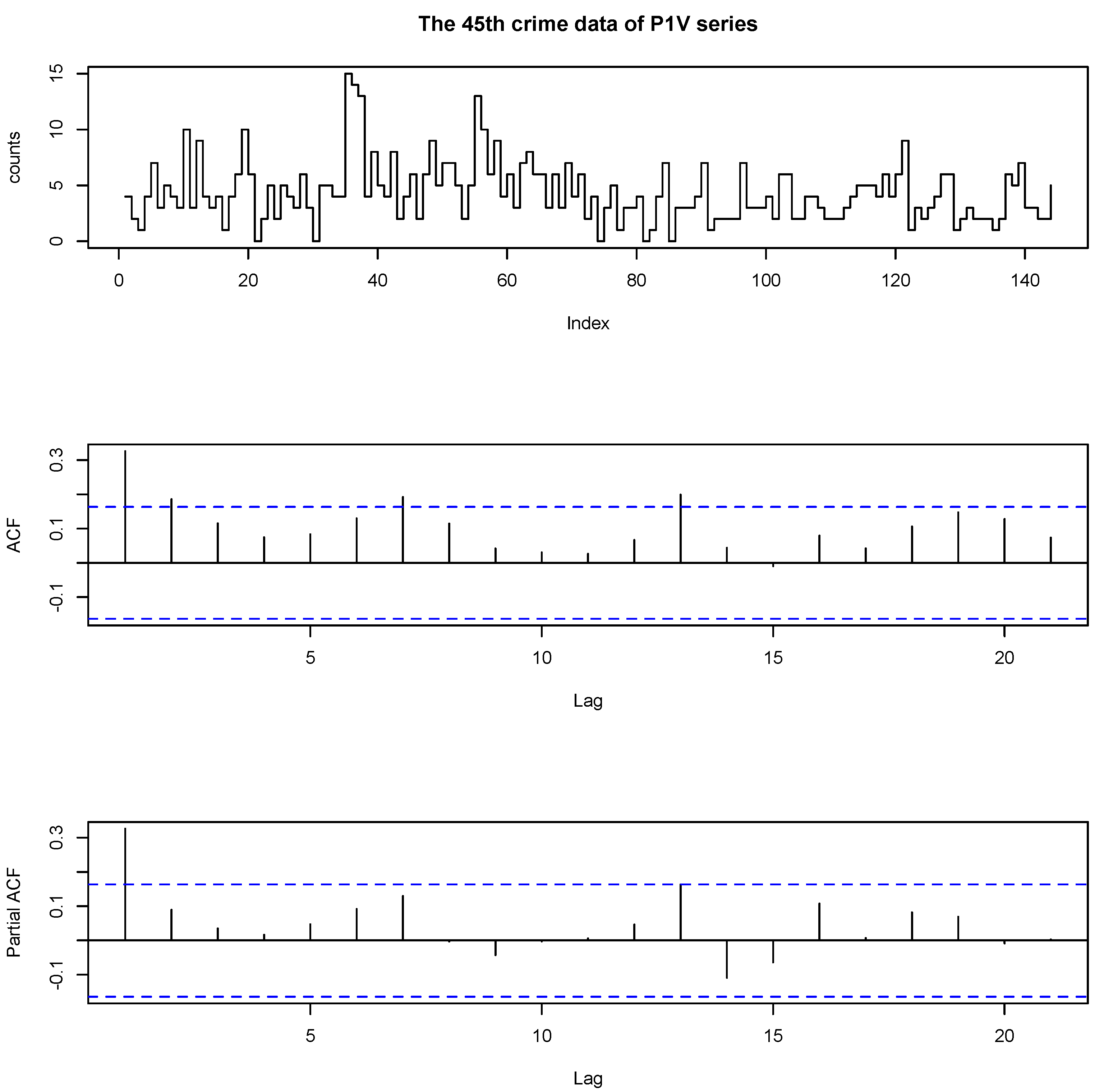
4.2.1. P1V Data
The 45th P1V (Part 1 Violent Crimes) data set contains crimes of murder, rape, robbery and other kinds; see more details in the data dictionary on the Forecasting Principles website.
Figure 1 plots the time series plot, the autocorrelation function (ACF) and the partial autocorrelation function (PACF) of 45th data of P1V series, respectively. The maximum value of the data is 15 and the minimum is 0; the mean is 4.3333; the variance is 7.4685. From the ACF plot, we found that the data are dependent. From the PACF plots, we can see that only the first sample is significant, which strongly suggests an INAR(1) model.
First, we divided the data set into two parts–the training set with the first
counting data and the prediction set with the last
data. We fit the training set by the following models: expectation thinning INAR(1) (ETINAR(1)) model in [
9], GSC thinning INAR(1) (GSCINAR(1)) model in [
10], the binomial thinning INAR(1) model and EB thinning EB-INAR(1) models with
. According to the mean and variance of P1V data, we used one of the most common settings–geometric distribution–as the distribution of the innovation in above models.
In order to compare the effectiveness of the models, we consider the following evaluation criteria: (1) AIC. (2) The mean and standard error of Pearson residual
and its related Ljung–Box statistics, where the Pearson residuals are defined as
where
and
are the estimated expectation and variance for related thinning operators, respectively. (3) Three goodness-of-fit statistics: RMS (root mean square error), MAE (mean absolute error) and MdAE (median absolute error), where the error is defined by
,
. (4) The mean of the data
on the training set calculated by the estimated results.
Next, focusing on forecasting, we generated replicates based on the training set for each model. Then we calculated the FMSE and FMAE for each model.
All results of the fitted models are given in
Table 3. There is no evidence of any correlation within the residuals of all five models, which is also supported by the Ljung–Box statistic based on 15 lags (because
). There were no significant differences for the RMS, MAE, MdAE and
values (the true mean of the 134 training set was 4.3880) of the models. In other words, no model performed the best in terms of these four criteria, so we also considered AIC. Since the CML estimator cannot be adopted in GSCINAR(1), one can only compare other criteria.
Considering the fitness on the training set, the EB-INAR(1) with has the smallest AIC, EB-INAR(1) with has almost the same AIC as . For the results on forecasting, EB-INAR(1) with has the smallest FMSE and the second smallest FMAE among all models. EB-INAR(1) with has the second smallest FMSE and the smallest FMAE. Based on these results, we conclude that EB-INAR(1) with performs better than INAR(1), ETINAR(1) and GSCINAR(1).
4.2.2. Stock Data
We analyzed another overdispersed data set of Empire District Electric Company (EDE) from the Trades and Quotes (TAQ) data set in NYSE. The data are about the number of trades in 5 min intervals between 9:45 a.m. and 4:00 p.m. in the first quarter of 2005 (3 January–31 March 2005, 61 trading days). Here we analyze a portion of the data between first to fourth trading days. As there are 75 5 min intervals per day, the sample size was T = 300.
Figure 2 plots the time series plot, the ACF and the PACF of the EDE series. The maximum value of the data is 25 and the minimum is 0; the mean is 4.6933; and the variance is 14.1665. It seems that the series is not completely stationary with several outliers or influential observations based on the time series plot. Zhu et al. [
18] analyzed the Poisson autoregression for the stock transaction data with extreme values, which can be considered in the current setting. From the ACF plot, we found that the data are dependent. From the PACF plots, we can see that only the first sample is significant, which strongly suggests an INAR(1) model. We used the same procedures and criteria as before. We used the geometric distribution as the distribution of the innovation in above models.
First divide the data set into two parts–the training set with the first
data and the prediction set with the last
data. All results of the fitted models are given in
Table 4. Among all models, EB-INAR(1) with
has the smallest AIC, and there is no evidence of any correlation within the residuals of all five models, which is also supported by the Ljung–Box statistic based on 15 lags. There are no significant differences for the RMS, MAE, MdAE and
values (the true mean of the 270 training set was 4.3407) of all considered models. For the results of prediction, EB-INAR(1) with
has the smallest FMSE and FMAE among all models. Based on the above results, we conclude that EB-INAR(1) with
performs best for this data set.
4.3. Underdispersed Case
The 11th FAMVIOL data set contains the crimes of family violence, which can also be obtained from the Forecasting Principles website.
Figure 3 plots the time series plot, the ACF and the PACF of the 11th data set of FAMVIOL series. The maximum value of the data is 3 and the minimum is 0; the mean is 0.4027; and the variance is 0.3820. We use the procedures and criteria in
Section 4.2.1 to compare different models. According to the mean and the variance of FAMVIOL data, we use one of the most common settings-Poisson distribution as the distribution of the innovation in above models.
All results of the fitted models are given in
Table 5. There is no evidence of any correlation within the residuals of all five models, which is also supported by the Ljung–Box statistic based on 15 lags. There are no significant differences about the criteria on the fitness and forecasting of all models. ETINAR(1) with the biggest AIC, performed the worst in these models.
Now let us have a brief summary. For the P1V data and stock data, which are overdispersed with slightly high-count data, the EB-INAR(1) of is obviously better than . For the FAMVIOL data, which is underdispersed with small-count data, the EB-INAR(1) with is also competitive.


