1. Introduction
Since the 1980s, a dynamical systems approach to nonequilibrium phenomena has been developed, side by side with the increase of computing power and the ability to perform Molecular Dynamics (MD) simulations. Classical MD consists of algorithms meant to solve Newton’s dynamical equations for interacting particle systems, that may be subjected to external fields. Such investigations result quite informative and practically useful, when quantum effects are irrelevant or negligible, which is the case of fluids under standard conditions.
Provided no dissipative forces are present, one speaks of equilibrium MD, which is widely used together with statistical mechanical relations, in order to compute: rheological properties, polymers behaviours in porous media, defects in crystals, friction between surfaces, formation of atomic clusters, features of biological macromolecules, formation of drugs, etc. The results are most satisfactory, and, in practice, difficulties only arise if the interatomic forces are too complicated to properly implement, if the required number of simulated particles is too large, or the simulation times too long. In fact, the statistical relations connecting microscopic dynamical quantities to macroscopic properties provide quite an accurate and complete description of material objects. Therefore, MD is used to properly interpret results of experiments, and even in place of expensive or impossible experiments. For instance, MD may illustrate the formation of crystal defects, the propagation of fracture fronts inside solids, and the thermal dilation of nuclear fuel pellets inside a nuclear reactor, just to mention a few examples. The relevant literature is enormous, and dates back to early days of electronic computers, the Fermi–Pasta–Ulam–Tsingou problem being a forerunner that opened the way to an incredible number of mathematical, computational and physical advances [
1,
2]; see e.g., the books [
3,
4,
5,
6,
7].
When the system of interest is driven away from equilibrium by external forces that continually feed energy in it and, at the same time, it is in contact with some environment that removes energy from it, a nonequilibrium steady state may be reached. The question is how to effectively model the typically very large environment [
8]. Various methods have been developed for that. In particular, researchers introduced “synthetic forces” meant to efficiently represent the effect of a bath or reservoir on the property of interest for the system of interest, without simulating the atoms of the environment. Nonequilibrium MD (NEMD) was thus born, focusing on specific quantities of specific systems [
6,
9].
The term “synthetic” means that such forces do not exist in nature; they merely constitute a
“mathematical device used to transform a difficult boundary condition problem, the flow of heat in a system bounded by walls maintained at differing temperatures, into a much simpler mechanical problem”, cf. the Introduction of Ref. [
6]. In practice, the synthetic forces constrain in various ways the dynamics of particle systems fixing, for instance, the average of the fluctuating kinetic temperature. Such an approach is so successful that the corresponding algorithms are now provided as default routines of MD packages [
10,
11].
If the constraints are holonomic and the other forces conservative, the resulting equations of motion are Hamiltonian [
12]; otherwise they are non-Hamiltonian and, in particular, they are dissipative, in the sense that on average they contract phase space volumes, although they remain time reversal invariant [
6]. Consequently, from the angle of dynamical systems, their invariant measures are singular with respect to the Lebesgue measure. This approach may sound odd, if one expects all features of the dynamics to be derived from a Hamiltonian, but it simply replicates the usual construction of effective models, that bridge the gap between different levels of descriptions of natural phenomena, [
13]. For instance, the Boltzmann equation and the Langevin equation alter the Hamiltonian dynamics to the point that it becomes irreversible and not deterministic; at the same time their success and foundational importance is not questionable. Justifications of the NEMD approach, within its specific realm, have been provided, demonstrating, for instance, that it properly computes transport coefficients [
6]. Moreover, NEMD has been shown to provide a route to extend to dissipative dynamics the theory of equivalence of ensembles, as well as Khinchin’s approach to ergodic theory in physics [
6,
9,
14,
15,
16].
The point is the following: no mathematical model spans all space and time scales of interest for a given material object: a model is acceptable when it describes a certain set of properties that are observable within given space and time scales. Of course, the wider the range of applicability of the model, the better it is. In this respect, classical Hamiltonian dynamics is no exception. It constitutes a tremendously effective microscopic model for a vast variety of non-dissipative phenomena, but dissipation makes its use problematic, cf. recent investigations on kinetic theory [
17,
18]. Analogously, models derived within the framework of NEMD, such as Gaussian thermostatted dynamics, or Nosé–Hoover thermostatted dynamics can be accepted as valid models of certain phenomena. The question is how many aspects of a given phenomenon are properly described by NEMD models. As generally true in physics, interesting results and relations can be derived in uncharted territories, but only experience can eventually confirm or refute their validity.
As a matter of fact, NEMD has become popular for its effectiveness in computing transport coefficients, such as the viscosity of a fluid [
6]. It was also realized that such coefficients can be obtained from dynamical systems properties such as the sum of Lyapunov exponents or, under special conditions, just from the sum of the largest and of the smallest exponent [
6]. In turn,
, the opposite of the phase space volumes variation rate
, which turns out to be proportional to the thermostatting (fictitious or synthetic) term may also be proportional to the entropy production
when thermodynamics applies, see e.g., Ref. [
19]. (A similar idea had previously been independently investigated by Andrej, who followed a different approach [
20]). This idea became very popular when Evans, Cohen and Morriss applied a representation of SRB measures to the fluctuations of
in a Gaussian isoenergetic shearing system [
21], as in that case such a quantity equals the entropy production, when local thermodynamic equilibrium (LTE) holds. That paper derived and tested the Fluctuation Relation (FR), one of the rare exact relations for nonequilibrium thermodynamics based on microscopic deterministic dynamics. For a time reversal invariant model of shearing fluids, the FR states that positive values of the energy dissipation, are exponentially more probable than their opposite. This was interpreted as an explanation of the second law of thermodynamics, and motivated a flurry of activity. Moreover, it led various authors to identify the entropy production with the phase space contraction [
22,
23].
Although
is relatively easy to handle in dynamical systems theory, it was pointed out that its identification with
is only justified in a limited set of cases [
24,
25]. Furthermore, in time dependent settings and in presence of fluctuations, the connection of
with physically measurable properties results rather loose. It was then shown that the physically relevant quantity in the cases described by NEMD is the so called Dissipation Function
, which preserves the meaning of energy dissipation rate even when LTE is violated, and thermodynamic quantities such as
do not exist. Only in a few cases
equals
, although steady state averages of
and
may be simply related to each other.
Later
became the basis for a general response theory, in which it plays a role as fundamental for nonequilibrium states as thermodynamic potentials do for equilibrium states. It can be used to solve in terms of physically relevant quantities the Liouville equation and, consequently, to investigate the exact average response of the observables of ensembles of systems. Furthermore,
can be used to provide conditions for the evolution of single systems, [
26,
27]. (This should be contrasted with the fact that almost invariably response of systems to perturbations is given in terms of ensembles, and that a comparatively limited amount of works have tackled response beyond its linear approximations). Most importantly, these results are expressed in terms of a physically measurable quantity, rather than in terms of an abstract phase space quantity.
Unfortunately, it is rather complicated to thoroughly investigate the properties of the dissipation function in realistic particle models. Therefore, we consider mathematically amenable dynamical systems, even if their physical relevance may be limited, as often and successfully done in statistical physics, with the purpose of illustrating aspects of the relation between dynamics and thermodynamics; think for example of Helmoltz’s celebrated theorem [
28]. Recently, Qian, Wang and Yi have also followed this route, scrutinizing a number of interesting examples and investigating them in terms of the phase space contraction rate
[
29]. The result is a set of intriguing relations between different dynamical quantities and formal thermodynamic quantities. In consideration of the fact that small systems, hence non-thermodynamic fluctuating quantities, as well as time dependent situations are ever more relevant in science and technology, we are going to perform a similar analysis within the dissipation function formalism.
This paper is organized as follows.
Section 2 summarizes the theory of the Dissipation Function, also analyzing exactly solvable examples and numerical simulations.
Section 3 compares linear Green–Kubo and exact response.
Section 4 follows in part Ref. [
29], using
rather than
. The two approaches appear as largely equivalent, since they both arise from the solution of the Liouville equation.
Section 5 explicitly solves the cases of simple attractors, and of small dissipation, in the sense of small
.
Section 6 discusses with examples the conditions under which the exact response theory based on
holds, showing that
has to be continuous at least, and that the initial phase space probability density
has to be positive in all the space that can be explored by the dynamics. This condition, called ergodic consistency [
30] is reminiscent, but weaker than the requirement that initial and asymptotic measure be absolutely continuous with respect to each other, also called equivalence [
31]. If that is not the case, modifications to the response formulae are required [
32].
Finally,
Section 7 summarises our work, highlighting two points in particular: investigating simple systems allows us to understand properties of
that are not immediately evident in realistic particle systems; on the other hand we propose a kind of thermodynamic formalism for the analysis of dynamical systems, cf. Ref. [
33], that is based on the language of nonequilibrium, rather than of equilibrium, statistical mechanics.
Section 7 also stresses the role of
as the energy dissipation, in the case of interacting particle systems.
Remark: one of the anonymous referees pointed out that the scope of our investigation can be substantially extended, because:
“most quantum transport effects could be recast into a classical simulation picture of nonlocal collisions”, cf. [
34,
35].
2. The Dissipation Function
Consider a system whose “microscopic” state is described by a dynamical system
Let (
1) generate a flow on
, i.e., a map
, such that
is the solution of (
1) at time
t with initial condition
. Further properties of
and
will be specified when needed. Let
be a probability measure absolutely continuous w.r.t. the Lebesgue measure
, and denote by
its density function, i.e.,
. A measure
is called invariant if
for any measurable set
and for all
. If
is not invariant, it evolves under the dynamics, so that at time
t it is expressed by
. Provided the flow is sufficiently smooth,
is absolutely continuous, and has density
that satisfies [
27]:
where
is the dissipation function, defined by:
and
denotes the phase space variation rate. Its negative,
, is called phase space contraction rate. In the case the dynamical systems represents an equilibrium system, with equilibrium distribution
, so that
, the dissipation function identically vanishes,
. It is obviously true also the converse: if
then
is an invariant density. In the general case, the solution of (
2), is given by [
27]:
where, for every phase function
we use the notation
Given any observable
, we define its ensemble average according to the measure
as
Under suitable conditions, discussed in
Section 6, this average can be computed using the dissipation function as follows [
27]:
Equation (
8) gives the response of an equilibrium system, characterized by the distribution
, invariant for the dynamics
, which at time 0 is perturbed so that its dynamics becomes Equation (
1). The measure
is not invariant under the new dynamics, hence it evolves together with the averages representing the observables. At time
t the initial measure has turned into
, and the initial average
into
.
In the long time limit, the response may be given by a non equilibrium invariant distribution. As (
8) is exact, the existence of such an asymptotic average is equivalent, as a necessary and sufficient condition called
T-mixing, to the convergence of the following limit:
for any observable
. A sufficient condition for the existence of
is [
26]:
A further useful asymptotic property is obtained by considering two observables
and
. In this case, we say that the system is
T-mixing [
26] if
We observe that setting
in (
11) we obtain a weak form of
-mixing, namely
given that one has, cf.
Section 6 and [
27]:
Obviously, T-mixing implies weak -mixing. We observe that these properties may hold on a specific set of observables for a given but not for other initial distributions.
A fundamental difference between
T-mixing and the mixing property of standard ergodic theory is that
T-mixing concerns a the decay of correlations w.r.t. the initial state
, hence it may properly describe the irreversible relaxation of a given system to a stationary state. Mixing, instead, corresponds to a decay of correlations within a given steady state, since it refers to an invariant measure [
5]. We refer to Refs. [
5,
27] for a broader discussion of these issues.
2.1. Examples
The physical meaning of the Dissipation Function can be appreciated by considering some special choices of vector field
, and of initial probability density
. First, consider the NEMD systems for which
has been introduced, to see that in such cases it is directly related to the instantaneous dissipative flux. The simplest of these systems have the following equations of motion:
where
collectively represents all coordinates
q and momenta
p of the
N particles, and
is the external driving field, coupled to the particles via the “charges’’
and
. The term
is a Lagrange multiplier meant to implement some constraint, so that the system reaches a steady state despite the driving field. In the NEMD literature
is said to implement a deterministic, time reversible thermostat [
6]. If this thermostat is set to 0, one obtains the adiabatic equations of motion:
which imply a continuous growth of energy. Then, one must assume that the support of
is densely explored by a single equilibrium trajectory [
30].
Denoting by
the internal interaction potential energy of the
N particles, the dissipative flux,
, is obtained from the time derivative of the internal energy
under the dynamics (
15), which represents how much energy has to be dissipated in order to keep the steady state. The result is:
where
V is the volume of the system.
Consider a few common examples.
2.1.1. Microcanonical Ensemble
For the isoenergetic dynamics, in which the internal energy is conserved, i.e.,
is fixed and
, the equilibrium ensemble
is microcanonical. Therefore, for an equilibrium Hamiltonian
N particle system in
d dimensions, one has [
30]:
where
K is the kinetic energy of the
N particles, while
as in the original paper [
36]. Then, one may write:
As even the
correction in Equation (
18) is proportional to
, one observes that in this case both
and
are proportional to the rate of energy dissipation (
17).
2.1.2. Gaussian Isokinetic System
In this case the kinetic energy
K is fixed, and one may formally write
, if also the center of mass is fixed, to prevent contributions from drift, so that:
In turn,
is still expressed by (
18), with a different
term. In this case,
writes:
where
Q is the normalization constant. The result for the dissipation function is:
where the bar over the observables denotes time average. Combining this with Equations (
18) and (
19), one obtains
where
is the entropy production, if local thermodynamic equilibrium is verified. We observe that
and
differ by a term proportional to the fluctuating
. If these fluctuations average to zero, the averages of
and
coincide, however, depending on how the respective fluctuations are distributed, various relations may apply to one and not to the other. For instance, the steady state fluctuation relation may hold for
but not for
, [
37,
38].
2.1.3. Nosé-Hoover Thermostat
In this case, there is one extra equation to be added to the equations of motion (
14):
where
sets the relaxation time scale of the thermostat, and
T is the imposed average temperature. Then, we may write:
and for unperturbed Hamiltonian dynamics, one may write:
In this case,
is given by
where
M is the normalization. It follows that:
which implies:
We conclude that for equilibrium Hamiltonian dynamics, the driven nonequilibrium evolution is characterized by the dissipation function, which equals the entropy production, in case local thermodynamic equilibrium holds. Additionally, in this case and differ by a term proportional to , and the same remarks concluding the previous subsection equally apply.
2.1.4. Canonical Ensemble for Generic Dynamics
The canonical ensemble describes the equilibrium state of a Hamiltonian particle systems in contact with a heat bath at temperature
, with which it can exchange energy but not matter. Here, we consider a general case in which the vector field
is not necessarily Hamiltonian, but there still is an energy function
H. In addition, we assume that the initial distribution has the same form of the canonical Gibbs density:
being the normalization constant. Then, the Dissipation Function reads:
where we use the notation
. The Dissipation Function
is not necessarily zero, in this case, and the density evolves as follows, cf. (
5):
where:
. In the case of Hamiltonian dynamics,
,
where
is a symplectic matrix, we have
and
. Thus, in the equilibrium canonical ensemble, where (
26) is invariant and the phase space volume is conserved, the dissipation function is identically zero
.
The extended canonical equilibrium distribution of the Nosé–Hoover thermostatted system can be framed in this way: its dynamics includes a degree of freedom
that represents the heat bath, and system plus bath constitute a canonical equilibrium state. For instance, consider a system made of
N identical noninteracting one-dimensional oscillators in contact with a bath at temperature
T, implemented by a single Nosé–Hoover thermostat. This thermostat introduces an indirect coupling among the oscillators, which however does not represent a proper interaction leading to LTE. We illustrate these facts considering both linear and nonlinear oscillators, i.e., potential energies
, with
and
. The equations of motion are
where
T is the target kinetic energy per particle,
is the kinetic energy per particle, and
the relaxation time. In order to elucidate the non-thermodynamic nature of the model (
28), we simulated a system of
oscillators in the linear case,
, with
,
,
and
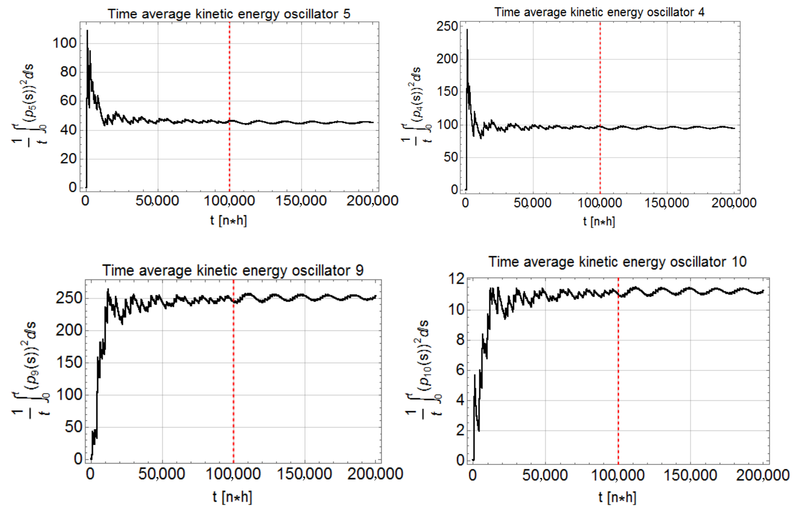
. As expected because of the improper particles coupling expressed by
, we observe no equipartition; cf.
Figure 1, which shows that the time average
of the kinetic energies of single particles substantially change with their label
i, while the time average
of the total is equal to
T within numerical errors. The same happens also with
.
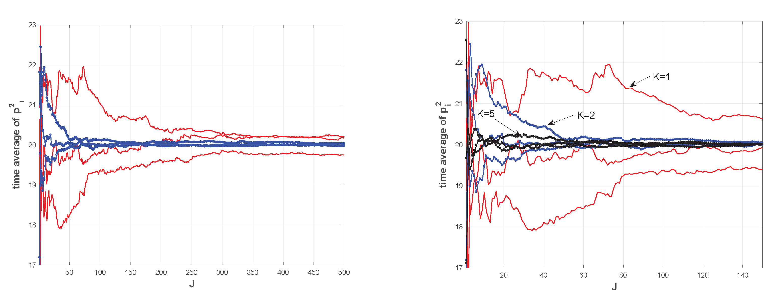
To promote LTE in this system, we introduce nearest neighbour interactions as:
in place of the second of (
28), taking
as the coupling strength, and
,
as boundary conditions. Unlike the previous non-interacting model, the linear (
) and nonlinear (
) cases behave in a different way. While still absent in the linear case, equipartition is established with the cubic local field.
Figure 2 shows the time averages
of the kinetic energies of some particles sampled form a long trajectory of the coupled system with
. We consider the cases with
in order to make evident the role of the coupling. These simulations show that increasing the particles coupling
k speeds up the equipartition process. Changing the oscillators frequency, instead, has no effect on equipartition, cf.
Figure 1.
Now, focusing on the energy
of the system of oscillators alone, i.e., without the bath, and taking
as
in order to define a kind of reduced dissipation function for the dynamics with the bath, one obtains:
which is not identically zero even in the equilibrium state. There is no immediate physical interpretation of the quantity
, but it clearly shows that, in this framework, the thermostat has to be included to properly speak of equilibrium.
2.1.5. Hamiltonian and Gradient Vector Field with Canonical and Gaussian
In the case of Hamiltonian dynamics perturbed by a gradient term [
39]:
where the unperturbed equilibrium density should be chosen consistently with the constraints that remain in place when the perturbation is switched on, in order to implement the above-mentioned ergodic consistency condition. For instance, if the system temperature remains fixed, one may take the canonical distribution,
, that implies:
being the Laplacian of
L. One observes that
only depends on
L if
is orthogonal to
. If
is in addition a Hamiltonian perturbation, the perturbed steady state remains equal to the unperturbed equilibrium. Now, taking an initial uncorrelated Gaussian distribution:
one obtains:
being the entries of
. Again, a Hamiltonian perturbation such that
implies that the Gaussian (
32) is invariant under the dynamics. These two examples constitute elementary warnings against too quick thermodynamic interpretations of generic particle systems, much as it may be interesting in certain circumstances [
40].
2.2. The Dissipation Function and the Phase Space Contraction Rate
The Dissipation Function satisfies the Non Equilibrium Partition identity [
27]:
Using Jensen inequality, we can also write:
obtaining:
in accordance with both our physical intuition on the dissipation of energy in macroscopic systems and with the interpretation of this quantity as a Kullback–Leibler divergence between the initial and the evolved probability distribution in phase space [
27].
One motivation to derive relations like these, see e.g., Refs. [
27,
30] where various others are derived, resides in the fact that they are only based on the dynamics and on the initial probability distribution, whatever phenomenon they represent, hence they hold very generally. At the same time, this also means that blind thermodynamic interpretations are to be avoided, although no difficulty arises from a purely dynamical systems standpoint.
The distinction between the dissipation function and the phase space contraction rate
becomes particularly evident when considering particle systems. In fact, the steady state phase space average of
equals the steady state entropy production of certain NEMD models [
6,
19], and it can be expressed as:
being the corresponding invariant measure, and
the steady state entropy production or the energy dissipation. On these grounds, Gallavotti and Cohen proposed
as the steady state definition of entropy production tout court, [
41], followed by Ruelle [
23]. Earlier, a similar idea had been contemplated by Andrey [
20], who referred to the variation in time of the Gibbs entropy. The Gibbs entropy, however, is not directly related, in general, to the entropy of a nonequilbrium system [
42,
43,
44]. (Note: this statement does not concern the formally analogous definition of entropy common in the theory of stochastic processes, since they are not defined in phase space but in the space of observables.) Therefore,
cannot be directly related, in general, to the entropy production, when considering time dependent states or steady state fluctuations, cf.
Section 2.1 and Refs. [
27,
30,
38].
On the other hand, it is interesting to investigate both
and
as properties of dynamical systems, in a kind of extension of the thermodynamic formalism [
33], that refers the non-equilibrium language.
Given an initial absolutely continuous probability measure
on the phase space
, and letting
be the evolution of
at time
t, the corresponding average of the dissipation function is:
which in the case of a uniform density
yields:
In this case, even
does not need to represent any entropy production rate: the equilibrium dynamics would have at least to be phase space volumes preserving, for
to be related to the dissipation of energy [
30]. Using Equation (
8) and the fact that
, we may also write:
In the case of a generic probability density
, the exact response formula (
8) and (
40) yield:
which quantifies the difference between the mean phase space contraction rate and the energy dissipation in time. In the case
-mixing, Equation (
9), holds,
t can be replaced by
∞ in (
41), obtaining the asymptotic difference between the two quantities:
From the definition of dissipation function
, i.e., Equation (
3) with
, one also observes that
Therefore, the time integrated difference of
and
merely amounts to a boundary term:
which, however, may bear noticeably affect the statistic of fluctuations: the distribution of such boundary terms may, for instance, imply the validity of the FR for
and not for
, cf. [
37,
38,
45].
3. Exact Response and GK Formalism
In this section, we compare the classical linear response theory, or Green–Kubo formalism, with the exact response represented by Equation (
8). Consider a perturbed vector field
where
may or may not be small. Then, the Dissipation Function can be written as:
and the evolution of a probability density
is given by
where
denotes the flow of the vector field
. Thus, the exact response Equation (
8) reads
In case
derives from a Hamiltonian
, the unperturbed dynamics preserves phase space volumes, and one can write:
where
is the Liouvillean corresponding to
and
denotes the associated Poisson brackets. Then, we may define the perturbation operator
as:
so that the (total) dissipation function can be written as:
Substituting (
51) in (
48) yields:
and in case the initial distribution
is the equilibrium state of the unperturbed system, so that
, one obtains:
Provided the response Equation (
8) applies, the formulae (
52) and (
53) for the evolution of phase space averages are both exact: there is no assumption on the size of
and no approximation has been made. An approximate formula can be obtained in the small-
limit, starting from Equation (
47), by truncating to first order the exponential expansion, and recalling that
. This yields:
where the tilde symbol stresses that this is but an approximation of the probability density at time
t, which is not guaranteed to be a probability density itself. Nevertheless, multiplying (
54) by
and integrating over the phase space, one gets:
In order to keep the truncation error bounded in time, one may assume that the time integral exists. For instance,
maybe of order
, which is reminiscent of the
-mixing condition. The difference between the exact response formula, (
48), and the approximate one, (
55), amounts to:
that, in general, does not vanish, and may grow large in time.
May the difference of responses Equation (
56) become negligible, in some limit? Applying the transformation
to the second integrand of (
56), one obtains:
where
since we are dealing with Hamiltonian dynamics–being
the Jacobian determinant. Thus, Equation (
56) can be rewritten as:
For every finite
t, this quantity vanishes in the
limit but, unlike the case of the Green–Kubo theory of linear response, the flow used in (
58) is the perturbed one,
, not the unperturbed
.
As a matter of fact, the success of the Green–Kubo theory is based on its ability to compute the response by averaging with respect to the equilibrium ensemble for the unperturbed dynamics, and by simulating such an unperturbed dynamics [
46]. The procedure, illustrated in many textbooks, including [
46,
47], uses the canonical ensemble for the unperturbed Hamiltonian
,
, and assumes that the parameter
is the magnitude of and external force
. Within the framework of NEMD and Equation (
14), one starts from the unthermostatted,
situation. Without loss of generality, the external driving
can be written as a scalar quantity, since its direction can be embedded in the coefficients
and
. Then, the unthermostatted perturbed equations are derived from a Hamiltonian,
. Writing
to distinguish configuration from momenta,
is obtained deriving
:
and the following holds:
In this case, one has:
which equals Equation (
16), and shows again that
, not
, represents that energy dissipation rate. Now, following the Green–Kubo approach [
46,
47], which rests on the fact that
one may use the unperturbed dynamics, and eventually write:
to first order in
, for a generic observable
. The function
is called the response function. In particular, the difference in (
56) between exact and linear response can be expressed as:
That the full dynamics
can be replaced by the equilibrium dynamics
is a far from trivial fact. In fact, van Kampen raised one of the best known objections to this theory, based on the observation that particles dynamics are typically chaotic [
48]. He maintained that while there is no doubt that linear response works in practice, the derivations a la Green and Kubo do not explain why. He stated that:
“Linear response theory does provide expressions for the phenomenological coefficients, but I assert that it arrives at these expressions by a mathematical exercise, rather than by describing the actual mechanism which is responsible for the response” [
48]. It fact, to justify the Green–Kubo calculation, one must invoke non trivial ingredients, such as the large value of
N, which makes the perturbation per degree of freedom negligible, and the mingling of contrasting contributions operated by chaos, see e.g., [
45,
49,
50]. As such conditions actually hold in macroscopic particles systems under quite variegated conditions, the Green–Kubo reasoning explains the success of linear response.
3.1. Exact Response and GK Formalism: Example 1
Consider a particle in a two-dimensional space, whose unperturbed Hamiltonian is
. Take the canonical ensemble
as the initial distribution. Introduce an external field with Hamiltonian
, as a perturbation to obtain
. The corresponding equations of motion are:
with the dissipation function
in which the momentum in
x-direction plays the role of internal dissipative flux with
E the corresponding thermodynamic force, i.e.,
and
. Note that the present example is an instance of the adiabatic system (
15), in which
and
,
, see (
59). Sticking to the notation of
Section 2.1 in the following we denote by
the phase space points and observe that the solution of (
66) with initial condition
gives
and
.
Then, thanks to Equation (
5), we compute the time evolution of the probability distribution function
starting from the integrated dissipation function:
obtaining
Following the discussion in
Section 3, we expand the exponential in the limit of small external field
E, and we neglect the terms of order higher than linear in
E, to obtain the linear response for the evolving density:
The difference between exact and linear response can be further clarified by looking at the Liouville equation for
and proceeding a la Green–Kubo. Let us start introducing the Liouville operator of the perturbed system:
where
corresponds to the unperturbed system and
corresponds to the perturbation. Splitting the evolving ensemble distribution function as:
the Liouville equation takes the form:
Recalling that the equilibrium distribution
is invariant under the unperturbed dynamics—so that
—we obtain the evolution equation for the deviation
:
Then, assuming that
is negligible w.r.t. the other terms, we arrive at:
Since
, the Equation (
67) can be rewritten as
where
,
and
, according to standard notation. The solution to the evolution equation for the variation of the ensemble distribution function, is given by:
where we have used the fact that the external perturbation is not time dependent.
Let us now compute the phase space average of an observable
, using
. We can write:
noting that
is the flow of the unperturbed dynamics. As an example, take
, and compute its time evolving linear response. Since
and
, we have:
Now, denoting by
the flow of the perturbed system, and recalling that
and
, the exact response formula (
8) yields:
For such an observable, linear and exact response coincide. In general, we have:
For an analytic observable that do not depend on
and
, we have:
assuming that
is an analytic function, and denoting by
the
th partial derivative of
with respect to
, at fixed
. The difference between the exact and the linear response would read:
Depending on the particular functional form of this quantity may grow rapidly or less rapidly with t and, as long as exists at all t, this difference at fixed t goes to 0 as .
3.2. Exact Response and GK Formalism: Example 2
Let the unperturbed Hamiltonian correspond to a harmonic oscillator
, and let the perturbation take the form
. The equations of motion of
are:
with flow
The dissipation function with initial distribution
is given by:
since the vector field is Hamiltonian and
vanishes. Moreover, we see that
coincides with the dissipation function
of the vector filed of
, because
is the equilibrium distribution of
. Thus the exact and the linear response formulas are respectively given by:
and
Consider now
. In this case
and
are given by (
76). For
we have:
since
,
and
. The response formula (
78) gives
Analogously, the unperturbed dynamics, given by
in (
76), yields:
and from (
79)
This shows that the perturbed and unperturbed responses of the observable
coincide. If we consider the observable
, the situation is different. In the first place,
that must be multiplied by
p before taking the ensemble averages in (
78) and (
79). This gives a linear combination of monomials
, whose average with respect to
vanishes, and a non vanishing term
Thus, recalling that
, we have:
On the other hand, from (
84) with
, we obtain that
is a linear combination of
. This implies that
and, from (
79), that
, showing that the perturbed and unperturbed responses substantially differ in the case of
, unless
E is particularly small.
4. Formal Thermodynamics
Following Qian and collaborators [
29], we now obtain various new relations for the dissipation function. To this end, suppose that the system admits an energy function
,
. Let us introduce the set
in phase space, defined as follows:
and its boundary:
The set
includes all points in phase space whose energy is equal to or lower than the threshold
h, and
is its boundary, constituted by the phase points whose energy equals the threshold value. Introduce the measure of such sets w.r.t. the time evolving probability measure:
where
is a sufficiently well behaved probability density. Then, the function
where
is the characteristic function of
, plays the role of a probability density in
. Using Reynolds Transport Theorem plus the regularity of the surface
, one finds:
where
is the surface element area. This quantity can be interpreted as the measure w.r.t. the density
of the constant energy surface
. The time derivative along a trajectory of the energy function
is given by:
hence we may define a formal heat flux through the boundary
as:
If in addition, we introduce the formal temperature as the inverse of the logarithmic derivative of the constant energy volume w.r.t. the energy parameter
h:
we can relate the ensuing formal entropy production rate to the average of the dissipation function concerning the set
:
This result is readily obtained as follows:
where the equality is guaranteed by Divergence Theorem,
being the unit vector everywhere normal to the surface
, and by the identity
. Then Equations (
3) and (
5), yield:
that leads to:
Therefore, we can now write:
The first addend within the brackets can be reworked using the response formula (
8), where
restricted to
is considered like any other phase function:
while for the second contribution, we have:
Rearranging the two contributions, the first integral in Equation (
91) becomes:
and finally:
Letting
h grow in Equation (
88), these conditional averages converge to the average on
, yielding:
where (
13) has been used. This is consistent with the fact that in this model no “energy” can flow out of
, or in
from outside.
Note that such a reasoning actually does not refer to a physical flow: in the first place, it occurs in phase space, rather than in real space; furthermore the dynamics does not need to describe any physical phenomenon. Therefore, the thermodynamic interpretation of the above relations should be taken with a grain of salt [
43,
44], while it may be suggestive in the analysis of dynamical systems, analogously to the thermodynamic formalism [
33].
The Case with Constant or Slowly-Varying Volume Contraction
Assume that the probability density
is continuous with compact support
, and take
, with
,
sufficiently regular,
. Assume also that the system is
-mixing. To compute
up to
, observe that:
where
Substituting in (
96), we have:
The second integral can be computed explicitly taking
on
:
As the divergence of
equals the constant
, and
, we have:
The integral in the previous equation is, by the Divergence Theorem, equal to
Averaging
one has instead:
since to first order, our vector field has a constant phase space volumes contraction rate.
Example 1. The simplest case is obtained when the initial distribution is uniform, i.e., constant, as if the “equilibrium” vector field vanishes. In that case the integrals in (101) vanish, and Example 2. Suppose the coordinates in the initial ensemble are independent, i.e.,with being one dimensional density functions. Then,and Equation (101) can be rewritten as follows:In the special case of Gaussian marginalswe have:The simplest example can be obtained with and , , and assuming . Then, observing that the i-th component of , can be written as , Equation (105) becomes:where . In addition, recalling that and , we have:The previous result could have been obtained directly from Equation (96), noting that:Equation (107) shows that the average dissipation function diverges as , because the dynamics has the global attractor . Thus, tends to the non vanishing phase space contraction rate . That is not the case for . 5. Simple Attractors and Small Dissipation
Consider the dynamical system (
1) on a compact phase space
containing a set of attracting fixed points
with (open) basins of attraction
, such that
, modulo a set of zero Lebesgue measure. Let
be the initial probability density and
its evolution at time
t. Recalling that the basins of attraction are pairwise disjoint, for any continuous phase function
C we can write:
Taking the limit, by bounded convergence we have:
This shows that the asymptotic mean of
C is the weighted mean of the values of
C on the attracting fixed points, with weights given by the
-probability measure of the corresponding basins of attraction. In other words, the probability measure
converges weakly in time to
, with
the atomic measure on
. In this case it is easy to compute the correlation function of
A and
C w.r.t.
:
that is used to define T-mixing and, taking
, to define
T-mixing, cf. Equations (
10) and (
11). The
limit of (
110) then yields:
and, assuming that also
is continuous,
since
.
Remark 1. For , the response from a single initial condition is not unique and depends on the initial distribution . Hence, T-mixing does not hold, since it requires the long time averages to be independent of the initial condition [26]. On the other hand, ΩT-mixing holds, since it is necessary and sufficient for the convergence of the full phase space averages to their asymptotic limit, i.e., (109). Now, consider a case with small dissipation:
where
is small, and
Then, the unperturbed dynamics
preserves the volume and the initial density, since
, while the dissipation function only depends on the perturbation
:
Let the initial probability density
be positive for every
in the phase space
, a condition at times called ergodic consistency [
30]. In this case, the probability density at time
t is given by:
where
is the flow of (
113). Taking
and
, it can be shown that the difference between the evolved density and the initial one is
, in the
-dependent time interval bound by
, provided
is continuous in
. In particular, one has:
which defines the maximum magnitude of
in
. Consequently, for
:
We can use this inequality to bound from above the variation of an observable of the system at hand. For a continuous function
B, one obtains:
6. Conditions on Dynamics and Probability Density
As observed in [
27], the dissipation function can be obtained starting from the Liouville equation:
and factorizing
in the right hand side. The result is Equation (
2) with
defined as in (
3). The standard conditions of physical interest, under which this operation can be performed are the following:
the vector field should be everywhere differentiable in the phase space for to exist;
the initial density should be everywhere positive in for its logarithm to exist;
the initial density should be everywhere differentiable in for its gradient to exist.
This also guarantees that the dissipation function be continuous, which is what is used to derive Equation (
8) from Equation (
7), via Equation (
5). In the physical literature, these requirements are satisfied if (a) the condition sometimes called ergodic consistency holds [
30]—
should be the equilibrium ensemble for the dynamics subjected to the same constraints of the nonequilbrium dynamics—and if (b) the particles interactions are sufficiently regular. The effects of discontinuities can be controlled if the dynamics are piecewise regular (as in billiards), or the probability decays sufficiently fast when approaching singularities. A full mathematical treatment of these aspects is far from trivial for physically relevant particle systems, and the success of the theory can only be judged a posteriori, on a case by case basis.
At the same time, various mathematical aspects can be understood considering simple examples, that can be explicitly solved. Let us focus on simple cases in which the above conditions are violated. This is important both to delineate the range of applicability of the theory based on the dissipation function and, at the same time, to find corrections where needed.
When
is not differentiable, one may replace (
119) by its weak form, i.e.,
being the set of smooth functions with compact support in . The non-differentiability, of , however, is not the only issue. In what follows we take and with compact support and in , while is not necessarily compact.
Examples
Example 3. Consider the dynamical systemand the following initial density:that is compactly supported and non differentiable at 1 and . As the initial condition x evolves like , is given by Then, Equation (
119) does not apply, while Equation (
120) does. Indeed, the left hand side and the first term in the right hand side of (
120) are
The phase integral in the right hand side of (
120) yields:
and the corresponding time integral becomes:
Then, integrating by parts and using Leibniz’s formula in the last integral, we get:
and
Form (
124) we get
, that proves (
120).
The probability with density
converges weakly to the delta function at
, since for any continuous
, the mean value theorem yields:
for one
. Can this result be obtained via the response formula (
8)? Because
, and
, the dissipation function takes the form:
on the interval
. Hence, unlike the cases addressed so far,
does not vanish, it equals 1!
More generally, given the 1-D system
with
and
supported on any interval
, integration by parts yields:
showing that
vanishes only if some conditions, such as
or
, are verified.
In Ref. [
27], the equality
was obtained from the conservation of probability and from the interchange of the time derivative with the integration in phase space:
This exchange is legitimate under the joint continuity w.r.t.
x and
t of
and of
, which is not the case of our example. Consequently, Equation (
8) leads to the nonsensical expression:
which diverges linearly with
t, rather than converging to
, because
. This is related to the fact that
, due to the non differentiability of
. If, on the other hand, one has
with
, one obtains:
Then, taking for instance
, which can be used for analytic functions, one has:
for even
n, which correctly converges to
, and 0 for odd
n, which equals
at all times.
The role of Equation (
13) is further clarified noticing that for a finite
t one can write:
Then, assuming the
limit and the phase integration can be exchanged in Equation (
135), the previous equation yields:
where
is the time average of
. This shows that Equation (
9) requires
, i.e., that either
vanishes or changes sign in
.
On the other hand, one realizes that this is not sufficient in general. For instance, despite the correct result (
134), the blind application of Equation (
5) for the case of Equation (
121) with density
in
, yields an incorrect evolved density
. In this case, we have:
and
which implies:
that is not normalized on
. This difficulty is not related to the violation of Equation (
13), but to the fact that the support of
changes with time or, equivalently, that Equation (
5) attributes a positive probability to points outside
. An analogous, even more macroscopic, situation arises if
and
, which yields
, hence yields (
13) with non vanishing
and
. This stresses that dynamical equations and phase space must be properly chosen.
The point is that the preimages
of part of the points in
, for some
, lie outside
. In these cases, Equation (
5) requires that only the contributions of the points
x with
be included in the calculations, as discussed in Ref. [
32].
Example 4. Consider the dynamical systemthat has two asymptotically stable fixed points and , and an unstable fixed point, . Take the invariant set as the phase space of the system. The flow is given by: Assuming
, uniform on
, the dissipation function is expressed by:
, hence it changes sign in
. The evolved distribution is given by:
If, on the other hand,
, we have
that also changes sign, and the density at time
t becomes:
From (
141) and (
143) one can see that in both cases
converges weakly to
. This is correctly so because the flow vanishes at the boundaries of the phase space:
is invariant; hence the points inside
have no preimage outside
. In this case, the non-differentiability of the uniform density in
has no bearing on the theory.
Example 5. Let us consider the one-dimensional dynamical system:and denote and . This system has three fixed points: , which is asymptotically stable, and the unstable points and . We denote by the set , which is invariant, being invariant the intervals and . Integrating the differential equation, we obtain Then, expanding with respect to
,
where
. The uniform probability on
, has compact support in
. Substituting
and
in Equation (
47) yields:
This allows us to check that the probability measure
converges weakly to the delta function at
as
The linear approximation for small
can be obtained, in analogy with the Hamiltonian case, cf. (
54), by truncating the exponential in (
47):
which gives:
It can also be observed that the linear approximation at
of the exact evolved density (
147),
does not coincide with Equation (
149), but it can be obtained from Equation (
149) approximating
to first order in
x.
Given that
, the exact response of ensemble averages is given by:
that, on the basis of the previous remarks, converges to
, as
. As observed in
Section 3, the linear approximation analogous to the GK response is obtained by replacing the exact flow
with the linearized one,
, in Equation (
151).
Now, let
A and
B be smooth functions, and
a probability density with compact support
K in
, containing
in its interior, for instance
. In order to check
T-mixing, see (
11), let us write:
which follows from the uniform convergence of
to 0, from the boundedness of
A and
B in any compact set and from the continuity of
A. This proves the T-mixing property (
11) for the present example. The same reasoning shows that the system is also
-mixing.
Example 6. Consider the one-dimensional dynamical system:that is the time reversed version of (144). The point is now unstable, while and are stable, and is invariant. The flow is expressed by:where . The ϵ expansion at has an error that grows without limit as t increases, which shows the unsuitability of the linear response. In this case, always assuming in , Equation (47) yieldsbeing and , since and . Observe that while for as . Thus the measure converges weakly to . Example 7. Let us considerand assume the invariant interval as the phase space. For the fixed points are , and . For , the point 0 is unstable, while and 1 are stable. The opposite holds for . For , all the points are fixed. The flow is given by:Taking the initial uniform distribution on , being , the evolved density is:For the distribution converges to , while for the limit is . The response isOnce again, the linear response approach is scarcely interesting. 7. Concluding Remarks
In this paper we have reviewed the developments that led from nonequilbrium molecular dynamics (NEMD) to the fluctuation relations (FR) and to the exact response theory, which develops the previous formalism based on the so-called Transient Time Correlation Function [
6]. Within this framework, some authors have adopted the phase space contraction rate
as a definition of the steady state entropy production rate
[
23,
41], after
and
had been observed to be proportional to each other, in the original paper on fluctuations relations [
36]. That paper dealt with the Gaussian thermostatted iso-energetic model of a shearing fluid known as SLLOD. In that case, the steady phase space contraction and entropy production rates could indeed be directly related to each other, something that in NEMD models had already been pointed earlier [
19,
51,
52]. Mostly the interest had been on steady state state averages of such quantities. It was then realized that such an identification is justified only for steady state averages of certain NEMD models and that, in general, fluctuations require
to be distinguished from the energy dissipation rate [
24,
25,
53]. At the same time, the function that represents energy dissipation in molecular dynamics has been identified as the dissipation function
, the function that obeys the FR. For the transient FR this happens quite generally; for the steady state FR it is required that correlations w.r.t. the initial distribution do not grow too fast, something implied by the T-mixing condition [
26].
Through a number of examples, including NEMD models as well as simple exactly solvable models, we have illustrated these facts and how the exact response formula, based on , applies. In particular we have analyzed the relation between and , noting that in the analysis of generic dynamical systems the two quantities are by and large equivalent, while in the case of particle systems the first corresponds to a real observable. We have then compared the exact response formula with the one of the Green-Kubo linear theory, quantifying their difference, that typically grows with the size of the perturbation and of time, but also showing that in some simple case they yield the same result.
We have then investigated “formal thermodynamics’’ along the lines of Ref. [
29], introducing a formal temperature and a formal energy flow, and using
instead of
as a notion of formal entropy production rate. Analogously to earlier works, e.g., Refs. [
54,
55,
56], this means that the phase space is treated as real space, and its different regions as different locations in real space. Clearly, the
-dimensional phase space of an
N particle system in
d dimensions and the phase points that flow in it are totally different from the
-dimensional real space and the particles that flow through it [
43,
44]. (A point in phase space has no extension nor “inertia’’, it does not interact with other points, and it equally represents the microstate of a large or small system. Any other point represents another system that can be arbitrarily close or far from it. A particle in real space has a finite extension, interacts with nearby particles, and follows Newton’s laws with its inertia. Just this has numerous consequences. For instance, while the Gibbs entropy represents thermodynamic entropy only at equilibrium, the Boltzmann entropy works also in time dependent situations, Refs. [
44,
57]). Therefore, in general, a direct identification of flows and related quantities in phase space with their physical counterparts is not possible. Nevertheless, this analysis is reminiscent of the thermodynamic formalism, which is important for dynamical systems in general [
33]. Furthermore, it may find direct physical application in systems of non-interacting particles, for which the factorization of the phase space distributions makes phase space and real space almost the same. Such systems may not behave thermodynamically, but they are of greater and greater interest in e.g., bio- and nano-technology (cf. transport in highly confining media), for photons in optical wave-guides or random media, for cold atoms etc.
Finally, we have observed that the exact response formula (
8), mainly rests on the regularity of the vector fields, and on the ergodic consistency of the initial distribution, which ensure the regularity of the dissipation function as well. These mathematical conditions need further scrutiny, in more realistic cases, but are relatively minimal, hence hint at a wide applicability of the theory. The investigation of physical applications of this theory is just at the beginning; many are indeed the cases in which perturbations cannot be taken as small compared to the reference signals; they range from nano-technology to geophysical and even astrophysical phenomena [
58].


