Day and Night Changes of Cardiovascular Complexity: A Multi-Fractal Multi-Scale Analysis


Abstract
:1. Introduction
2. Materials and Methods
2.1. Subjects and Data Collection
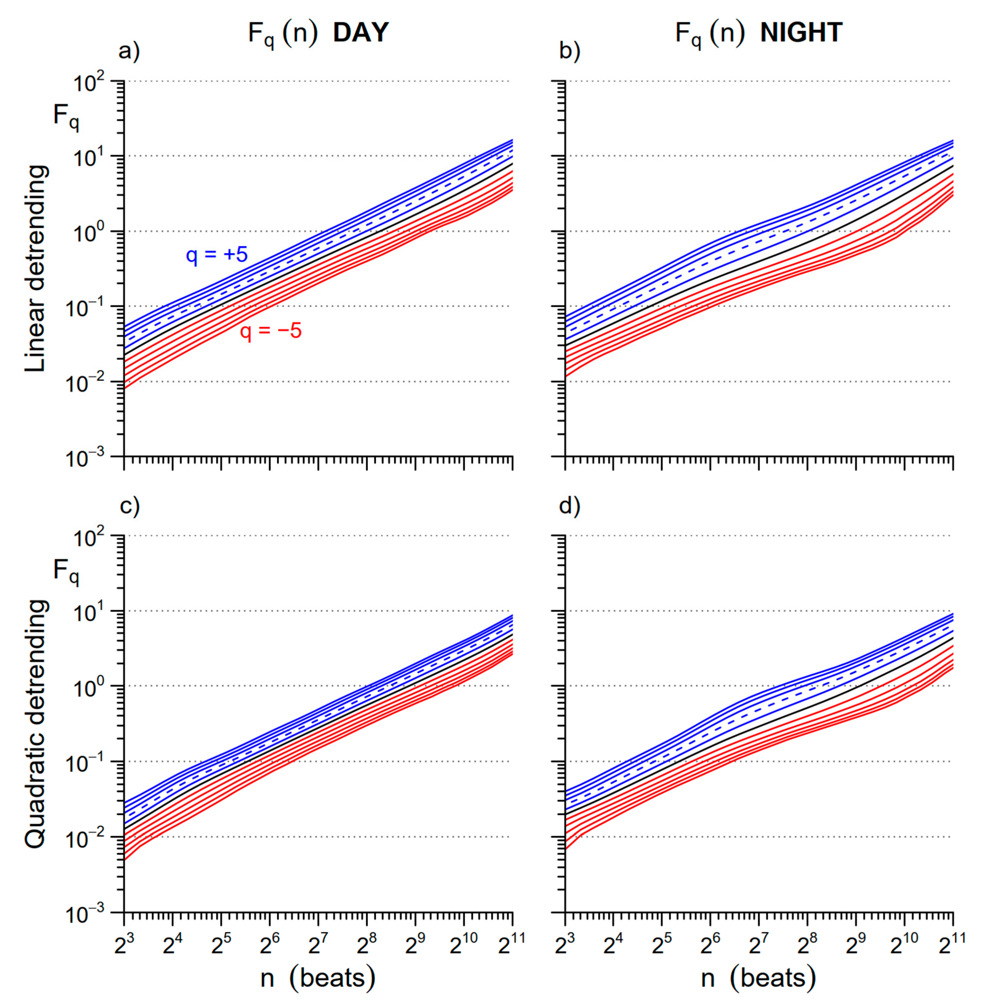
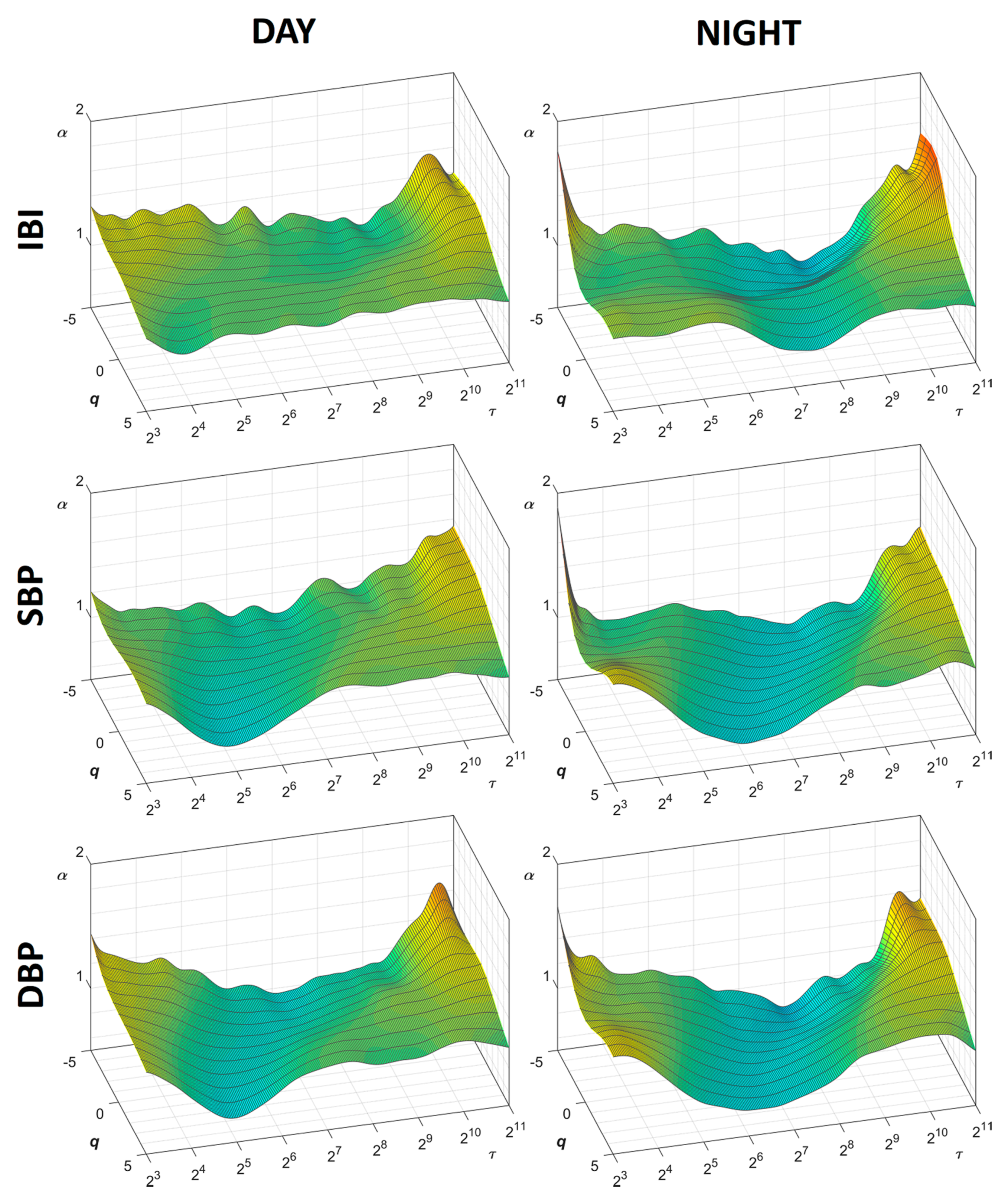
2.2. Multifractal-Multiscale Detrended Fluctuation Analysis
2.3. Nonlinearity Index
2.4. Spectral Analysis
2.5. Statistical Analysis
3. Results
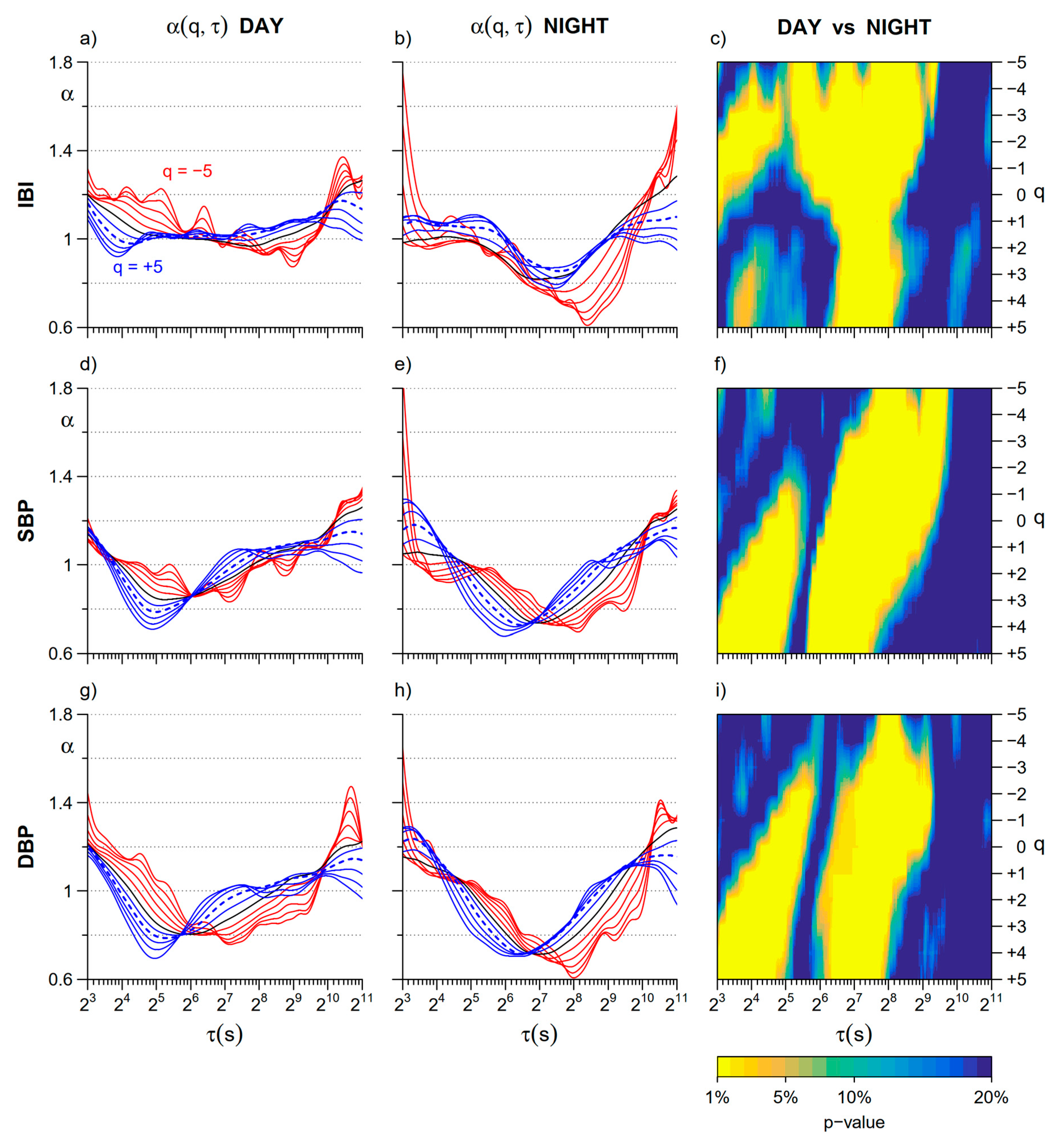
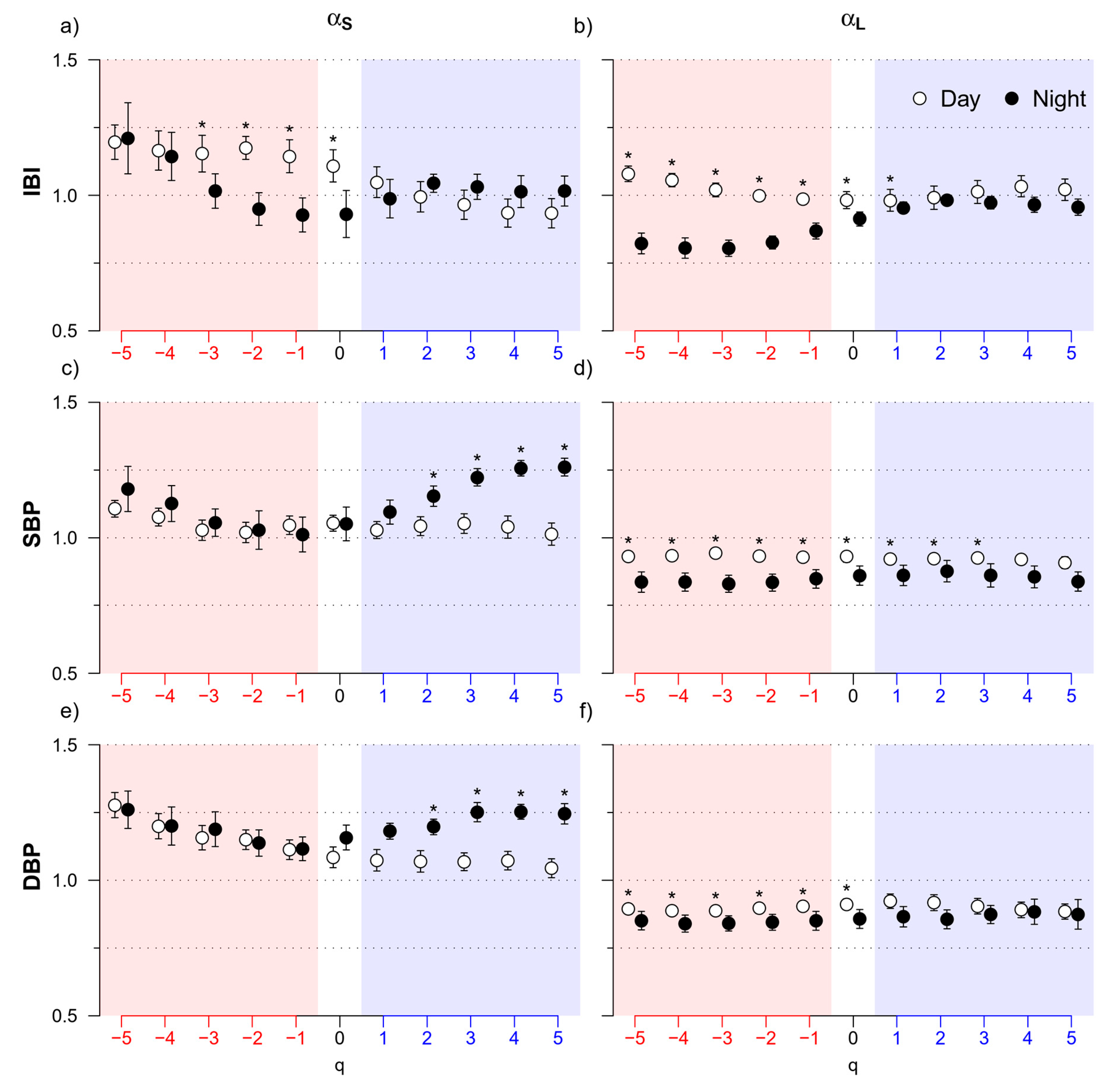
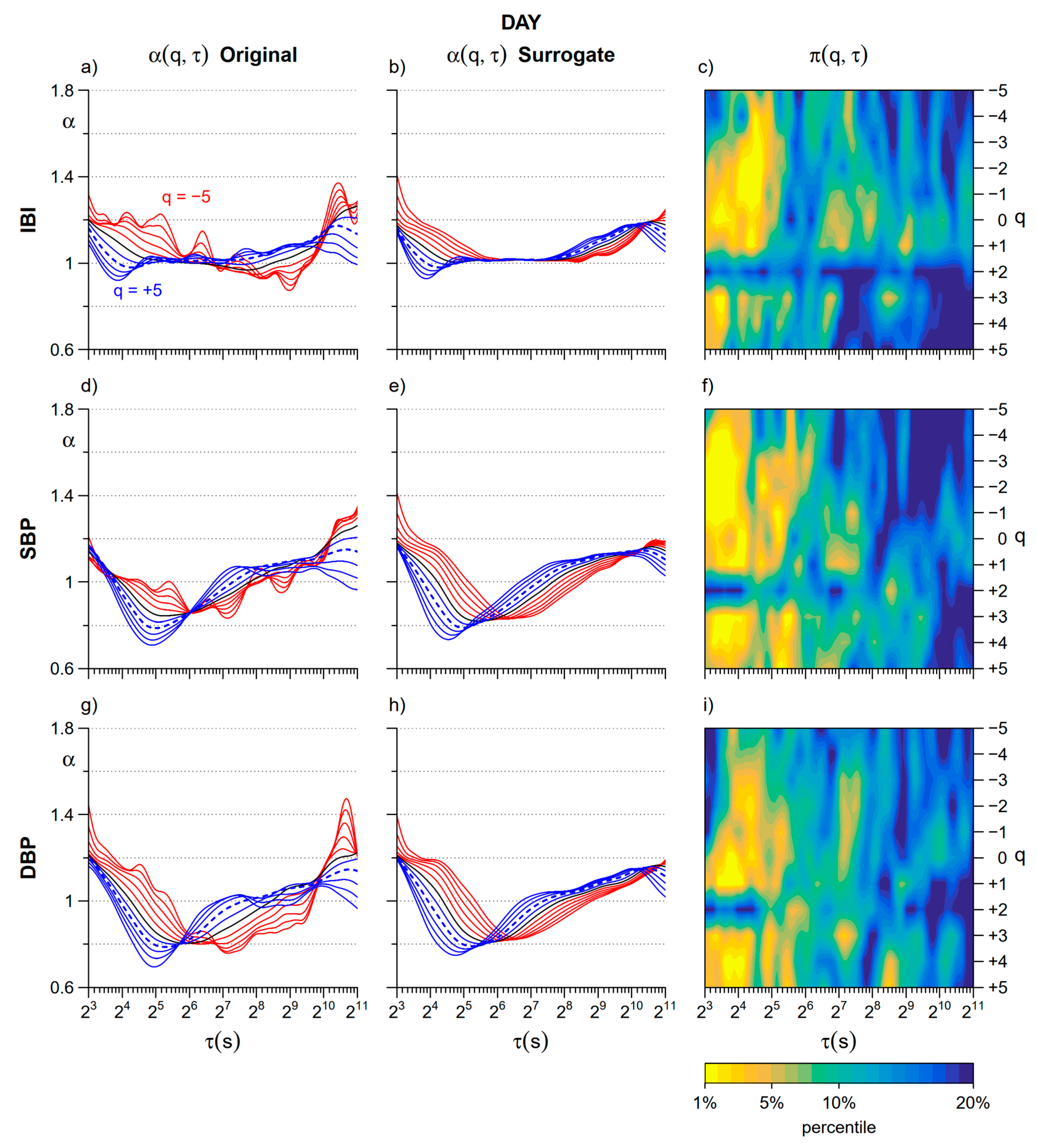
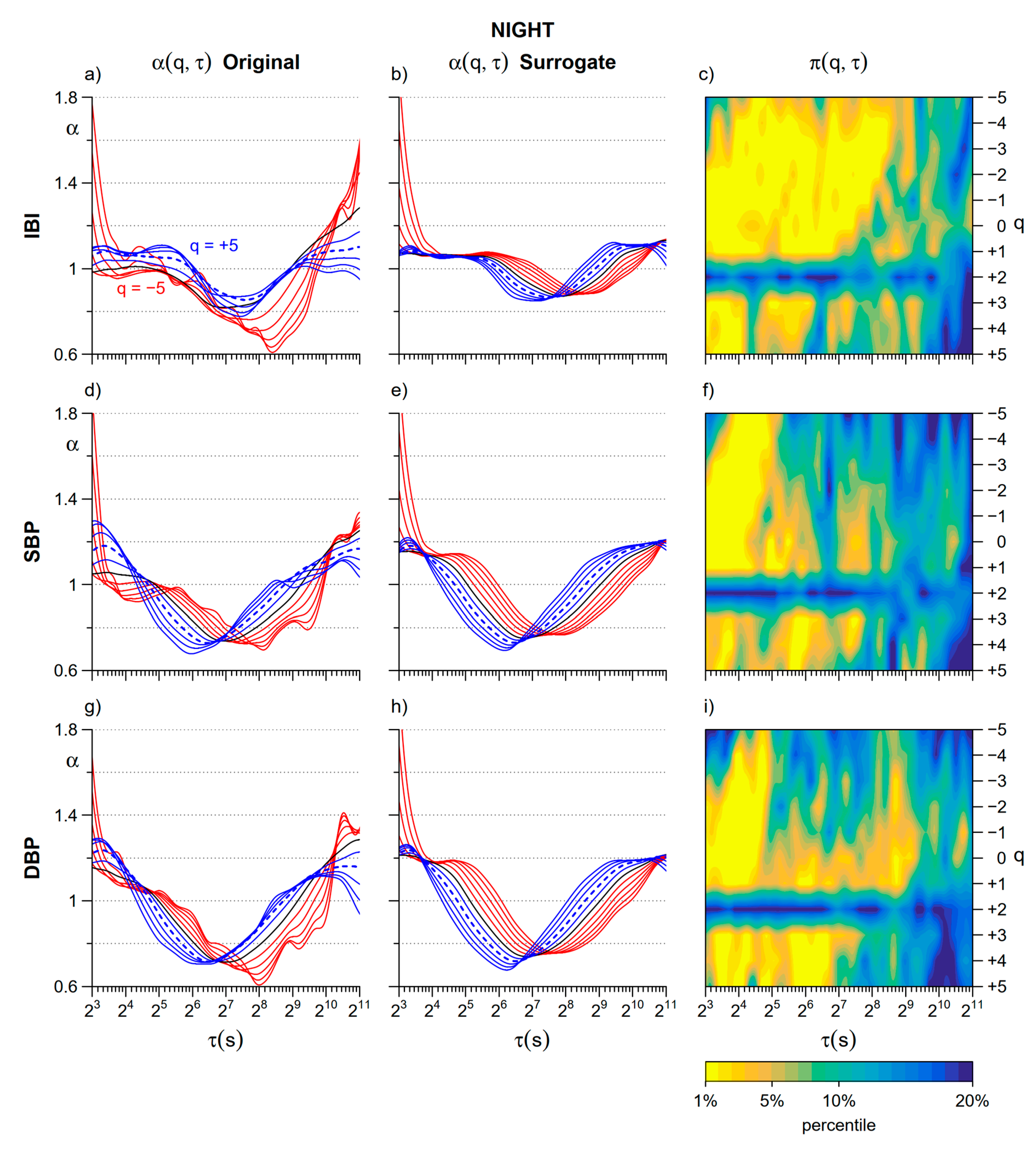
3.1. Day vs. Night
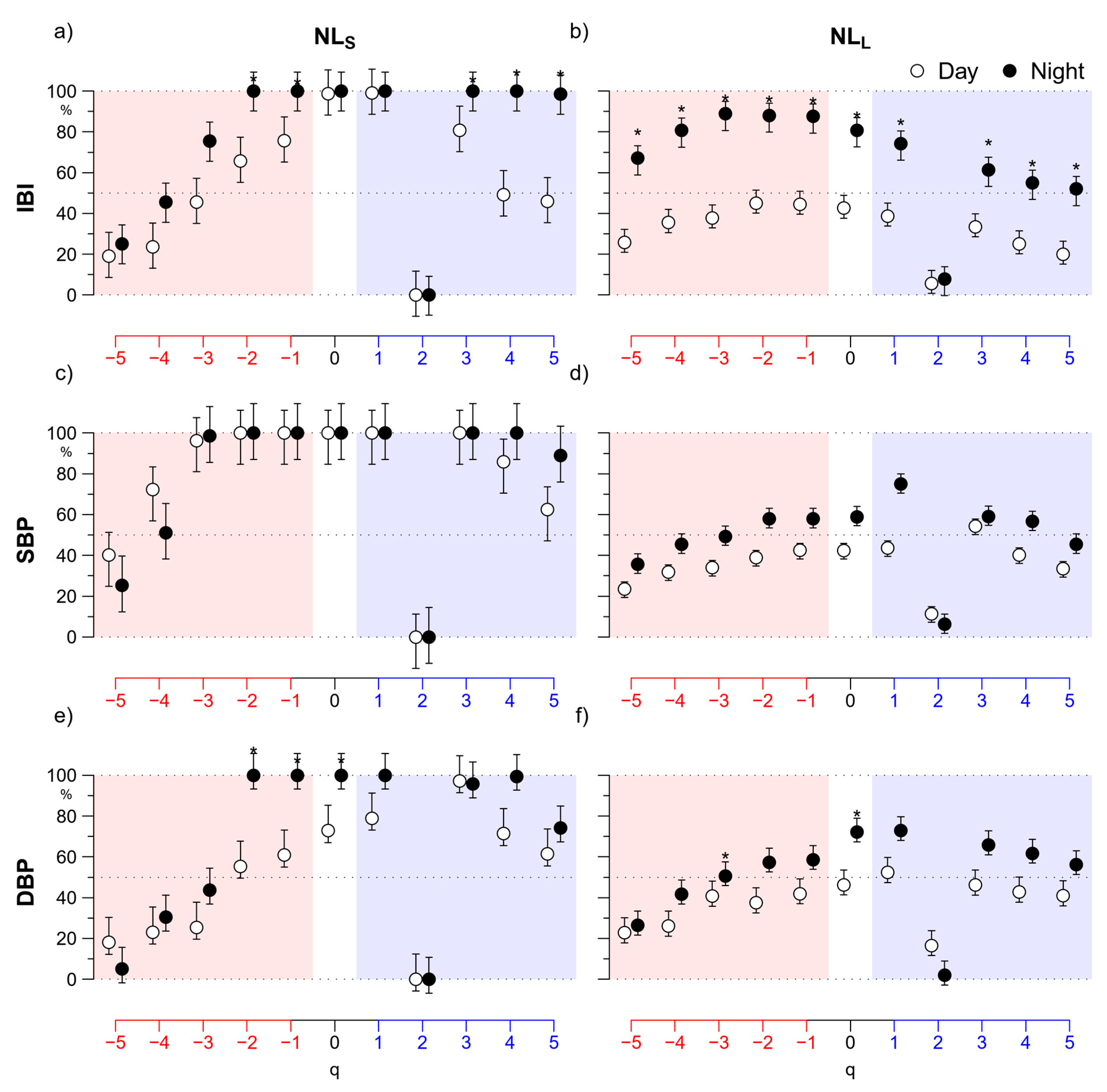
3.2. Nonlinearity
4. Discussion
4.1. Day vs. Night
4.2. Nonlinearity
5. Limitations and Conclusions
Author Contributions
Funding
Conflicts of Interest
References
- Bak, P.; Tang, C.; Wiesenfeld, K. Self-organized criticality: An explanation of the 1/f noise. Phys. Rev. Lett. 1987, 59, 381–384. [Google Scholar] [CrossRef] [PubMed]
- Nagy, Z.; Mukli, P.; Herman, P.; Eke, A. Decomposing Multifractal Crossovers. Front. Physiol. 2017, 8, 8. [Google Scholar] [CrossRef] [PubMed] [Green Version]
- Peng, C.K.; Havlin, S.; Hausdorff, J.M.; E Mietus, J.; Stanley, H.; Goldberger, A.L. Fractal mechanisms and heart rate dynamics. Long-range correlations and their breakdown with disease. J. Electrocardiol. 1995, 28. [Google Scholar] [CrossRef]
- Echeverria, J.C.; Woolfson, M.S.; Crowe, J.A.; Hayes-Gill, B.R.; Croaker, G.D.H.; Vyas, H. Interpretation of heart rate variability via detrended fluctuation analysis and alpha-beta filter. Chaos 2003, 13, 467–475. [Google Scholar] [CrossRef]
- Castiglioni, P.; Parati, G.; Civijian, A.; Quintin, L.; Di Rienzo, M. Local Scale Exponents of Blood Pressure and Heart Rate Variability by Detrended Fluctuation Analysis: Effects of Posture, Exercise, and Aging. IEEE Trans. Biomed. Eng. 2008, 56, 675–684. [Google Scholar] [CrossRef]
- Castiglioni, P.; Parati, G.; Di Rienzo, M.; Carabalona, R.; Cividjian, A.; Quintin, L. Scale exponents of blood pressure and heart rate during autonomic blockade as assessed by detrended fluctuation analysis. J. Physiol. 2010, 589, 355–369. [Google Scholar] [CrossRef]
- Kantelhardt, J.W.; Zschiegner, S.A.; Koscielny-Bunde, E.; Havlin, S.; Bunde, A.; Stanley, H. Multifractal detrended fluctuation analysis of nonstationary time series. Phys. A Stat. Mech. its Appl. 2002, 316, 87–114. [Google Scholar] [CrossRef] [Green Version]
- Makowiec, D.; Rynkiewicz, A.; Wdowczyk-Szulc, J.; Żarczyńska-Buchowiecka, M.; Gała̧ska, R.; Kryszewski, S. Aging in autonomic control by multifractal studies of cardiac interbeat intervals in the VLF band. Physiol. Meas. 2011, 32, 1681–1699. [Google Scholar] [CrossRef]
- Gierałtowski, J.; Żebrowski, J.; Baranowski, R. Multiscale multifractal analysis of heart rate variability recordings with a large number of occurrences of arrhythmia. Phys. Rev. E 2012, 85, 021915. [Google Scholar] [CrossRef]
- Kokosińska, D.; Gierałtowski, J.; Zebrowski, J.J.; Orłowska-Baranowska, E.; Baranowski, R. Heart rate variability, multifractal multiscale patterns and their assessment criteria. Physiol. Meas. 2018, 39, 114010. [Google Scholar] [CrossRef]
- Castiglioni, P.; Merati, G.; Parati, G.; Faini, A. Decomposing the complexity of heart-rate variability by the multifractal-multiscale approach to detrended fluctuation analysis: An application to low-level spinal cord injury. Physiol. Meas. 2019, 40, 084003. [Google Scholar] [CrossRef] [PubMed]
- Heneghan, C.; McDarby, G. Establishing the relation between detrended fluctuation analysis and power spectral density analysis for stochastic processes. Phys. Rev. E 2000, 62, 6103–6110. [Google Scholar] [CrossRef] [PubMed] [Green Version]
- Willson, K.; Francis, D.P. A direct analytical demonstration of the essential equivalence of detrended fluctuation analysis and spectral analysis of RR interval variability. Physiol. Meas. 2002, 24, N1–N7. [Google Scholar] [CrossRef] [PubMed]
- Mancia, G.; Ferrari, A.; Gregorini, L.; Parati, G.; Pomidossi, G.A.; Bertinieri, G.; Grassi, G.; Di Rienzo, M.; Pedotti, A.; Zanchetti, A. Blood pressure and heart rate variabilities in normotensive and hypertensive human beings. Circ. Res. 1983, 53, 96–104. [Google Scholar] [CrossRef] [Green Version]
- Di Rienzo, M.; Castiglioni, P.; Parati, G. Arterial Blood Pressure Processing. In Wiley Encyclopedia of Biomedical Engineering; John Wiley & Sons, Inc.: Hoboken, NJ, USA, 2006; pp. 98–109. [Google Scholar]
- Task Force of the European Society of Cardiology the North American Society of Pacing Electrophysiology. Heart Rate Variability. Circulation 1996, 93, 1043–1065. [Google Scholar] [CrossRef] [Green Version]
- Castiglioni, P.; Faini, A. A Fast DFA Algorithm for Multifractal Multiscale Analysis of Physiological Time Series. Front. Physiol. 2019, 10, 115. [Google Scholar] [CrossRef] [Green Version]
- Kantelhardt, J.W.; Koscielny-Bunde, E.; Rego, H.H.; Havlin, S.; Bunde, A. Detecting long-range correlations with detrended fluctuation analysis. Phys. A Stat. Mech. Appl. 2001, 295, 441–454. [Google Scholar] [CrossRef] [Green Version]
- Bunde, A.; Havlin, S.; Kantelhardt, J.W.; Penzel, T.; Peter, J.-H.; Voigt, K. Correlated and Uncorrelated Regions in Heart-Rate Fluctuations during Sleep. Phys. Rev. Lett. 2000, 85, 3736–3739. [Google Scholar] [CrossRef] [Green Version]
- Castiglioni, P.; Parati, G.; Lombardi, C.; Quintin, L.; Di Rienzo, M. Assessing the fractal structure of heart rate by the temporal spectrum of scale exponents: A new approach for detrended fluctuation analysis of heart rate variability. Biomed. Tech. Eng. 2011, 56, 175–183. [Google Scholar] [CrossRef]
- Gautama, T. Surrogate Data; MATLAB Central File Exchange; MATLAB: Natick, MA, USA, 2005. [Google Scholar]
- Schreiber, T.; Schmitz, A. Surrogate time series. Phys. D Nonlinear Phenom. 2000, 142, 346–382. [Google Scholar] [CrossRef] [Green Version]
- Castiglioni, P.; Parati, G.; Faini, A. Can the Detrended Fluctuation Analysis Reveal Nonlinear Components of Heart Rate Variabilityƒ. In Proceedings of the 2019 41st Annual International Conference of the IEEE Engineering in Medicine and Biology Society (EMBC), Berlin, Germany, 23–27 July 2019; IEEE: Berlin, Germany, 2019; Volume 2019, pp. 6351–6354. [Google Scholar]
- Castiglioni, P.; Parati, G.; Omboni, S.; Mancia, G.; Imholz, B.P.; Wesseling, K.H.; Di Rienzo, M. Broad-band spectral analysis of 24 h continuous finger blood pressure: Comparison with intra-arterial recordings. Clin. Sci. 1999, 97, 129–139. [Google Scholar] [PubMed]
- Di Rienzo, M.; Castiglioni, P.; Mancia, G.; Parati, G.; Pedotti, A. 24 h sequential spectral analysis of arterial blood pressure and pulse interval in free-moving subjects. IEEE Trans. Biomed. Eng. 1989, 36, 1066–1075. [Google Scholar] [CrossRef] [PubMed]
- Parati, G.; Castiglioni, P.; Di Rienzo, M.; Omboni, S.; Pedotti, A.; Mancia, G. Sequential spectral analysis of 24-hour blood pressure and pulse interval in humans. Hypertension 1990, 16, 414–421. [Google Scholar] [CrossRef] [PubMed] [Green Version]
- Castiglioni, P.; Di Rienzo, M.; Veicsteinas, A.; Parati, G.; Merati, G. Mechanisms of blood pressure and heart rate variability: An insight from low-level paraplegia. Am. J. Physiol. Integr. Comp. Physiol. 2007, 292, R1502–R1509. [Google Scholar] [CrossRef] [PubMed] [Green Version]
- Japundžić, N.; Grichois, M.-L.; Zitoun, P.; Laude, D.; Elghozi, J.-L. Spectral analysis of blood pressure and heart rate in conscious rats: Effects of autonomic blockers. J. Auton. Nerv. Syst. 1990, 30, 91–100. [Google Scholar] [CrossRef]
- Hu, K.; Ivanov, P.C.; Hilton, M.F.; Chen, Z.; Ayers, R.T.; Stanley, H.E.; Shea, S. Endogenous circadian rhythm in an index of cardiac vulnerability independent of changes in behavior. Proc. Natl. Acad. Sci. USA 2004, 101, 18223–18227. [Google Scholar] [CrossRef] [Green Version]
- Vandeput, S.; Verheyden, B.; Aubert, A.; Van Huffel, S. Nonlinear heart rate dynamics: Circadian profile and influence of age and gender. Med. Eng. Phys. 2012, 34, 108–117. [Google Scholar] [CrossRef]
- Sassi, R.; Cerutti, S.; Lombardi, F.; Malik, M.; Huikuri, H.V.; Peng, C.-K.; Schmidt, G.; Yamamoto, Y.; Gorenek, B.; Lip, G.Y.; et al. Advances in heart rate variability signal analysis: Joint position statement by the e-Cardiology ESC Working Group and the European Heart Rhythm Association co-endorsed by the Asia Pacific Heart Rhythm Society. Europace 2015, 17, 1341–1353. [Google Scholar] [CrossRef]
- Schmidt, T.F.H.; Wittenhaus, J.; Steinmetz, T.F.; Piccolo, P.; Lüpsen, H. Twenty-Four-Hour Ambulatory Noninvasive Continuous Finger Blood Pressure Measurement with PORTAPRES. J. Cardiovasc. Pharmacol. 1992, 19, S117. [Google Scholar] [CrossRef]
- Constant, I.; Laude, D.; Murat, I.; Elghozi, J.L. Pulse rate variability is not a surrogate for heart rate variability. Clin. Sci. 1999, 97, 391–397. [Google Scholar] [CrossRef] [Green Version]
- Baselli, G.; Cerutti, S.; Civardi, S.; Liberati, D.; Lombardi, F.; Malliani, A.; Pagani, M. Spectral and cross-spectral analysis of heart rate and arterial blood pressure variability signals. Comput. Biomed. Res. 1986, 19, 520–534. [Google Scholar] [CrossRef]


| Day | Night | p Value | |
|---|---|---|---|
| IBI | |||
| mean (ms) | 774.4 (97.3) | 1033.7 (174.1) | <0.01 |
| total power (ms2) | 11,217 (10,569) | 11,751 (7313) | 0.57 |
| VLF power (ms2) | 5885 (5763) | 5905 (3599) | 0.62 |
| LF power (ms2) | 1453 (1219) | 2083 (1946) | 0.25 |
| HF power (ms2) | 538 (576) | 1219 (1036) | <0.01 |
| LF/HF powers ratio | 3.56 (1.4) | 2.21 (1.5) | <0.01 |
| SBP | |||
| mean (mmHg) | 123.7 (12.8) | 108.6 (17.5) | <0.01 |
| total power (mmHg2) | 134.7 (98) | 58.4 (35.4) | <0.01 |
| VLF power (mmHg2) | 65.0 (49.9) | 29.3 (19.4) | <0.01 |
| LF power (mmHg2) | 22.8 (13.4) | 9.7 (6.2) | <0.01 |
| HF power (mmHg2) | 7.3 (4) | 4.0 (2.3) | <0.01 |
| DBP | |||
| mean (mmHg) | 70.2 (8.9) | 60.2 (10.1) | <0.01 |
| total power (mmHg2) | 53.5 (22.6) | 30.4 (17.9) | <0.01 |
| VLF power (mmHg2) | 25.8 (12.7) | 15.3 (9.5) | <0.01 |
| LF power (mmHg2) | 10.3 (4) | 5.6 (3.5) | <0.01 |
| HF power (mmHg2) | 2.8 (1.1) | 1.8 (1.1) | <0.01 |
© 2020 by the authors. Licensee MDPI, Basel, Switzerland. This article is an open access article distributed under the terms and conditions of the Creative Commons Attribution (CC BY) license (http://creativecommons.org/licenses/by/4.0/).
Share and Cite
Castiglioni, P.; Omboni, S.; Parati, G.; Faini, A. Day and Night Changes of Cardiovascular Complexity: A Multi-Fractal Multi-Scale Analysis. Entropy 2020, 22, 462. https://doi.org/10.3390/e22040462
Castiglioni P, Omboni S, Parati G, Faini A. Day and Night Changes of Cardiovascular Complexity: A Multi-Fractal Multi-Scale Analysis. Entropy. 2020; 22(4):462. https://doi.org/10.3390/e22040462
Chicago/Turabian StyleCastiglioni, Paolo, Stefano Omboni, Gianfranco Parati, and Andrea Faini. 2020. "Day and Night Changes of Cardiovascular Complexity: A Multi-Fractal Multi-Scale Analysis" Entropy 22, no. 4: 462. https://doi.org/10.3390/e22040462