Statistical Approaches for the Analysis of Dependency Among Neurons Under Noise


Abstract
:1. Introduction
2. Materials and Methods
2.1. The Hodgkin–Huxley Model
2.2. Information Theory Quantities
2.3. Copulas
2.3.1. Gaussian Copula
2.3.2. Archimedean Copulas
2.4. The Proposed Model and Statistical Analysis
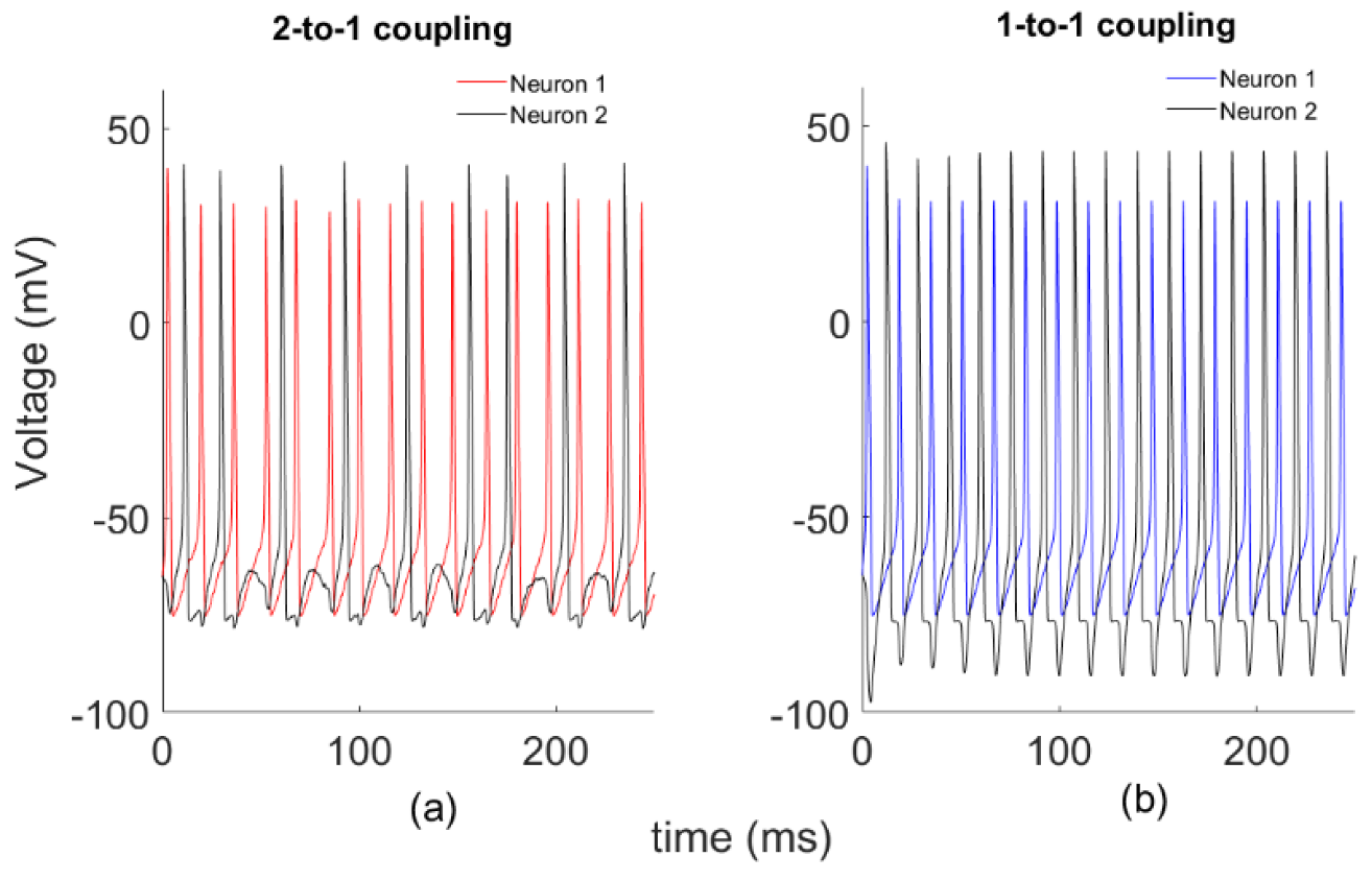
2.4.1. Modeling
2.4.2. Dependency Analysis by MI
2.4.3. Dependency Analysis by Copulas
2.4.4. Directional Dependency Analysis by TE
3. Results
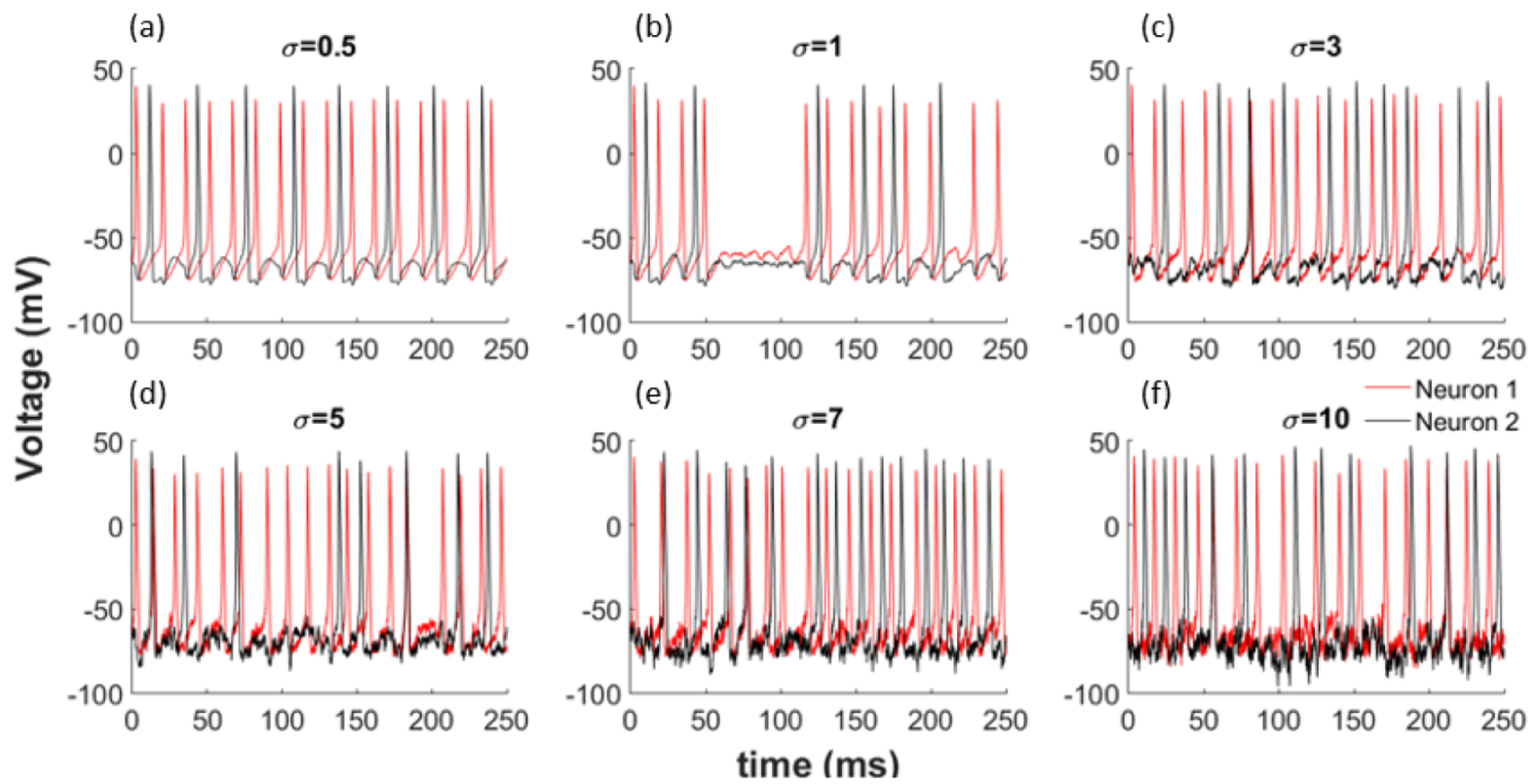
3.1. Data
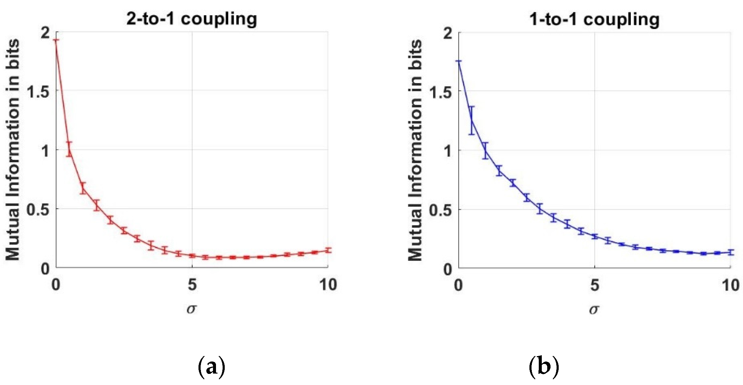
3.2. Dependency Analysis by MI
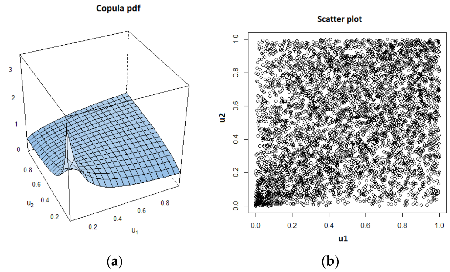
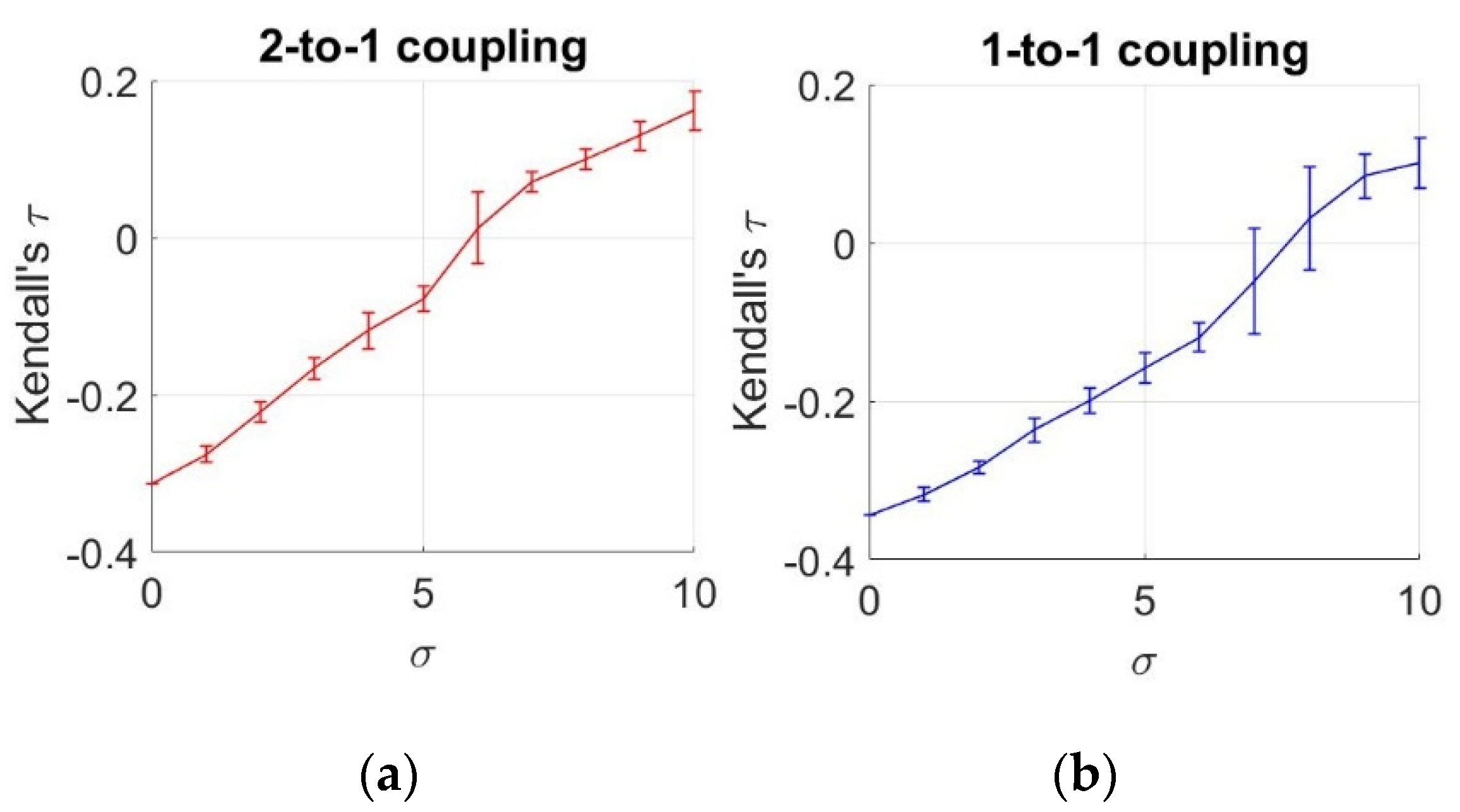
3.3. Dependency Analysis by Copulas
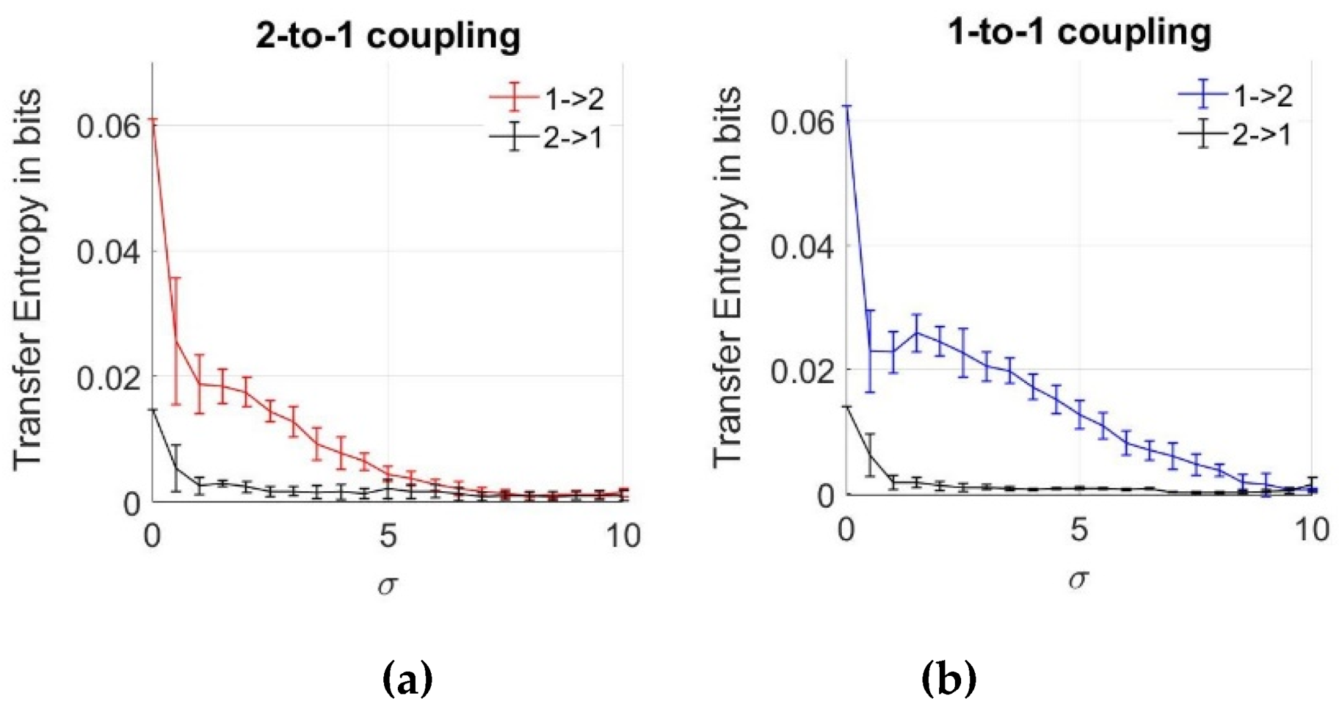
3.4. Dependency Analysis by TE
4. Discussion and Conclusions
Supplementary Materials
Author Contributions
Funding
Conflicts of Interest
Appendix A. Hodgkin–Huxley Model

| Transition rates (ms−1) | ||
| Parameter Values | 1 μF | |
| 8 mA | ||
| 120 μS | ||
| 36 μS | ||
| 0.3 μS | ||
| 50 mV | ||
| −77 mV | ||
| −54.4 mV |
References
- Hodgkin, A.L.; Huxley, A.F. A quantitative description of membrane current and its application to conduction and excitation in nerve. J. Physiol. 1952, 117, 500–544. [Google Scholar] [CrossRef]
- Pandit, S.V.; Clark, R.B.; Giles, W.R.; Demir, S.S. A Mathematical Model of Action Potential Heterogeneity in Adult Rat Left Ventricular Myocytes. Biophys. J. 2001, 81, 3029–3051. [Google Scholar] [CrossRef] [Green Version]
- Bertram, R.; Sherman, A. A calcium-based phantom bursting model for pancreatic islets. Bull. Math. Biol. 2004, 66, 1313–1344. [Google Scholar] [CrossRef] [PubMed]
- Duncan, P.J.; Şengül, S.; Tabak, J.; Ruth, P.; Bertram, R.; Shipston, M.J. Large conductance Ca2+-activated K+ (BK) channels promote secretagogue-induced transition from spiking to bursting in murine anterior pituitary corticotrophs. J. Physiol. 2015, 593, 1197–1211. [Google Scholar] [CrossRef] [PubMed] [Green Version]
- Destexhe, A. Neuronal Noise; Springer: New York, NY, USA, 2012. [Google Scholar]
- Goldwyn, J.H.; Shea-Brown, E. The what and where of adding channel noise to the Hodgkin-Huxley equations. PLoS Comput. Biol. 2011, 7, e1002247. [Google Scholar] [CrossRef] [Green Version]
- Goldwyn, J.H.; Imennov, N.S.; Famulare, M.; Shea-Brown, E. Stochastic differential equation models for ion channel noise in Hodgkin-Huxley neurons. Phys. Rev. E 2011, 83. [Google Scholar] [CrossRef] [PubMed] [Green Version]
- Horikawa, Y. Noise effects on spike propagation in the stochastic Hodgkin-Huxley models. Biol. Cybern. 1991, 66, 19–25. [Google Scholar] [CrossRef]
- Moss, F.; Ward, L.M.; Sannita, W.G. Stochastic resonance and sensory information processing: A tutorial and review of application. Clin. Neurophysiol. 2004, 115, 267–281. [Google Scholar] [CrossRef]
- White, J.A.; Rubinstein, J.T.; Kay, A.R. Channel noise in neurons. Trends Neurosci. 2000, 23, 131–137. [Google Scholar] [CrossRef]
- Ermentrout, G.B.; Galán, R.F.; Urban, N.N. Reliability, synchrony and noise. Trends Neurosci. 2008, 31, 428–434. [Google Scholar] [CrossRef] [Green Version]
- Faisal, A.A.; Selen, L.P.; Wolpert, D.M. Noise in the nervous system. Nat. Rev. Neurosci. 2008, 9, 292–303. [Google Scholar] [CrossRef] [PubMed]
- Lee, K.-E.; Lopes, M.A.; Mendes, J.F.F.; Goltsev, A.V. Critical phenomena and noise-induced phase transitions in neuronal networks. Phys. Rev. E 2014, 89, 012701. [Google Scholar] [CrossRef] [PubMed] [Green Version]
- Lindner, B. Effects of noise in excitable systems. Phys. Rep. 2004, 392, 321–424. [Google Scholar] [CrossRef]
- Brown, E.N.; Kass, R.E.; Mitra, P. PMultiple neural spike train data analysis: State-of-the-art and future challenges. Nat. Neurosci. 2004, 7, 456–461. [Google Scholar] [CrossRef] [PubMed]
- Cohen, M.R.; Kohn, A. Measuring and interpreting neuronal correlations. Nat. Neurosci. 2011, 14, 811–819. [Google Scholar] [CrossRef] [PubMed]
- Yamada, S.; Nakashima, M.; Matsumoto, K.; Shiono, S. Information theoretic analysis of action potential trains. Biol. Cybern. 1993, 68, 215–220. [Google Scholar] [CrossRef]
- Yamada, S.; Matsumoto, K.; Nakashima, M.; Shiono, S. Information theoretic analysis of action potential trains II. Analysis of correlation among n neurons to deduce connection structure. J. Neurosci. Methods 1996, 66, 35–45. [Google Scholar] [CrossRef]
- Wibral, M.; Vicente, R.; Lizier, J.T. Directed Information Measures in Neuroscience; Springer: Basingstoke, UK, 2014. [Google Scholar]
- Li, Z.; Li, X. Estimating Temporal Causal Interaction between Spike Trains with Permutation and Transfer Entropy. PLoS ONE 2013, 8, e70894. [Google Scholar] [CrossRef] [Green Version]
- Ito, S.; Hansen, M.E.; Heiland, R.; Lumsdaine, A.; Litke, A.M.; Beggs, J.M. Extending Transfer Entropy Improves Identification of Effective Connectivity in a Spiking Cortical Network Model. PLoS ONE 2011, 6, e27431. [Google Scholar] [CrossRef]
- Walker, B.L.; Newhall, K.A. Inferring information flow in spike-train data sets using a trial-shuffle method. PLoS ONE 2018, 13, e0206977. [Google Scholar] [CrossRef]
- Nelsen, R.B. An Introduction to Copulas; Springer: New York, NY, USA, 2006. [Google Scholar]
- Belgorodski, N. Selecting Pair-Copula Families for Regular Vines with Application to the Multivariate Analysis of European Stock Market Indices. Diplomarbeit, Technische Universität München, München, Germany, 2010. [Google Scholar]
- Clarke, K.A. A Simple Distribution-Free Test for Nonnested Model Selection. Political Anal. 2007, 15, 347–363. [Google Scholar] [CrossRef]
- Vuong, Q.H. Ratio tests for model selection and non-nested hypotheses. Econometrica 1989, 57, 307–333. [Google Scholar] [CrossRef] [Green Version]
- Schreiber, T. Measuring information transfer. Phys. Rev. Lett. 2000, 85, 461–464. [Google Scholar] [CrossRef] [PubMed] [Green Version]
- Gencaga, D. (Ed.) Transfer Entropy (Entropy Special Issue Reprint); MDPI: Basel, Switzerland, 2018. [Google Scholar]
- Gencaga, D.; Knuth, K.H.; Rossow, W.B. A Recipe for the Estimation of Information Flow in a Dynamical System. Entropy 2015, 17, 438–470. [Google Scholar] [CrossRef] [Green Version]
- Knuth, K.H. Optimal data-based binning for histograms. arXiv 2006, arXiv:physics/0605197. [Google Scholar]
- Scott, D.W. Multivariate Density Estimation: Theory, Practice, and Visualization, 2nd ed.; John Wiley & Sons, Inc.: Hoboken, NJ, USA, 2015. [Google Scholar]
- Darbellay, G.A.; Vajda, I. Estimation of the information by an adaptive partitioning of the observation space. IEEE Trans. Inf. Theory 1999, 45, 1315–1321. [Google Scholar] [CrossRef] [Green Version]
- Timme, N.M.; Lapish, C.C. A tutorial for information theory in neuroscience. eNeuro 2018, 5. [Google Scholar] [CrossRef]
- Brechmann, E.C.; Schepsmeier, U. Modeling Dependence with C- and D-Vine Copulas: The R Package CDVine. J. Stat. Softw. 2013, 52, 1–27. [Google Scholar] [CrossRef] [Green Version]
- Dhanya, E.; Sunitha, R.; Pradhan, N.; Sreedevi, A. Modelling and Implementation of Two Coupled Hodgkin-Huxley Neuron Model. In Proceedings of the 2015 International Conference on Computing and Network Communications, Trivandrum, Kerala, India, 16–19 December 2015. [Google Scholar]
- Ao, X.; Hanggi, P.; Schmid, G. In-phase and anti-phase synchronization in noisy Hodgkin–Huxley neurons. Math. Biosci. 2013, 245, 49–55. [Google Scholar] [CrossRef] [Green Version]
- Cramer, H. Mathematical Methods in Statistics; Princeton University Press: Princeton, NJ, USA, 1946. [Google Scholar]
- Rudolph, M.; Destexhe, A. Correlation Detection and Resonance in Neural Systems with Distributed Noise Sources. Phys. Rev. Lett. 2001, 86, 3662–3665. [Google Scholar] [CrossRef] [Green Version]
- Paninski, L. Estimation of entropy and mutual information. Neural Comput. 2003, 15, 1191–1253. [Google Scholar] [CrossRef] [Green Version]
- Verdú, S. Empirical Estimation of Information Measures: A Literature Guide. Entropy 2019, 21, 720. [Google Scholar] [CrossRef] [Green Version]
- Ermentrout, G. Simulating, Analyzing, and Animating Dynamical Systems; SIAM: Philadelphia, PA, USA, 2002. [Google Scholar]
- Şengül, S.; Clewley, R.; Bertram, R.; Tabak, J. Determining the contributions of divisive and subtractive feedback in the Hodgkin-Huxley model. J. Comput. Neurosci. 2014, 37, 403–415. [Google Scholar] [CrossRef] [PubMed]


| Initial values | V1 = V2 = −65; m1 = m2 = 0.05; h1 = h2 = 0.6; n1 = n2 = 0.317 |
| 1-to-1 coupling | k = 0.25 |
| 2-to-1 coupling | k = 0.1 |
© 2020 by the authors. Licensee MDPI, Basel, Switzerland. This article is an open access article distributed under the terms and conditions of the Creative Commons Attribution (CC BY) license (http://creativecommons.org/licenses/by/4.0/).
Share and Cite
Gençağa, D.; Şengül Ayan, S.; Farnoudkia, H.; Okuyucu, S. Statistical Approaches for the Analysis of Dependency Among Neurons Under Noise. Entropy 2020, 22, 387. https://doi.org/10.3390/e22040387
Gençağa D, Şengül Ayan S, Farnoudkia H, Okuyucu S. Statistical Approaches for the Analysis of Dependency Among Neurons Under Noise. Entropy. 2020; 22(4):387. https://doi.org/10.3390/e22040387
Chicago/Turabian StyleGençağa, Deniz, Sevgi Şengül Ayan, Hajar Farnoudkia, and Serdar Okuyucu. 2020. "Statistical Approaches for the Analysis of Dependency Among Neurons Under Noise" Entropy 22, no. 4: 387. https://doi.org/10.3390/e22040387