Article

An Extended FMEA Model Based on Cumulative Prospect Theory and Type-2 Intuitionistic Fuzzy VIKOR for the Railway Train Risk Prioritization

1
State Key Laboratory of Rail Traffic Control and Safety, Beijing Jiaotong University, Beijing 100044, China
2
School of Traffic and Transportation, Beijing Jiaotong University, Beijing 100044, China
3
School of Economics and Management, Southeast University, Nanjing 211189, China
*
Author to whom correspondence should be addressed.
Entropy 2020, 22(12), 1418; https://doi.org/10.3390/e22121418
Submission received: 2 December 2020 / Revised: 11 December 2020 / Accepted: 13 December 2020 / Published: 15 December 2020

Abstract

:
This paper aims toward the improvement of the limitations of traditional failure mode and effect analysis (FMEA) and examines the crucial failure modes and components for railway train operation. In order to overcome the drawbacks of current FMEA, this paper proposes a novel risk prioritization method based on cumulative prospect theory and type-2 intuitionistic fuzzy VIKOR approach. Type-2 intuitionistic VIKOR handles the combination of the risk factors with their entropy weight. Triangular fuzzy number intuitionistic fuzzy numbers (TFNIFNs) applied as type-2 intuitionistic fuzzy numbers (Type-2 IFNs) are adopted to depict the uncertainty in the risk analysis. Then, cumulative prospect theory is employed to deal with the FMEA team member’s risk sensitiveness and decision-making psychological behavior. Finally, a numerical example of the railway train bogie system is selected to illustrate the application and feasibility of the proposed extended FMEA model in this paper, and a comparison study is also performed to validate the practicability and effectiveness of the novel FMEA model. On this basis, this study can provide guidance for the risk prioritization of railway trains and indicate a direction for further research of risk management of rail traffic.

1. Introduction

As a kind of reliability analysis and risk management technique, failure mode and effect analysis (FMEA) has been widely used in rail traffic risk analysis [1,2]. In practice, the risk prioritization of every failure mode can be obtained by a risk priority number (RPN) through three risk factors of occurrence (O), severity (S) and detection (D). Then, the key components can be identified by the fusion of the RPN of each failure mode [3].
Despite the simplicity and understandability of the RPN method for the railway train risk analysis and prioritization, it still possesses many drawbacks. The most criticized drawbacks are presented as follows [4,5,6,7]:
  • The multiplication for the RPN can be questionable and sensitive to the variations in risk factors calculation.
  • Different combination of the risk factor O, S and D can produce the same RPN value, which is not effective in practical risk management.
  • The risk factor O, S and D can be difficult to determined precisely in many real-world scenarios.
  • The relative importance among the risk factor O, S and D can be overlooked in the conventional FMEA approach.
The most important and urgent business is to determine the criticality of the system component in the operation of railway train. Later, the maintenance optimization and improvement can be put into practice for the safety and reliability operation.
As stated above, there is a pressing need to further improve the conventional FMEA approach for the railway train risk analysis and prioritization. In order to overcome the shortcomings of traditional FMEA approach, some applications employed the risk information judgments with linguistic terms of fuzzy set theory. Triangular fuzzy numbers [8,9], interval fuzzy numbers [10], hesitant fuzzy numbers [11,12] and intuitionistic fuzzy numbers (IFNs) [13,14] have been adopted with MCDM methods to deal with the risk prioritization problems. By comparison, IFNs can be characterized by the membership function (MF) and non-membership function (NMF) to illustrate the positive and negative degree, respectively, which can be more flexible than other fuzzy terms. Nevertheless, it can be a challenge to determine the accurate data of their MFs and NMFs. Hence, type-2 IFNs have been put forward to handle the fuzzy problems in a way. Type-2 IFNs possess many advantages over IFNs, as their MFs and NMFs are themselves fuzzy, making it possible to model and minimize the effects of indeterminacy in fuzzy matters. Yu, Wang and Wang [15] extended IFNs with interval numbers as an application of type-2 IFNs for the uncertainty in the site-selection problem. Wei et al. [16] applied interval valued IFNs with entropy measures to overcome the existing entropy matters. However, the terminal point of MFs and NMFs can be difficult to determine and further enlarge the interval area after arithmetic operation. Therefore, Liu and Yuan [17] proposed TFNIFNs as another application of type-2 IFS to describe uncertainty and fuzziness. Compared with interval valued IFNs, TFNIFNs [18] can be better utilized in the fields of fuzziness as the triangular fuzzy number between 0 and 1, which can make TFNIFNs more flexible and reasonable.
On the other hand, some papers regarded the risk prioritization as a multi-criteria decision making (MCDM) problem [19,20,21,22,23,24]. Consequently, the MCDM model has been widely applied to solve the drawbacks in FMEA. Among the different MCDM technologies, TOSPIS and VIKOR methods are the widely used applications. Liu et al. [25] developed FMEA and VIKOR method to identify the risk of general anesthesia process. Lo et al. [26] proposed a novel FMEA model based on TOPSIS method for the equipment product risk identification. Furthermore, Mandal et al. [27] present a FMEA framework with fuzzy VIKOR approach for safety critical resources identification and risk mitigation purposes. Li et al. [28] tried to identify, evaluate and eliminate potential failures of the spindle box system by an advanced FMEA combined with fuzzy TOPSIS. According to the above researches, the solution obtained by the VIKOR method [29] is an aggregation of all the criteria, the relative importance of the criteria, and a balance between total and individual satisfaction. However, the solution determined by TOPSIS method considers the distances from the ideal point and negative-ideal point without considering their relative importance. Therefore, the comparison cases indicate that the VIKOR method can be slightly better than the TOPSIS method [30,31].
Although, to some extent, these efforts have eliminated the shortcomings of the conventional FMEA, there is a crucial issue that has not been fully coped with, namely, experts’ risk sensitiveness and decision-making psychological behavior. In order to solve this problem, prospect theory [32,33,34,35] combined with MCDM methods can be used to conduct risk prioritization in FMEA model by the consideration of experts’ risk sensitiveness and decision-making psychological behavior. However, traditional prospect theory also has the unacceptable drawback about violations of dominance. Consequently, cumulative prospect theory [36] has been proposed to handle this matter. In cumulative prospect theory, the probability weight is replaced by cumulative probability weight and makes it a clear logic as well as a relatively simple computation procedure, thus, cumulative prospect theory can be extensively applied in various MCDM problems [37,38,39,40].
According to the discussion above, in this paper, we develop an extended FMEA model based on cumulative prospect theory and type-2 intuitionistic fuzzy VIKOR for the railway train risk prioritization. In order to handle such situations where experts with different risk sensitiveness and decision-making psychological behavior towards different failure modes of railway train, cumulative prospect theory combined with TFNIFNs is adopted to depict the different risk sensitiveness and psychological behavior of experts. In addition, the VIKOR approach associated with entropy weight method is also carried out to fuse the risk information under different risk factors. Therefore, the final risk prioritization order can be obtained based on the compromise results of VIKOR. At last, a case study of railway train bogie system is utilized to illustrate the proposed extended FMEA model.
In the light of the above analysis, the contributions of this paper can be summarized as follows:
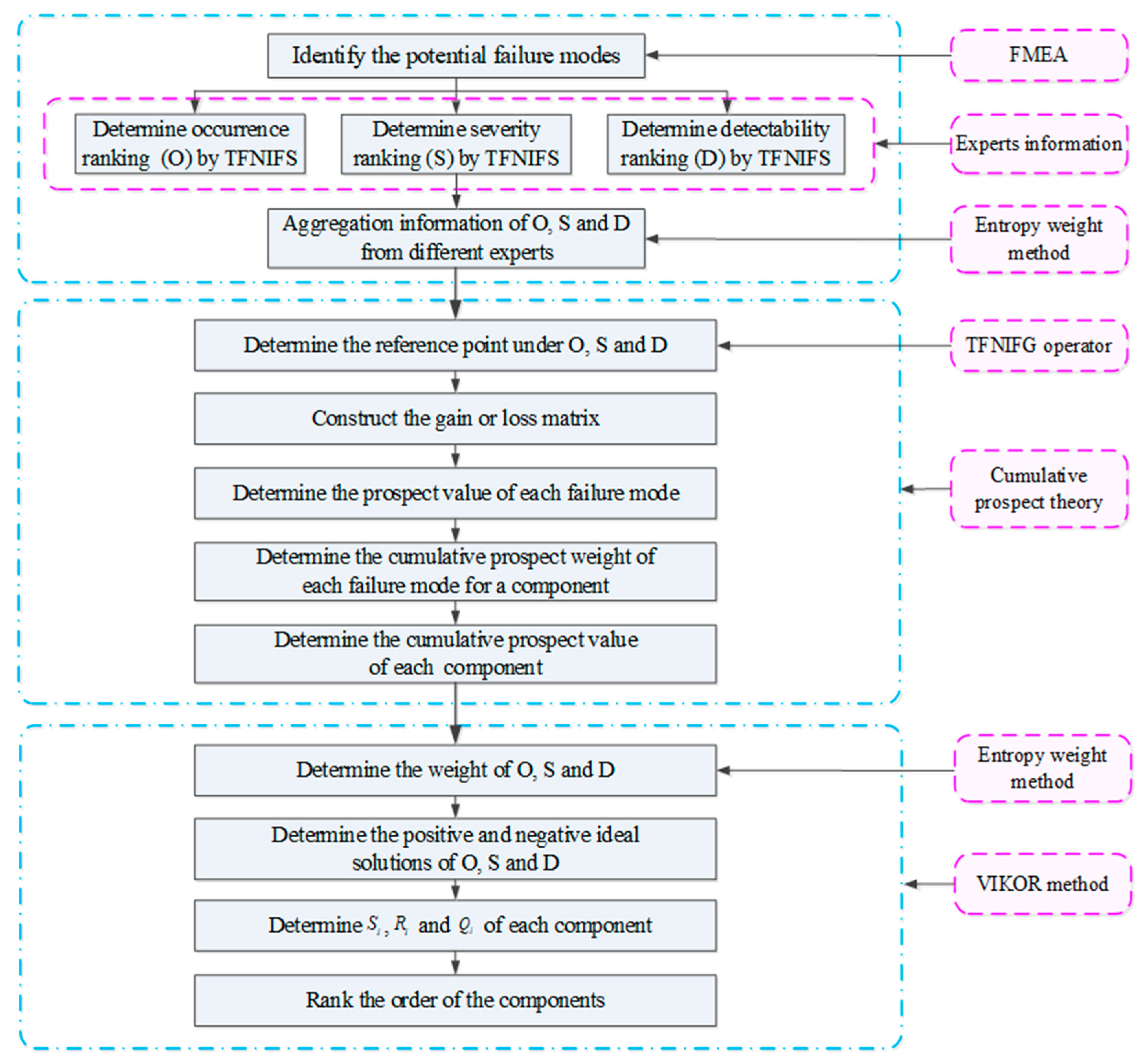
  • The proposed risk component prioritization model based on FMEA framework considers all possible failure modes of railway train without losing any valid state information.
  • The extended FMEA model combined with cumulative prospect theory considers the experts’ risk sensitiveness and decision-making psychological behavior which can obtain a relatively objective and reasonable risk prioritization outcome.
  • The application of triangular fuzzy number intuitionistic fuzzy geometric (TFNIFG) operator as reference point can integrate all the risk score information comprehensively to determine the cumulative prospect value of each failure mode.
The rest of this paper can be organized as follows. In Section 2, the basic theories related to type-2 intuitionistic fuzzy numbers, VIKOR and cumulative prospect theory are briefly introduced. Section 3 presents the extended FMEA model based on cumulative prospect theory and type-2 intuitionistic fuzzy VIKOR for the railway train risk prioritization. In Section 4, a case study of the railway train bogie system is selected to illustrate the application and effectiveness of the proposed method. In Section 5, the conclusions and future research directions of this study are provided.

2. Preliminaries

This paper develops an extended FMEA model based on cumulative prospect theory and type-2 intuitionistic fuzzy VIKOR for the railway train risk prioritization. In this section, the basic concepts of TFNIFNs, VIKOR method and cumulative prospect theory are briefly introduced, which will be utilized in the subsequent sections.

2.1. TFNIFNs

Definition 1
([41]). Let X be a fixed set, an IFN A in X can be defined as
A = { x , u A ( x ) , v A ( x ) | x X }
In which uA(x): X→[0, 1] and vA(x): X→[0, 1] is MF and NMF, respectively, satisfying 0 ≤ uA(x) + vA(x) ≤ 1, x X . The number uA(x) and vA(x) shows the degree of MF and NMF of x to A, for all x X , respectively.
Definition 2
([18]). A triangular fuzzy number C = (l, m, r) in X is a special fuzzy number, its MF can be defined as
u C ( x ) = { ( x l ) / ( m l ) , l x m ( x r ) / ( m r ) , m x r 0 , o t h e r w i s e
In which 0 l m r 1 , m is the barycenter of triangular fuzzy number C, if l = m = r, then C is an accurate number.
As for a triangular fuzzy number C, its fuzzy mean E(C) and standard deviation σ(C) can be defined as
E ( C ) = l + 2 m + r 4
σ ( C ) = 3 l 2 + 4 m 2 + 3 r 2 4 l m 2 l r 4 m r 80
Definition 3
([18]). Let A ˜ = { x , u A ˜ ( x ) , v A ˜ ( x ) | x X } be a TFNIFN, and its MF u A ˜ ( x ) and NMF v A ˜ ( x ) is a triangular fuzzy number, respectively.
Let A ˜ = { x , u A ˜ ( x ) , v A ˜ ( x ) | x X } be a TFNIFN, then the score function and variation function of A ˜ can be defined as
S ( A ˜ ) = E ( μ A ˜ ) 1 + E ( μ A ˜ ) E ( ν A ˜ ) 2 ( 1 E ( μ A ˜ ) E ( ν A ˜ ) )
G ( A ˜ ) = σ ( μ A ˜ ) + σ ( ν A ˜ )
Let A 1 ˜ and A 2 ˜ be two TFNIFNs, we can define that:
If S ( A 1 ˜ ) < S ( A 2 ˜ ) , then A 1 ˜ < A 2 ˜ ;
If S ( A 1 ˜ ) = S ( A 2 ˜ )   a n d   G ( A 1 ˜ ) = G ( A 2 ˜ ) , then A 1 ˜ = A 2 ˜ ;
If S ( A 1 ˜ ) = S ( A 2 ˜ )   a n d   G ( A 1 ˜ ) > G ( A 2 ˜ ) , then A 1 ˜ < A 2 ˜ .
Definition 4
([18]). Let A ˜ i = ( ( a l i , a m i , a r i ) , ( b l i , b m i , b r i ) ) be a set of TFNIFNs, i = 1, 2, …, N. The TFNIFG operator r ˜ can be defined as
r ˜ = ( A ˜ 1 ) 1 / N ( A ˜ 2 ) 1 / N ( A ˜ N ) 1 / N = ( ( i = 1 N ( a l i ) 1 / N , i = 1 N ( a m i ) 1 / N , i = 1 N ( a r i ) 1 / N ) , ( ( 1 i = 1 N ( 1 b l i ) 1 / N ) , ( 1 i = 1 N ( 1 b m i ) 1 / N ) , ( 1 i = 1 N ( 1 b r i ) 1 / N ) ) )
Definition 5
([42]). Let A ˜ 1 = ( ( a l 1 , a m 1 , a r 1 ) , ( b l 1 , b m 1 , b r 1 ) ) and A ˜ 2 = ( ( a l 2 , a m 2 , a r 2 ) , ( b l 2 , b m 2 , b r 2 ) ) be two TFNIFNs. The Hamming distance between A ˜ 1 and A ˜ 2 can be defined as
d ( A ˜ 1 , A ˜ 2 ) = 1 8 ( | a l 1 a l 2 | + 2 | a m 1 a m 2 | + | a r 1 a r 2 | + | b l 1 b l 2 | + 2 | b m 1 b m 2 | + | b r 1 b r 2 | )

2.2. VIKOR Approach

The VIKOR approach proposed by Opricovic in 1998 is a widely used MCDM technique [27]. VIKOR approach is a compromise sorting method that can compromise ranking of a finite decision scheme by maximizing group utility and minimizing individual regret. The key idea of the VIKOR method is to select the optimal solution based on the closeness degree by each evaluation value, positive ideal solution and negative ideal solution. The procedure of VIKOR approach can be given below.
Step 1: Determine the positive ideal solution f j + and negative ideal solution f j from the evaluation matrix.
f j + = max f i j , f j = min f i j
Step 2: Determine the maximizing group utility Si and minimizing individual regret Ri from the evaluation matrix.
S i = j = 1 m w j d ( f j + , f i j ) d ( f j + , f j )
R i = max j   w j d ( f j + , f i j ) d ( f j + , f j )
In which wj is the weight of criteria.
Step 3: Determine the compromise solution Qi.
Q i = ν ( S i S ) ( S S ) + ( 1 ν ) ( R i R ) ( R R )
In which v is the weight of the strategy of “the majority of criteria’’. The value of v lies in the range of 0–1. Normally, the value of v can be considered as 0.5. The intermediate parameters S*, S, R* and R can be given below.
S = min i   S i ,   S = max i   S i ,   R = min i   R i ,   R = max i   R i
Step 4: Determine the prioritization order of alternatives according to ascending order by the compromise solution Qi.

2.3. Cumulative Prospect Theory

Cumulative prospect theory put forward by Tversky and Kahneman in 1992 is an extended method of prospect theory [36]. It is a useful tool for assessment and decision making under risk and uncertainties in consideration of experts’ risk sensitiveness and decision-making psychological behavior. The significant enhancement of cumulative prospect theory compared with prospect theory is that the weight function is an inverse S-type curve. In cumulative prospect theory, the cumulative prospect value V can be determined as
V = i = m 0 v ( Δ x i j ) Π i + i = 1 n v ( Δ x i j ) Π i +
In which v ( Δ x i j ) is the value function and demonstrates the gains or losses of the alternative. It can be determined as:
v ( Δ x i j ) = { ( x i j x j ) α , x i j x j λ ( x i j x j ) β , x i j < x j
where xij is the outcome of the alternative ij, xj is the reference point of the alternative ij under the criterion j. α and β are the exponential parameters related to gains and losses. λ is the risk aversion parameter, and it represents the characteristic of steeper for losses than for gains. Based on the experiment validation [36], these parameters can be provided as α = β = 0.88, λ = 2.25.
Π i and Π i + are the decision weight and can be expressed as follows when the value function v ( Δ x i j ) > 0 and v ( Δ x i j ) < 0 , respectively.
Π i + = w + ( p i + p i + 1 + + p n ) w + ( p i + 1 + p i + 2 + + p n )
Π i = w ( p m + p m + 1 + + p i ) w ( p m + p m + 1 + + p i 1 )
where w+ and w are the weight functions and are strictly increasing functions from the unit interval into itself. The weight function w+ and w can be expressed as
w + ( p ) = p γ [ p γ + ( 1 p ) γ ] 1 γ
w ( p ) = p δ [ p δ + ( 1 p ) δ ] 1 δ
where γ and δ are the attitude parameters for gains and losses. Generally, the values of γ and δ can be provided as 0.61 and 0.69, respectively [36].

3. The Proposed FMEA Model for Railway Train Risk Prioritization

In this section, a comprehensive FMEA model based on cumulative prospect theory and type-2 intuitionistic fuzzy VIKOR is developed to analyze the risk of railway train and rank the crucial components.
The risk prioritization in FMEA model can be treated as a MCDM problem, and the risk factor O, S and D can be regarded as a group of decision criteria. As a result, the procedure of resolving this FMEA problem can be considered as a process of risk prioritization where uncertainty and FMEA team members’ preference and psychological behavior are both taken into account. The general steps for this proposed FMEA model can be illustrated as Figure 1 and the systematic procedures can be briefly introduced as follows.

3.1. Determine and Aggregate the FMEA Decision Value by Type-2 Intuitionistic Fuzzy Number

In the process of failure mode and component risk prioritization, we can assume that there are m alternatives, namely system components denoted by Ai (i = 1, 2, …, m), t failure modes for a component Ai, presented by FMis (is = 1, 2, …, t), 3 criteria, namely risk factor O, S and D, indicated by Cj (j = 1, 2, 3), and l decision makers, namely FMEA team members, expressed by DMk (k = 1, 2, …, l). Let r i s j k be the decision value for the failure mode FMis on criterion Cj about the FMEA team member DMk. Moreover, in light of uncertainty of the risk factor O, S and D, the decision value can be expressed by TFNIFNs presented as r i s j k = ( ( a l i s j k , a m i s j k , a r i s j k ) , ( b l i s j k , b m i s j k , b r i s j k ) ) .
Every FMEA team member is required to give the risk score of the failure mode FMis on criterion Cj by TFNIFNs, as provided in Table 1, Table 2 and Table 3, respectively.
With respect to the different FMEA team members, the different risk score information needs to be aggregated based on the team members’ weight. In the literature [43], there are various approaches to calculate the importance weight of different expert, such as AHP method [44], distance-based method [45], SWARA method [46] and entropy weight method [23,30], etc. The entropy weight method has been widely used in the MCDM problems, and it can illustrate relative information more objectively [23,30]. Therefore, the entropy weight method is applied to determine the weights of FMEA team members in this paper. The process to determine the FMEA team members’ weights can be briefly explained as follows.
Step 1: Determine the TFNIFG operator r ˜ j k of each FMEA team member under different risk factors.
r ˜ j k = ( ( i s = 1 N ( a l i s j k ) 1 / N , i s = 1 N ( a m i s j k ) 1 / N , i s = 1 N ( a r i s j k ) 1 / N ) , ( ( 1 i s = 1 N ( 1 b l i s j k ) 1 / N ) , ( 1 i s = 1 N ( 1 b m i s j k ) 1 / N ) , ( 1 i s = 1 N ( 1 b r i s j k ) 1 / N ) ) )
Step 2: Determine the risk score information entropy of each FMEA team member under different risk factors.
e j k = 1 ln ( N ) i s = 1 N d ( r i s j k , r ˜ j k ) i s = 1 N d ( r i s j k , r ˜ j k ) ln ( d ( r i s j k , r ˜ j k ) i s = 1 N d ( r i s j k , r ˜ j k ) )
Step 3: Determine the importance weight of different FMEA team member under different risk factors.
w j k = 1 e j k k = 1 l 1 e j k
Consequently, the aggregated risk score information of failure mode FMis can be gathered as r i s j = ( ( a l i s j , a m i s j , a r i s j ) , ( b l i s j , b m i s j , b r i s j ) ) .

3.2. Determine the Cumulative Prospect Value of Each Component

In this part, different failure modes of a component can be regarded as the different performance states of the component. As for the component risk, it refers to the different performance states of a component with different probability. As a result, the component risk associated with different failure modes can be determined based on the cumulative prospect theory. The procedure to calculate the cumulative prospect value of each component can be summarized as follows.
Step 1: Determine the reference points under different risk factors.
With respect to the risk score information of different failure mode, it expresses as TFNIFN. Consequently, the reference points can be designed as the TFNIFG operator for a set of risk score information. Let rj = ((alj, amj, arj), (blj, bmj, brj)) be the reference point under risk factor Cj. rj can be expressed as
r ˜ j = ( ( i s = 1 N ( a l i s j ) 1 / N , i s = 1 N ( a m i s j ) 1 / N , i s = 1 N ( a r i s j ) 1 / N ) , ( ( 1 i s = 1 N ( 1 b l i s j ) 1 / N ) , ( 1 i s = 1 N ( 1 b m i s j ) 1 / N ) , ( 1 i s = 1 N ( 1 b r i s j ) 1 / N ) ) )
Step 2: Determine and construct the gain or loss matrix.
After determining the reference point, the gain or loss value of a failure mode can be constructed based on Hamming distance between aggregated risk score information and reference point.
v ( Δ r i s j ) = { d ( r i s j , r j ) 0.88 , r i s j r j 2.25 d ( r i s j , r j ) 0.88 , r i s j < r j
Consequently, the gain or loss matrix of the failure modes can be expressed as follows.
         C 1    C 2    C n V = A 1   F M 11 A 1   F M 12 A m   F M m t [ v ( Δ r 111 ) v ( Δ r 112 ) v ( Δ r 11 n ) v ( Δ r 121 ) v ( Δ r 122 ) v ( Δ r 12 n ) v ( Δ r m t 1 ) v ( Δ r m t 2 ) v ( Δ r m t n ) ]
Step 3: Determine the cumulative prospect weight of each failure mode for a component.
Based on the step 2, the importance weight of each failure mode for a component can be obtained based on the cumulative prospect theory. The cumulative prospect weight is the promotion of the traditional prospect weight as it considers the cumulative probability rather than a single probability. Therefore, the order of gain or loss value of failure modes for a component can be determined by increasing ranking. Let −misn, the ranking order can be denoted as v ( Δ r m ) v ( Δ r m + 1 ) v ( Δ r i s j ) v ( Δ r n 1 ) v ( Δ r n ) . The failure mode FMis and probability pis under the risk factor Cj is associated with v ( Δ r i s j ) . Thus, the cumulative prospect weight of each failure mode can be determined as follows.
Π i s + = w + ( p i s + p i s + 1 + + p n ) w + ( p i s + 1 + p i s + 2 + + p n ) , 0 i s < n Π i s = w ( p m + p m + 1 + + p i s ) w ( p m + p m + 1 + + p i s 1 ) , m < i s 0
In which the weight function w+ and w can be determined in accordance with Equations (18) and (19), Π n + = w + ( p n ) and Π m = w ( p m ) .
Step 4: Determine the cumulative prospect value of each component.
Based on the gain or loss matrix and cumulative prospect weight of the failure modes, the cumulative prospect value of a component can be expressed as follows.
V A i j = i s = m 0 v ( Δ r i s j ) Π i s + i s = 1 n v ( Δ r i s j ) Π i s +

3.3. Determine the Component Risk Prioritization by VIKOR

After determining the cumulative prospect value of each component under different risk factors, the comprehensive risk ranking and prioritization of the system component can be determined based on the VIKOR method. The importance weight of different risk factors can be calculated by entropy weight method [23]. The procedure to determine the comprehensive risk prioritization of each component can be summarized as follows.
Step 1: Determine the importance weight of risk factor O, S and D.
Based on the cumulative prospect value of components, the risk information entropy of different factors can be expressed as follows.
e j = 1 ln ( m ) i = 1 m d ( V A i j , V A j ) i = 1 m d ( V A i j , V A j ) ln ( d ( V A i j , V A j ) i = 1 m d ( V A i j , V A j ) )
In which V A i j is the cumulative prospect mean value of each component and can be calculated as follows.
V A j = 1 m i = 1 m V A i j
Hence, the importance weight of risk factor O, S and D can be determined as
w j = 1 e j j = 1 n 1 e j
Step 2: Determine the positive ideal solution and negative ideal solution.
Based on the Equation (9), the positive ideal solution V A j + and negative ideal solution V A j under risk factor O, S and D can be obtained.
Step 3: Determine the maximizing group utility, minimizing individual regret and compromise solution.
Based on the Equation (10) to Equation (13), the maximizing group utility Si, minimizing individual regret Ri and compromise solution Qi can be obtained.
Step 4: Determine the risk ranking and prioritization of each component.
The risk ranking and prioritization order of each component can be obtained based on the ascending order by the compromise solution Qi.

4. An Illustrative Example

In this section, an illustrative risk analysis case study of a specific railway train bogie system has been applied to demonstrate the application and feasibility of the proposed FMEA model. Further-more, a comparison study is also conducted to validate the effectiveness of the new FMEA model.

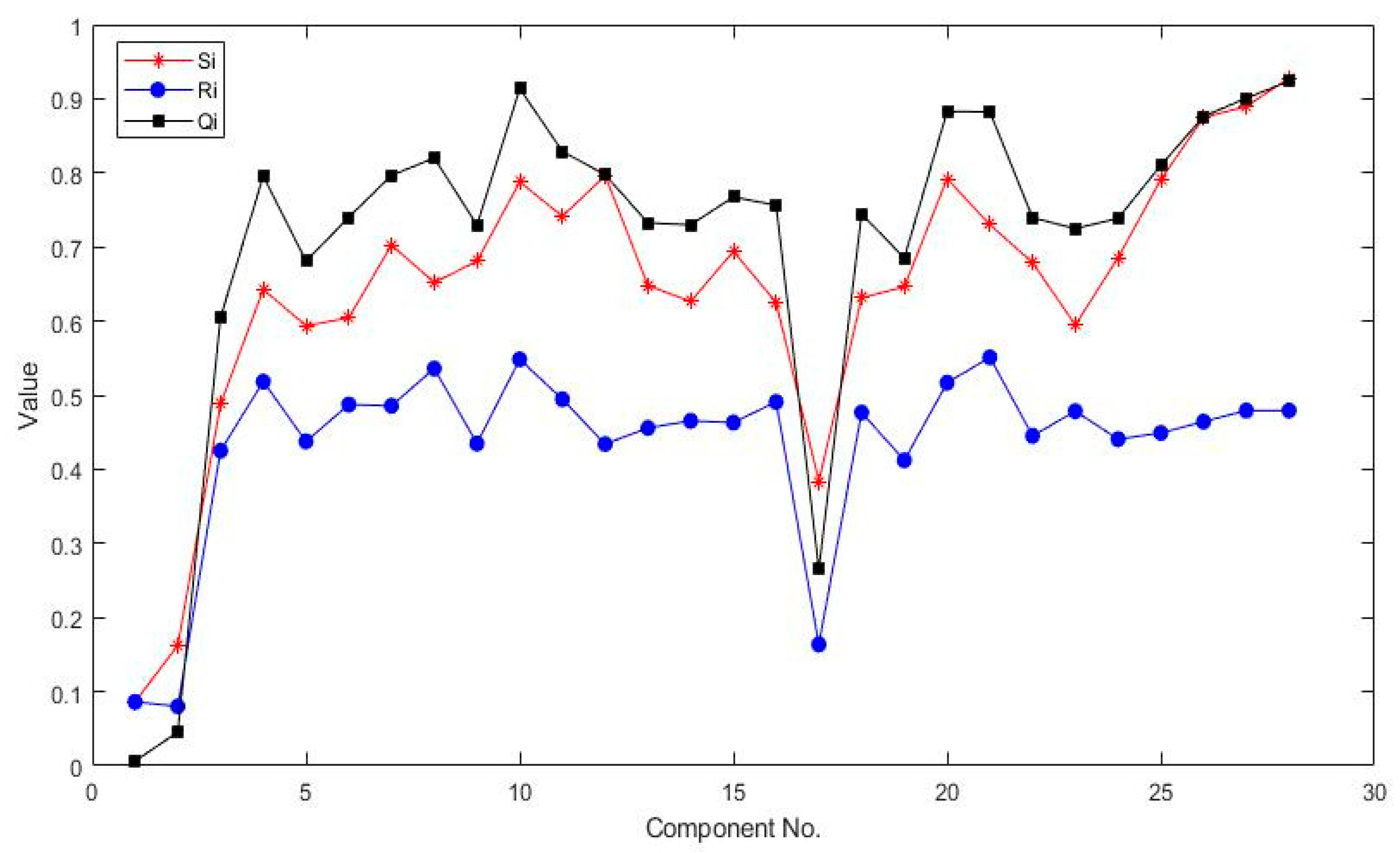
4.1. Calculation of the Risk Prioritization for Railway Train Bogie System

Step 1: Determine and aggregate the FMEA decision value.
Bogie system is one of the most major complex mechatronic part of railway train and can be easily prone to fail. Bogie system can account for a substantial 21.1% based on accumulation of failure data in a couple years [47]. In this paper, a specific railway train bogie system is applied to cope with the proposed FMEA model. Twenty-eight components and seventy-three failure modes are selected for the calculation, which can be Ai (i = 1, 2, …, 28) and FMis (is = 1, 2, …, t, i*is = 73). The components and failure modes can be provided in Table 4 and Table 5, respectively. A FMEA team consists of three members: design manufacturer, train crew and maintenance personnel. They are invited to give the risk score of the failure mode under risk factor O, S and D, and can be expressed by DMk (k = 1, 2, 3).
Based on the Table 1, Table 2 and Table 3, every FMEA team member gives the risk score of the failure mode FMis under the risk factor O, S and D. Table 6 provides the risk score of partial failure modes. Then, importance weights of the FMEA team member can be calculated as 0.2822, 0.3268 and 0.3910 under risk factor O, 0.2455, 0.2406 and 0.5139 under risk factor S and 0.3678, 0.3538 and 0.2784 under risk factor D, respectively. As a result, the aggregated risk score of partial failure modes can be obtained according to Equations (20)–(22) in Section 3.1. Table 7 provides the aggregated risk score of partial failure modes.
Step 2: Determine the cumulative prospect value of each component.
On account of the aggregated risk score of all the failure modes, the reference points under risk factor O, S and D can be determined as ((0.21,0.25,0.37), (0.74,1.0,1.0)), ((0.45,0.55,0.65), (0.45,0.55,0.65)) and ((0.33,0.42,0.52), (0.58,1.0,1.0)), respectively. Then, the gain or loss matrix of failure modes can be obtained based on the Hamming distance between the aggregated risk scores and reference points. Table 8 provides the gain or loss matrix of partial failure modes.
According to the increasing ranking order of gain or loss value of the failure modes for a component, the cumulative prospect weight of each failure mode can be determined in accordance with Equations (26) and (27) in Section 3.2. The cumulative prospect weight of partial failure modes can be shown in Table 9. Thus, the cumulative prospect value of each component can be obtained based on the gain or loss matrix and cumulative prospect weight of failure modes. Table 10 provides the cumulative prospect value of partial bogie system components.
Step 3: Determine the component risk prioritization.
Based on the Equation (28) to Equation (30), we can obtain the weight under risk factor O, S and D as 0.25, 0.18 and 0.57. Then, the maximizing group utility Si, minimizing individual regret Ri and compromise solution Qi can be determined by the VIKOR approach, which can be shown in Figure 2. Table 11 provides the Si, Ri and Qi value of partial bogie system components. Therefore, the risk ranking and prioritization order can be obtained by the increasing order of Qi value.
On the basis of the increasing order of the compromise solution Qi of bogie system components, the risk prioritization ranking result of the top ten components can be Frame assembly > Axle > Drawbar > Wheel > Bearing > Central axis > Parking brake unit > Air spring > Gearbox assembly > Anti-rolling torsion bar. Consequently, the component frame assembly has the top risk prioritization, because frame assembly is the main body of railway train bogie system. Any failures will cause the derailment of the train and results in irretrievable damage. Thus, reliability design of the frame assembly has been always attached great importance.
Furthermore, the crack of axle and drawbar can also lead to the derailment of the train. The microcrack of axle and drawbar can cause the decline of the railway train operation stability and endanger the safety of passengers. The wear of the drawbar counts a large proportion of the fault record and sometimes affect the railway train operation. As a consequence, the component axle and drawbar has the second and third risk prioritization.
In addition, the parking brake unit is an important component to prevent sliding at the parking time when passengers are getting on and off the train. Once the parking brake fails, it can bring about train sliding, and subsequently, passenger injuries. Therefore, FMEA team members give it a high-risk score, and the parking brake has the seventh risk prioritization.

4.2. Comparisons and Discussion

To verify the efficiency of the extended FMEA model, a comparison study is performed with other approaches based on the example mentioned above. The extended FMEA model based on cumulative prospect theory and type-2 intuitionistic fuzzy VIKOR approach has been proposed to improve the accuracy of conventional FMEA by considering the uncertainty, experts’ risk sensitiveness and decision-making psychological behavior. As a result, the conventional FMEA model (conventional model), the multilevel FMEA based on VIKOR model (multilevel VIKOR model), multilevel FMEA with TFNIFS VIKOR model (multilevel TFNIFS VIKOR model) and FMEA with cumulative prospect theory, TFNIFS and TOPSIS model (CPT TFNIFS TOPSIS model) are selected for comparison study to find out the advantages of the proposed FMEA model. The risk prioritization outcomes of the illustrative models are represented in Figure 3.
As shown in Figure 3, the overall prioritization trend of the proposed model essentially agrees with the illustrative models. There are some differences among these models, and the explanations can be given as follows.
The first comparison study is conducted with the outcome derived based on the conventional FMEA model. There are significant differences between the risk prioritization outcomes by the two FMEA models. For instance, the component primary spring has the second risk prioritization in the conventional model, however, it ranks thirteenth when the proposed model is used. The failure of the primary spring practically affects the passenger comfort instead of operation safety. Moreover, the component central axis and drawbar has the fourteenth and fifteenth risk prioritization in the conventional model, which is inconsistent with the actual situation. Central axis and drawbar are the crucial components associated with the safety operation. Based on the proposed model, central axis and drawbar ranks sixth and third, respectively. Therefore, the outcome derived from the conventional model can be inaccurate to some extent. The inaccurate outcomes can be explained as follows:
  • The uncertainty, experts’ risk sensitiveness and decision-making psychological behavior are not considered in the conventional model.
  • The multiplication of risk factor O, S and D can be questionable.
The second comparative analysis is performed with the outcome obtained by the multilevel VIKOR model. There are also numerous distinctions between the two models. For example, the major difference is that the component frame assembly ranks fifth in the multilevel VIKOR model. However, it has the top risk prioritization when the proposed method is adopted, which is consistent with the other three models. In addition, the component primary spring still has the second risk prioritization in the multilevel VIKOR model and is inconsistent with the actual situation. Furthermore, the component axle box body and traction motor have the eighth and seventh risk prioritization in the multilevel VIKOR model, respectively. The failure of axle box body merely affects the passenger comfort and the failure of traction motor will decline the operation stability. According to the proposed model, the axle box body and traction motor rank seventeenth and fifteenth, respectively, which is consistent with the actual situation. The component brake pad has a significant relationship with the operation safety. It ranks eleventh in the proposed model while it barely ranks twenty-second in the multilevel VIKOR model. As a result, the distinction between the two models is that the multilevel VIKOR model considers the VIKOR for multiplication of risk factors but does not think about the uncertainty, experts’ risk sensitiveness and decision-making psychological behavior.
The third comparative analysis is implemented with multilevel TFNIFS VIKOR model. The major difference between the two models is that the component central axis and drawbar has the eighteenth and twenty-first risk prioritization in the multilevel TFNIFS VIKOR model, respectively, and is inconsistent with the actual situation. Moreover, the component air spring has the twenty-second risk prioritization in the multilevel TFNIFS VIKOR model while it ranks eighth in the proposed model. The air spring is the significant component related to operation safety, that needs much attention to keep its reliability. Consequently, the difference between the two models indicates the importance of considering the experts’ risk sensitiveness and decision-making psychological behavior in risk analysis. The last comparative analysis is carried out with CPT TFNIFS TOPSIS model. From Figure 3, the two models share the same risk prioritization about the top four components. However, the risk prioritization of the component air spring and anti-rolling torsion bar in the CPT TFNIFS TOPSIS model vary significantly with the outcomes in the proposed model. As important as air spring, the anti-rolling torsion bar ensure the operation safety when train is travelling and negotiating curve. Air spring and anti-rolling torsion bar ranks eighth and tenth when proposed method is adopted. However, air spring and anti-rolling torsion bar ranks fifteenth and nineteenth in the CPT TFNIFS TOPSIS model, respectively. Hence, the similarities between the two models are that they both consider the same FMEA framework with the MCDM method, uncertainty, experts’ risk sensitiveness and decision-making psychological behavior. Nevertheless, the difference between them is that the VIKOR approach is adopted as the MCDM method in the proposed model as opposed to TOPSIS for the other. Fei et al and Hsu [30,31] illustrates the superiority and flexibility of the VIKOR approach compared with TOPSIS.
Therefore, the comparison studies mentioned above confirm the validity of the proposed FMEA model. The improvement of the enhanced FMEA model based on type-2 intuitionistic fuzzy numbers, VIKOR and cumulative prospect theory can well cope with uncertainty, experts’ risk sensitiveness, decision-making psychological behavior and risk factor fusion problem for the railway train risk prioritization.

5. Conclusions

In this paper, an extended FMEA model is proposed for the railway train risk prioritization based on cumulative prospect theory and type-2 intuitionistic fuzzy VIKOR approach. Firstly, the FMEA framework is applied to examine the vital and risky failure modes and components for the railway train operation. Then, the three risk factors O, S and D are evaluated based on the triangle fuzzy number intuitionistic fuzzy numbers to handle the uncertainty in the risk evaluation for each failure mode. Next, cumulative prospect theory is utilized because it can take into account the FMEA team members’ risk sensitiveness and psychological behavior in the analysis process. Then, TFNIFG operator is applied as the reference point to determine the cumulative prospect value of each failure mode. In addition, the VIKOR method is used for information fusion of the risk factor O, S and D. Furthermore, the entropy weighting method is also adopted to determine FMEA team members’ importance weights and risk factor weights. Finally, the risk prioritization of each component can be obtained. An illustrative example of railway train bogie system is performed to demonstrate the effectiveness of the proposed FMEA model.
Based on the calculation outcome, a comparison study is also carried out with other approaches to validate the effectiveness of the enhanced FMEA model. In accordance with the comparison study, it found that the proposed FMEA model can provide more reasonable and precise results for the railway train risk prioritization.
In regard to future research directions, it is recommended that the multiplication problems for the different risk factors should be handled not only by the MCDM method, but also by evidence theory. In addition, the dynamic FMEA model can be integrated into this problem by considering the full life-cycle activities of the railway train. Furthermore, we will extend the cumulative prospect theory with a number of reference points by taking into account different dimensional risk information.

Author Contributions

Conceptualization, Y.F. and Y.Q.; methodology, Y.F. and W.W.; software, Y.F.; validation, Y.F., Y.Q. and W.W.; formal analysis, L.J.; investigation, Y.F. and Y.Q.; resources, Y.F. and Y.Q.; data curation, Y.Q.; writing—original draft preparation, Y.F.; writing—review and editing, Y.F. and X.L.; visualization, Y.F.; supervision, Y.Q.; project administration, Y.Q.; funding acquisition, Y.Q. All authors have read and agreed to the published version of the manuscript.

Funding

The work was supported by the National Science Foundation of China (NSFC) (61833002).

Acknowledgments

The authors wish to thank the anonymous reviewers for the valuable suggestions and comments which improved the quality of this paper.

Conflicts of Interest

The authors declare no conflict of interest.

References

  1. Vuille, F.; Hofstetter, R.; Mossi, M. Assessing Global RAMS Performance of Large-Scale Complex Systems: Application to Innovative Transport Systems; Science Press: Beijing, China, 2004; Volume 4, pp. 1724–1732. [Google Scholar]
  2. Qazizadeh, A.; Stichel, S.; Persson, R. Proposal for systematic studies of active suspension failures in rail vehicles. Proc. Inst. Mech. Eng. Part F J. Rail Rapid Transit 2018, 232, 199–213. [Google Scholar] [CrossRef]
  3. Zhang, X.G.; Li, Y.L.; Ran, Y.; Zhang, G.B. A Hybrid Multilevel FTA-FMEA Method for a Flexible Manufacturing Cell Based on Meta-Action and TOPSIS. IEEE Access 2019, 7, 110306–110315. [Google Scholar] [CrossRef]
  4. Tooranloo, H.S.; Ayatollah, A.S. Pathology the Internet Banking Service Quality Using Failure Mode and Effect Analysis in Interval-Valued Intuitionistic Fuzzy Environment. Int. J. Fuzzy Syst. 2017, 19, 109–123. [Google Scholar] [CrossRef]
  5. Efe, B. Analysis of operational safety risks in shipbuilding using failure mode and effect analysis approach. Ocean Eng. 2019, 187, 9. [Google Scholar] [CrossRef]
  6. Mohsen, O.; Fereshteh, N. An extended VIKOR method based on entropy measure for the failure modes risk assessment—A case study of the geothermal power plant (GPP). Saf. Sci. 2017, 92, 160–172. [Google Scholar] [CrossRef]
  7. Wang, W.Z.; Liu, X.W.; Liu, S.L. Failure mode and effect analysis for machine tool risk analysis using extended gained and lost dominance score method. IEEE Trans. Reliab. 2019, 69, 945–967. [Google Scholar] [CrossRef]
  8. Biswas, T.K.; Zaman, K. A Fuzzy-Based Risk Assessment Methodology for Construction Projects Under Epistemic Uncertainty. Int. J. Fuzzy Syst. 2019, 21, 1221–1240. [Google Scholar] [CrossRef]
  9. Dincer, H.; Yuksel, S. Comparative Evaluation of BSC-Based New Service Development Competencies in Turkish Banking Sector with the Integrated Fuzzy Hybrid MCDM Using Content Analysis. Int. J. Fuzzy Syst. 2018, 20, 2497–2516. [Google Scholar] [CrossRef]
  10. Liang, Y.Y.; Liu, J.; Qin, J.; Tu, Y. An Improved Multi-granularity Interval 2-Tuple TODIM Approach and Its Application to Green Supplier Selection. Int. J. Fuzzy Syst. 2019, 21, 129–144. [Google Scholar] [CrossRef]
  11. Han, W.; Sun, Y.H.; Xie, H.; Che, Z.M. Hesitant Fuzzy Linguistic Group DEMATEL Method with Multi-granular Evaluation Scales. Int. J. Fuzzy Syst. 2018, 20, 2187–2201. [Google Scholar] [CrossRef]
  12. Meng, F.Y.; Chen, X.H.; Zhang, Q. Generalized Hesitant Fuzzy Generalized Shapley-Choquet Integral Operators and Their Application in Decision Making. Int. J. Fuzzy Syst. 2014, 16, 400–410. [Google Scholar]
  13. Teng, F.; Liu, P. Multiple-Attribute Group Decision-Making Method Based on the Linguistic Intuitionistic Fuzzy Density Hybrid Weighted Averaging Operator. Int. J. Fuzzy Syst. 2019, 21, 213–231. [Google Scholar] [CrossRef]
  14. Xue, M.; Fu, C.; Chang, W.J. Determining the Parameter of Distance Measure Between Dual Hesitant Fuzzy Information in Multiple Attribute Decision Making. Int. J. Fuzzy Syst. 2018, 20, 2065–2082. [Google Scholar] [CrossRef]
  15. Yu, S.M.; Wang, J.; Wang, J.Q. An Interval Type-2 Fuzzy Likelihood-Based MABAC Approach and Its Application in Selecting Hotels on a Tourism Website. Int. J. Fuzzy Syst. 2017, 19, 47–61. [Google Scholar] [CrossRef]
  16. Wei, A.P.; Li, D.F.; Jiang, B.Q.; Lin, P.P. The Novel Generalized Exponential Entropy for Intuitionistic Fuzzy Sets and Interval Valued Intuitionistic Fuzzy Sets. Int. J. Fuzzy Syst. 2019, 21, 2327–2339. [Google Scholar] [CrossRef]
  17. Liu, F.; Yuan, X.H. Fuzzy Number Intuitionistic Fuzzy Set. Fuzzy Syst. Math. 2007, 21, 88–91. [Google Scholar]
  18. Chen, D.F.; Zhang, L.; Jiao, J.S. Triangle Fuzzy Number Intuitionistic Fuzzy Aggregation Operators and Their Application to Group Decision Making. In Artificial Intelligence and Computational Intelligence, Aici 2010, Pt Ii; Wang, F.L., Deng, H., Gao, Y., Lei, J., Eds.; Springer: Berlin, Germay, 2010; Volume 6320, pp. 350–357. [Google Scholar]
  19. Liu, H.C.; Chen, X.Q.; Duan, C.Y.; Wang, Y.M. Failure mode and effect analysis using multi-criteria decision making methods: A systematic literature review. Comput. Ind. Eng. 2019, 135, 881–897. [Google Scholar] [CrossRef]
  20. Faiella, G.; Parand, A.; Franklin, B.D.; Chana, P.; Cesarelli, M.; Stanton, N.A.; Sevdalis, N. Expanding healthcare failure mode and effect analysis: A composite proactive risk analysis approach. Reliab. Eng. Syst. Saf. 2018, 169, 117–126. [Google Scholar] [CrossRef] [Green Version]
  21. Wang, W.Z.; Liu, X.W.; Chen, X.Q.; Qin, Y. Risk assessment based on hybrid FMEA framework by considering decision maker’s psychological behavior character. Comput. Ind. Eng. 2019, 136, 516–527. [Google Scholar] [CrossRef]
  22. Fattahi, R.; Khalilzadeh, M. Risk evaluation using a novel hybrid method based on FMEA, extended MULTIMOORA, and AHP methods under fuzzy environment. Saf. Sci. 2018, 102, 290–300. [Google Scholar] [CrossRef]
  23. Blagojevic, A.; Stevic, Z.; Marinkovic, D.; Kasalica, S.; Rajilic, S. A Novel Entropy-Fuzzy PIPRECIA-DEA Model for Safety Evaluation of Railway Traffic. Symmetry 2020, 12, 1479. [Google Scholar] [CrossRef]
  24. Krmac, E.; Djordjević, B. Evaluation of the TCIS Influence on the capacity utilization using the TOPSIS method: Case studies of Serbian and Austrian railways. Oper. Res. Eng. Sci. Theory Appl. 2019, 2, 27–36. [Google Scholar] [CrossRef]
  25. Liu, H.C.; Liu, L.; Liu, N.; Mao, L.X. Risk evaluation in failure mode and effects analysis with extended VIKOR method under fuzzy environment. Expert Syst. Appl. 2012, 39, 12926–12934. [Google Scholar] [CrossRef]
  26. Lo, H.W.; Liou, J.J.H.; Huang, C.N.; Chuang, Y.C. A novel failure mode and effect analysis model for machine tool risk analysis. Reliab. Eng. Syst. Saf. 2019, 183, 173–183. [Google Scholar] [CrossRef]
  27. Mandal, S.; Singh, K.; Behera, R.K.; Sahu, S.K.; Raj, N.; Maiti, J. Human error identification and risk prioritization in overhead crane operations using HTA, SHERPA and fuzzy VIKOR method. Expert Syst. Appl. 2015, 42, 7195–7206. [Google Scholar] [CrossRef]
  28. Li, G.F.; Li, Y.; Chen, C.H.; He, J.L.; Hou, T.W.; Chen, J.H. Advanced FMEA method based on interval 2-tuple linguistic variables and TOPSIS. Qual. Eng. 2020, 32, 653–662. [Google Scholar] [CrossRef]
  29. Opricovic, S.; Tzeng, G.H. Compromise solution by MCDM methods: A comparative analysis of VIKOR and TOPSIS. Eur. J. Oper. Res. 2004, 156, 445–455. [Google Scholar] [CrossRef]
  30. Fei, L.G.; Deng, Y.; Hu, Y. DS-VIKOR: A New Multi-criteria Decision-Making Method for Supplier Selection. Int. J. Fuzzy Syst. 2019, 21, 157–175. [Google Scholar] [CrossRef]
  31. Hsu, W. A Fuzzy Multiple-Criteria Decision-Making System for Analyzing Gaps of Service Quality. Int. J. Fuzzy Syst. 2015, 17, 256–267. [Google Scholar] [CrossRef]
  32. Li, C.B.; Yuan, J.H. A New Multi-attribute Decision-Making Method with Three-Parameter Interval Grey Linguistic Variable. Int. J. Fuzzy Syst. 2017, 19, 292–300. [Google Scholar] [CrossRef]
  33. Li, X.H.; Chen, X.H. Value determination method based on multiple reference points under a trapezoidal intuitionistic fuzzy environment. Appl. Soft Comput. 2018, 63, 39–49. [Google Scholar] [CrossRef]
  34. Liu, Y.; Wang, Y.; Xu, M.Z.; Xu, G.C. Emergency Alternative Evaluation Using Extended Trapezoidal Intuitionistic Fuzzy Thermodynamic Approach with Prospect Theory. Int. J. Fuzzy Syst. 2019, 21, 1801–1817. [Google Scholar] [CrossRef]
  35. Wang, W.Z.; Liu, X.W.; Qin, Y.; Fu, Y. A risk evaluation and prioritization method for FMEA with prospect theory and Choquet integral. Saf. Sci. 2018, 110, 152–163. [Google Scholar] [CrossRef]
  36. Tversky, A.; Kahneman, D. Advances in prospect-theory—Cumulative representation of uncertainty. J. Risk Uncertain. 1992, 5, 297–323. [Google Scholar] [CrossRef]
  37. Zhao, H.R.; Guo, S.; Zhao, H.R. Comprehensive assessment for battery energy storage systems based on fuzzy-MCDM considering risk preferences. Energy 2019, 168, 450–461. [Google Scholar] [CrossRef]
  38. Li, Y.L.; Ying, C.S.; Chin, K.S.; Yang, H.T.; Xu, J. Third-party reverse logistics provider selection approach based on hybrid-information MCDM and cumulative prospect theory. J. Clean. Prod. 2018, 195, 573–584. [Google Scholar] [CrossRef]
  39. Wang, L.; Liu, Q.; Yin, T.L. Decision-making of investment in navigation safety improving schemes with application of cumulative prospect theory. Proc. Inst. Mech. Eng. Part O J. Risk Reliab. 2018, 232, 710–724. [Google Scholar] [CrossRef]
  40. Wu, Y.N.; Xu, C.B.; Zhang, T. Evaluation of renewable power sources using a fuzzy MCDM based on cumulative prospect theory: A case in China. Energy 2018, 147, 1227–1239. [Google Scholar] [CrossRef]
  41. Zhou, L. On Atanassov’s Intuitionistic Fuzzy Sets in the Complex Plane and the Field of Intuitionistic Fuzzy Numbers. IEEE Trans. Fuzzy Syst. 2016, 24, 253–259. [Google Scholar] [CrossRef]
  42. Hang, S.U.; Qian, W.Y. TOPSIS method for multiple attribute decision-making with fuzzy number intuitionistic fuzzy information. J. Bohai Univ. (Nat. Sci. Ed.) 2012, 33, 6–10. [Google Scholar]
  43. Wang, L.; Wang, Y.-M.; Martinez, L. A group decision method based on prospect theory for emergency situations. Inf. Sci. 2017, 418, 119–135. [Google Scholar] [CrossRef]
  44. Cui, X.; He, Z. Application of the fuzzy AHP model based on a new scale method in the financial risk assessment of the listing corporation. Chem. Eng. Trans. 2015, 46, 1231–1236. [Google Scholar] [CrossRef]
  45. Sharizli, A.A.; Rahizar, R.; Karim, M.R.; Saifizul, A.A. New Method for Distance-based Close Following Safety Indicator. Traffic Inj. Prev. 2015, 16, 190–195. [Google Scholar] [CrossRef] [PubMed]
  46. Kersuliene, V.; Zavadskas, E.K.; Turskis, Z. Selection of rational dispute resolution method by applying new step-wise weight assessment ratio analysis (swara). J. Bus. Econ. Manag. 2010, 11, 243–258. [Google Scholar] [CrossRef]
  47. Kou, L.L.; Qin, Y.; Zhao, X.J.; Fu, Y. Integrating synthetic minority oversampling and gradient boosting decision tree for bogie fault diagnosis in rail vehicles. Proc. Inst. Mech. Eng. Part F J. Rail Rapid Transit 2019, 233, 312–325. [Google Scholar] [CrossRef]
Figure 1. Flowchart of the proposed FMEA model.
Entropy 22 01418 g001
Figure 2. Si, Ri and Qi value of bogie system components.
Entropy 22 01418 g002
Figure 3. Risk prioritization order of failure modes of bogie system components.
Entropy 22 01418 g003
Table 1. Linguistic variables for the risk factor occurrence (O).
Linguistic VariablesRankTFNIFNs
Very low1, 2((0.1,0.1,0.2), (0.9,1.0,1.0))
Low3, 4((0.2,0.3,0.4), (0.7,0.8,0.9))
Medium5, 6((0.4,0.5,0.6), (0.5,0.6,0.7))
High7, 8((0.6,0.7,0.8), (0.3,0.4,0.5))
Very high9, 10((0.8,0.9,1.0), (0.1,0.2,0.3))
Table 2. Linguistic variables for the risk factor severity (S).
Linguistic VariablesRankTFNIFNs
Very minor1, 2((0.1,0.1,0.2), (0.9,1.0,1.0))
Minor3, 4((0.2,0.3,0.4), (0.7,0.8,0.9))
Medium5, 6((0.4,0.5,0.6), (0.5,0.6,0.7))
Major7, 8((0.6,0.7,0.8), (0.3,0.4,0.5))
Hazardous9, 10((0.8,0.9,1.0), (0.1,0.2,0.3))
Table 3. Linguistic variables for the risk factor detection (D).
Linguistic VariablesRankTFNIFNs
Very easy1, 2((0.1,0.1,0.2), (0.9,1.0,1.0))
Easy3, 4((0.2,0.3,0.4), (0.7,0.8,0.9))
Medium5, 6((0.4,0.5,0.6), (0.5,0.6,0.7))
Hard7, 8((0.6,0.7,0.8), (0.3,0.4,0.5))
Very hard9, 10((0.8,0.9,1.0), (0.1,0.2,0.3))
Table 4. Bogie system components selected for the calculation.
No.ComponentNo.Component
1Frame assembly15Coupling
2Axle16Traction motor
3Wheel17Drawbar
4Axle box body18Traction frame
5Bearing19Central axis
6Primary spring20Central pin
7Vertical shock absorber21Lateral buffer device
8Lateral stop22Tread Braking Unit
9Air spring23Parking brake unit
10Height adjustment device24Brake pad
11Differential pressure valve25Flange lubrication device
12Lateral shock absorber26Grounding device
13Anti-rolling torsion bar27RFID
14Gearbox assembly28Temperature sensor
Table 5. Bogie system components selected for the calculation.
No.Component No.Failure ModeNo.Component No.Failure Mode
11Microcrack3814Oil leak
21Crack3914Low oil level
32Microcrack4014Microcrack
42Crack4114Crack
53Crack4214Abnormal sound
63Tread scratch4314Gear damage
73Tread peeling4414Gear crack
83Tread crack4515Microcrack
93Wheel wear4615Crack
104Microcrack4715Loosening
114Wear4816Abnormal vibration
124Crack4916Over-temperature
134Abnormal temperature5016Bearing crack
145Scratch5116Internal wiring damage
155Microcrack5216Stop turning
165Crack5317Crack
175Abnormal temperature5417Microcrack
186Wear5517Wear
196Microcrack5618Crack
206Crack5718Microcrack
217Loosening5819Crack
227Oil leak5919Microcrack
238Microcrack6020Wear
248Crushed6120Microcrack
259Scratch6220Crack
269Crack6321Crack
279Air leak6421Microcrack
2810Block6522Brake failure
2910Loosening6623Brake failure
3011Block6724Wear
3112Oil leak6824Unable to brake
3212Ageing6925No oil supply
3313Loosening7025Stent crack
3413Deformation7126Open circuit
3513Microcrack7227Unable to transmit
3613Crack7328Unable to detect
3714Abnormal oil
Table 6. Bogie system components selected for the calculation.
No.Component No.pDM1 for Factor ODM1 for Factor SDM1 for Factor DDM2 for Factor ODM2 for Factor SDM2 for Factor DDM3 for Factor ODM3 for Factor SDM3 for Factor D
320.9((0.6,0.7,0.8), (0.3,0.4,0.5))((0.6,0.7,0.8), (0.3,0.4,0.5))((0.6,0.7,0.8), (0.3,0.4,0.5))((0.4,0.5,0.6), (0.5,0.6,0.7))((0.6,0.7,0.8), (0.3,0.4,0.5))((0.6,0.7,0.8), (0.3,0.4,0.5))((0.4,0.5,0.6), (0.5,0.6,0.7))((0.6,0.7,0.8), (0.3,0.4,0.5))((0.4,0.5,0.6), (0.5,0.6,0.7))
420.1((0.1,0.1,0.2), (0.9,1.0,1.0))((0.8,0.9,1.0), (0.1,0.2,0.3))((0.6,0.7,0.8), (0.3,0.4,0.5))((0.1,0.1,0.2), (0.9,1.0,1.0))((0.8,0.9,1.0), (0.1,0.2,0.3))((0.6,0.7,0.8), (0.3,0.4,0.5))((0.1,0.1,0.2), (0.9,1.0,1.0))((0.8,0.9,1.0), (0.1,0.2,0.3))((0.6,0.7,0.8), (0.3,0.4,0.5))
530.05((0.6,0.7,0.8), (0.3,0.4,0.5))((0.6,0.7,0.8), (0.3,0.4,0.5))((0.6,0.7,0.8), (0.3,0.4,0.5))((0.6,0.7,0.8), (0.3,0.4,0.5))((0.4,0.5,0.6), (0.5,0.6,0.7))((0.4,0.5,0.6), (0.5,0.6,0.7))((0.4,0.5,0.6), (0.5,0.6,0.7))((0.4,0.5,0.6), (0.5,0.6,0.7))((0.4,0.5,0.6), (0.5,0.6,0.7))
630.05((0.4,0.5,0.6), (0.5,0.6,0.7))((0.8,0.9,1.0), (0.1,0.2,0.3))((0.6,0.7,0.8), (0.3,0.4,0.5))((0.2,0.3,0.4), (0.7,0.8,0.9))((0.8,0.9,1.0), (0.1,0.2,0.3))((0.4,0.5,0.6), (0.5,0.6,0.7))((0.2,0.3,0.4), (0.7,0.8,0.9))((0.8,0.9,1.0), (0.1,0.2,0.3))((0.4,0.5,0.6), (0.5,0.6,0.7))
730.05((0.2,0.3,0.4), (0.7,0.8,0.9))((0.6,0.7,0.8), (0.3,0.4,0.5))((0.6,0.7,0.8), (0.3,0.4,0.5))((0.2,0.3,0.4), (0.7,0.8,0.9))((0.6,0.7,0.8), (0.3,0.4,0.5))((0.6,0.7,0.8), (0.3,0.4,0.5))((0.1,0.1,0.2), (0.9,1.0,1.0))((0.4,0.5,0.6), (0.5,0.6,0.7))((0.4,0.5,0.6), (0.5,0.6,0.7))
830.84((0.8,0.9,1.0), (0.1,0.2,0.3))((0.4,0.5,0.6), (0.5,0.6,0.7))((0.4,0.5,0.6), (0.5,0.6,0.7))((0.8,0.9,1.0), (0.1,0.2,0.3))((0.4,0.5,0.6), (0.5,0.6,0.7))((0.4,0.5,0.6), (0.5,0.6,0.7))((0.8,0.9,1.0), (0.1,0.2,0.3))((0.4,0.5,0.6), (0.5,0.6,0.7))((0.4,0.5,0.6), (0.5,0.6,0.7))
930.01((0.1,0.1,0.2), (0.9,1.0,1.0))((0.8,0.9,1.0), (0.1,0.2,0.3))((0.6,0.7,0.8), (0.3,0.4,0.5))((0.1,0.1,0.2), (0.9,1.0,1.0))((0.8,0.9,1.0), (0.1,0.2,0.3))((0.8,0.9,1.0), (0.1,0.2,0.3))((0.1,0.1,0.2), (0.9,1.0,1.0))((0.8,0.9,1.0), (0.1,0.2,0.3))((0.8,0.9,1.0), (0.1,0.2,0.3))
Table 7. Aggregated risk score of partial failure modes.
No.Component No.pOSD
320.9((0.45,0.55,0.65), (0.44,0.54,0.64))((0.6,0.7,0.8), (0.3,0.4,0.5))((0.54,0.64,0.74), (0.35,0.45,0.55))
420.1((0.1,0.1,0.2), (0.9,1.0,1.0))((0.8,0.9,1.0), (0.1,0.2,0.3))((0.6,0.7,0.8), (0.3,0.4,0.5))
530.05((0.52,0.62,0.72), (0.37,0.47,0.57))((0.45,0.55,0.65), (0.44,0.54,0.64))((0.47,0.57,0.67), (0.42,0.52,0.62))
630.05((0.26,0.36,0.46), (0.64,0.74,0.84))((0.8,0.9,1.0), (0.1,0.2,0.3))((0.47,0.57,0.67), (0.42,0.52,0.62))
730.05((0.16,0.22,0.32), (0.77,0.87,0.93))((0.49,0.59,0.69), (0.40,0.50,0.60))((0.54,0.64,0.74), (0.35,0.45,0.55))
830.84((0.8,0.9,1.0), (0.1,0.2,0.3))((0.4,0.5,0.6), (0.5,0.6,0.7))((0.4,0.5,0.6), (0.5,0.6,0.7))
930.01((0.1,0.1,0.2), (0.9,1.0,1.0))((0.8,0.9,1.0), (0.1,0.2,0.3))(0.72,0.82,0.92), (0.17,0.27,0.37)
Table 8. Gain or loss matrix of partial failure modes.
No.Component No.pOSD
320.90.380.190.37
420.1−0.280.410.44
530.050.45−0.03−0.69
630.050.170.40−0.69
730.05−0.200.080.38
830.840.71−0.14−0.51
930.01−0.280.400.56
Table 9. Cumulative prospect weight of partial failure modes.
No.Component No.pOSD
320.90.710.810.81
420.10.170.190.19
530.050.050.060.11
630.050.070.090.06
730.050.090.050.09
830.840.640.710.66
930.010.040.050.06
Table 10. Cumulative prospect weight of partial components.
Component No.OSD
10.468144−0.04211−0.39385
20.298719−0.09364−0.60525
30.281249−0.22827−0.42217
40.336425−0.1147−0.5351
50.030094−0.15011−0.5314
60.052312−0.0584−0.46359
70.098971−0.40377−0.41591
80.468144−0.04211−0.39385
90.298719−0.09364−0.60525
Table 11. Si, Ri and Qi value of partial components.
Component No.OSD
10.468144−0.04211−0.39385
20.298719−0.09364−0.60525
30.281249−0.22827−0.42217
40.336425−0.1147−0.5351
50.030094−0.15011−0.5314
60.052312−0.0584−0.46359
70.098971−0.40377−0.41591
80.468144−0.04211−0.39385
90.298719−0.09364−0.60525
Publisher’s Note: MDPI stays neutral with regard to jurisdictional claims in published maps and institutional affiliations.

