A Labeling Method for Financial Time Series Prediction Based on Trends


Abstract
:1. Introduction
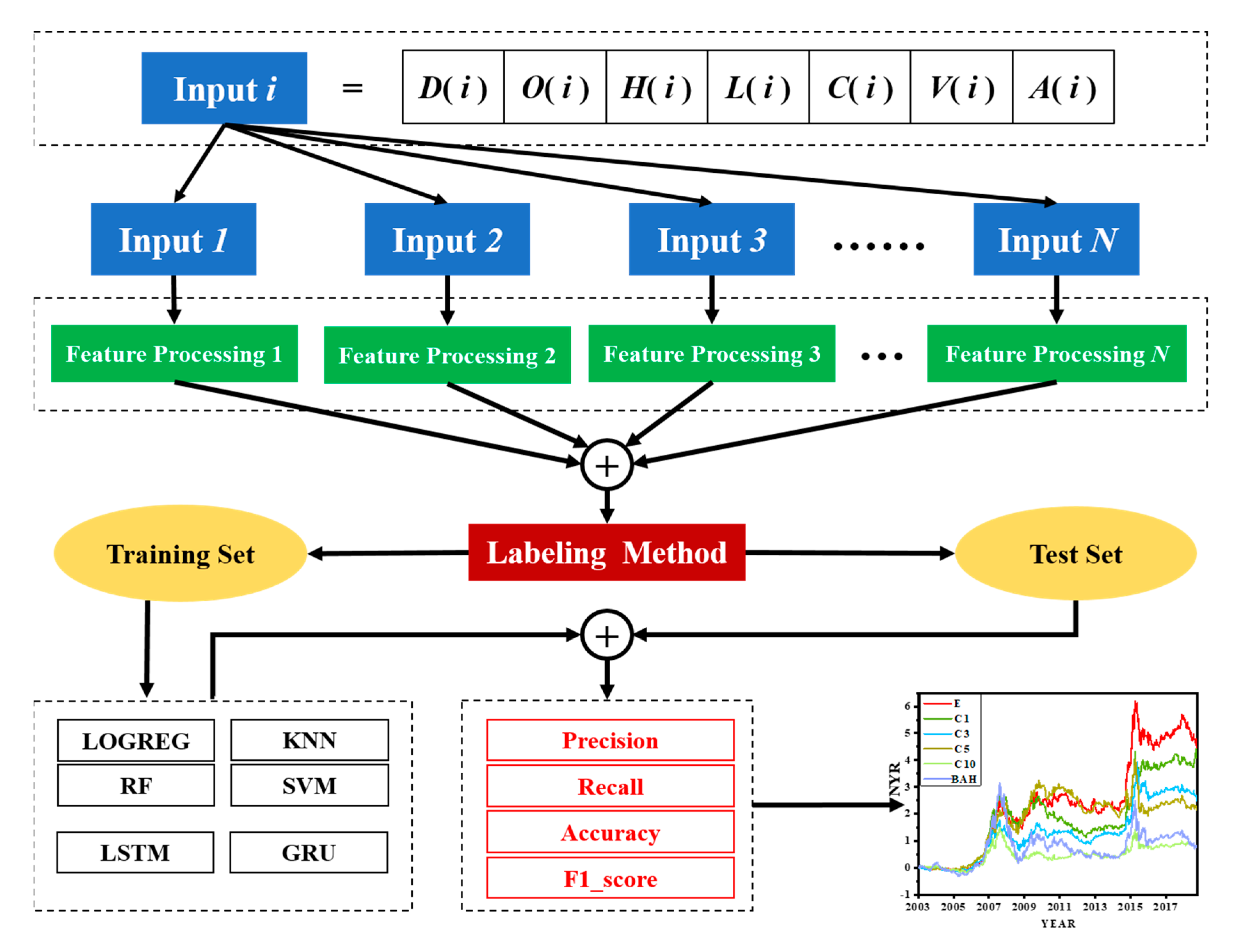
2. Methodology
2.1. Learning Algorithms
2.1.1. Logistic Regression (LOGREG)
2.1.2. Random Forest (RF)
2.1.3. KNN
2.1.4. Support Vector Machine (SVM)
2.1.5. Long Short-Term Memory (LSTM)
2.1.6. Gated Recurrent Unit (GRU)
2.2. Vector Space Reconstruction
2.2.1. Vector Dimension Expansion
2.2.2. Feature Processing Method without Look-Ahead Bias
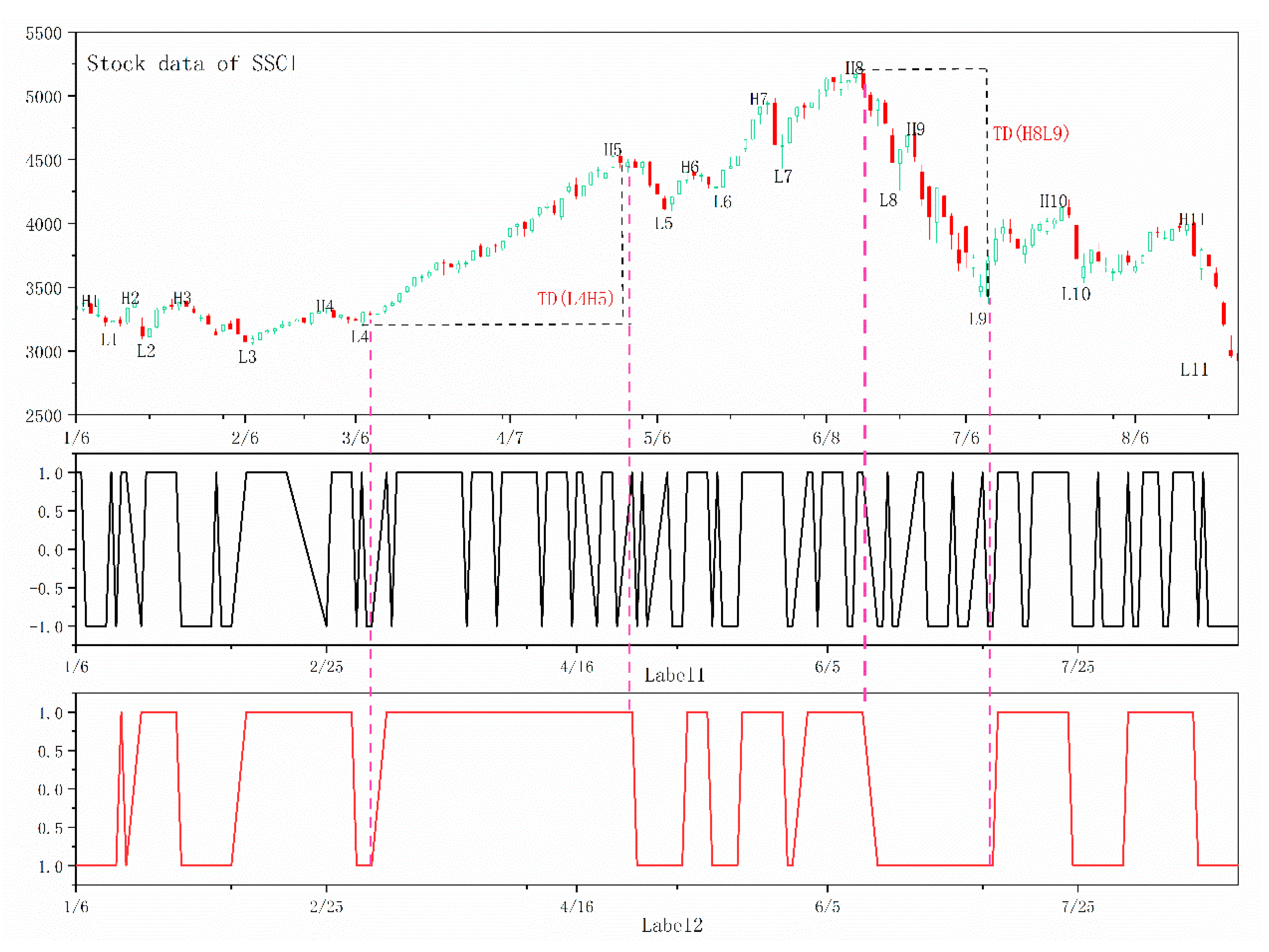
2.3. Definition of Continuous Trend Labeling
| Algorithm 1. Auto-Labeling Data for CTL |
| Input: Original Time series data,>0, which represents the proportion threshold parameter of the trend definition |
| Output: The label vector |
| Initialization of related variables: |
| FP=x1, which represents the first price obtained by the algorithm; xH =x1, used to mark the highest price; HT=t1, used to mark the time when the highest price occurs; xL =x1, used to mark the lowest price; LT=t1, used to mark the time when the lowest price occurs; Cid=0, used to mark the current direction of labeling; FP_N =0, the index of the highest or lowest point obtained initially. |
| fori = 1:N if (xi > FP + x1*) Set [xH, HT, FP_N, Cid ] = [ xi, ti, i,1] and end for if (xi < FP- x1*) Set [xL, LT, FP_N, Cid ] = [ xi, ti, i, −1] and end for end for i for i = FP_N+1:N if (Cid > 0) if (xi > xH) Set [xH, HT] = [ xi, ti ] if (xi < xH - xH* and LT <= HT) for j = 1:N if (tj > LT and tj <= HT) Set yj = 1 end for j Set [xL, LT, Cid] = [ xi, ti, −1] if (Cid < 0) if (xi < xL) Set [xL, LT] = [ xi, ti ] if (xi > xL + xL * and HT <= LT) for j = 1:N if (tj > HT and tj < = LT) Set yj = −1 end for j Set[xH, HT, Cid] = [ xi, ti, 1] end for i |
3. Research Design
3.1. Data Description
3.2. Input Setup
3.3. Comparison Experiments
3.4. Statistical Metrics
4. Experimental Results
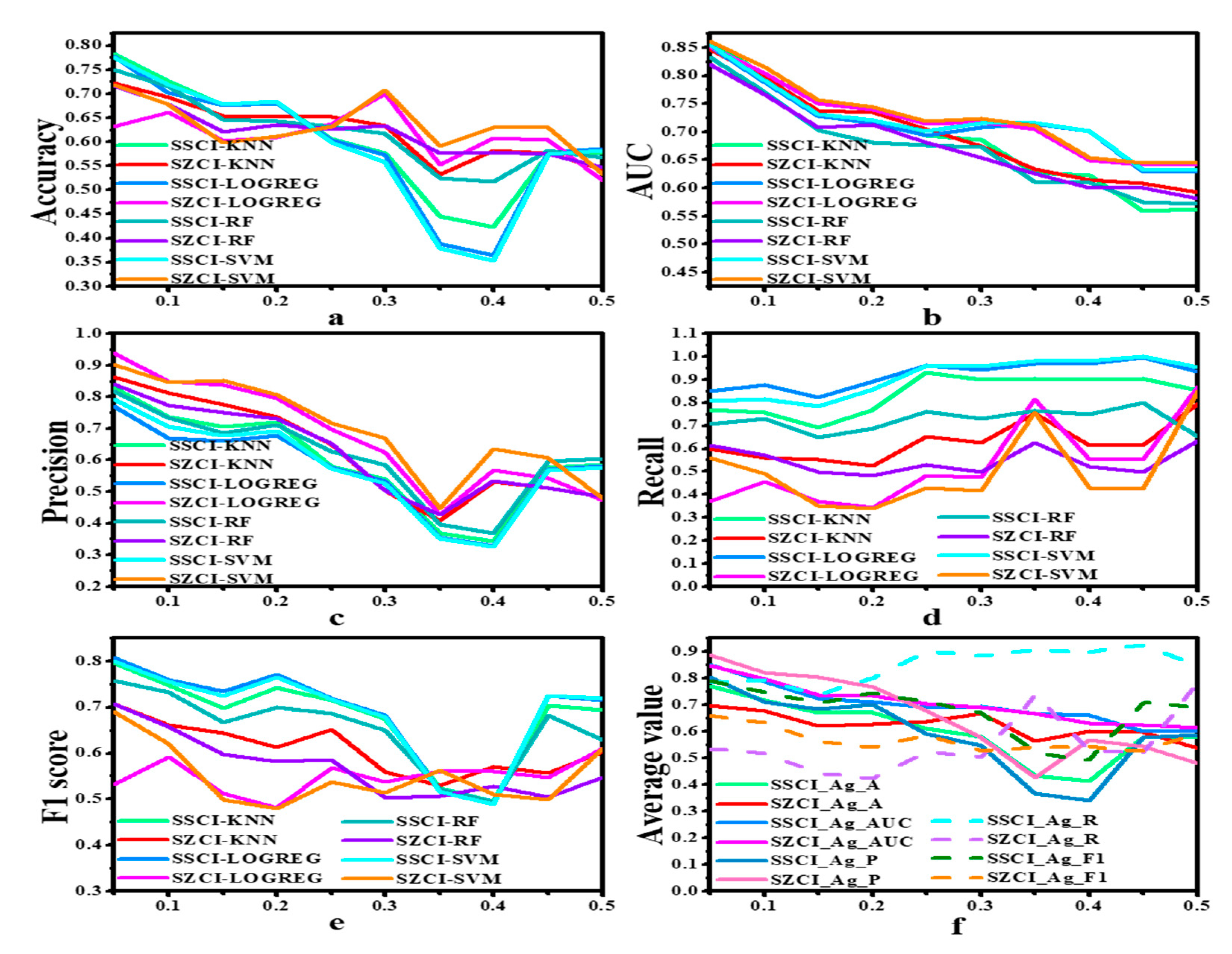
4.1. Analysis of Threshold Parameters
4.2. Classification Results and Analysis
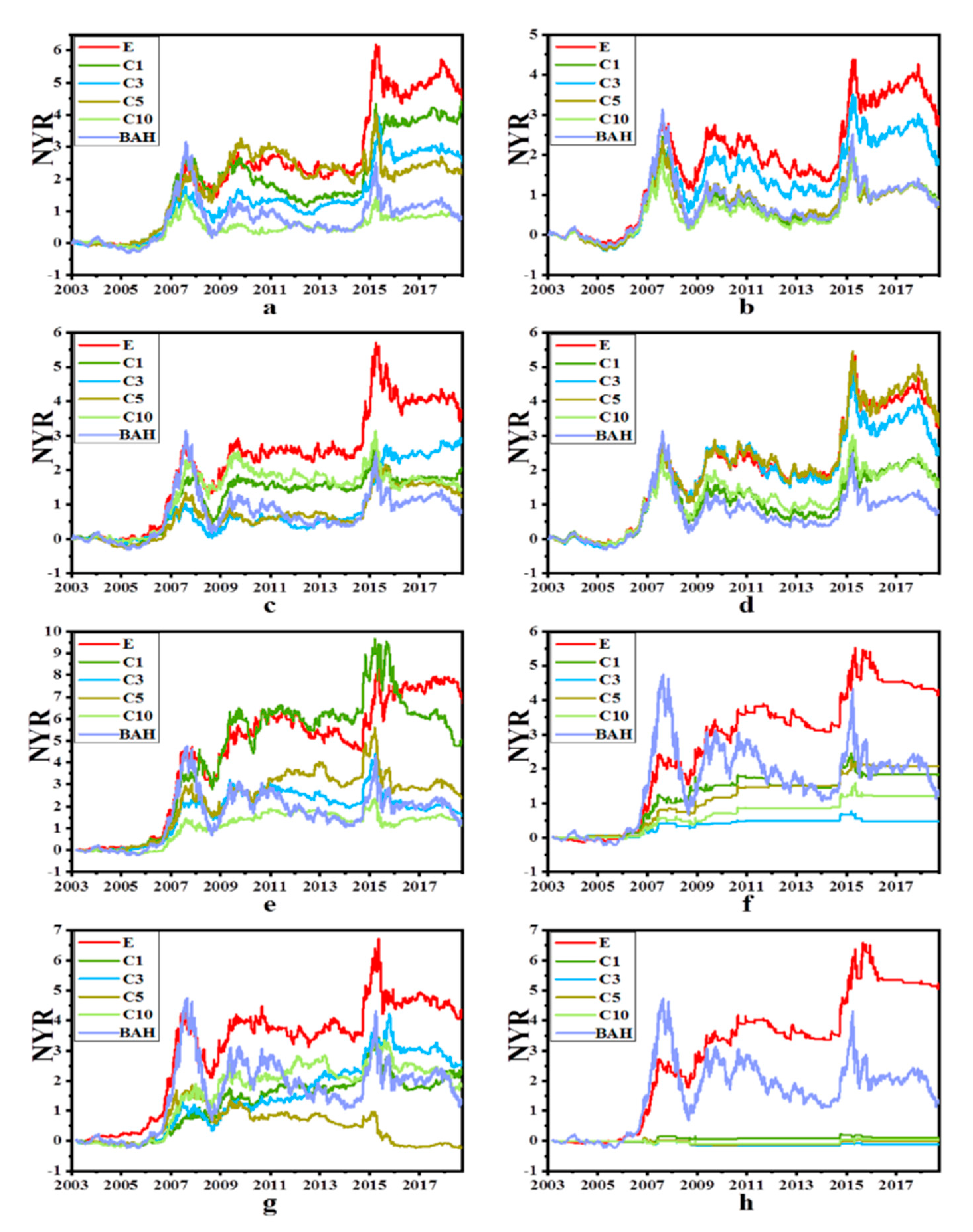
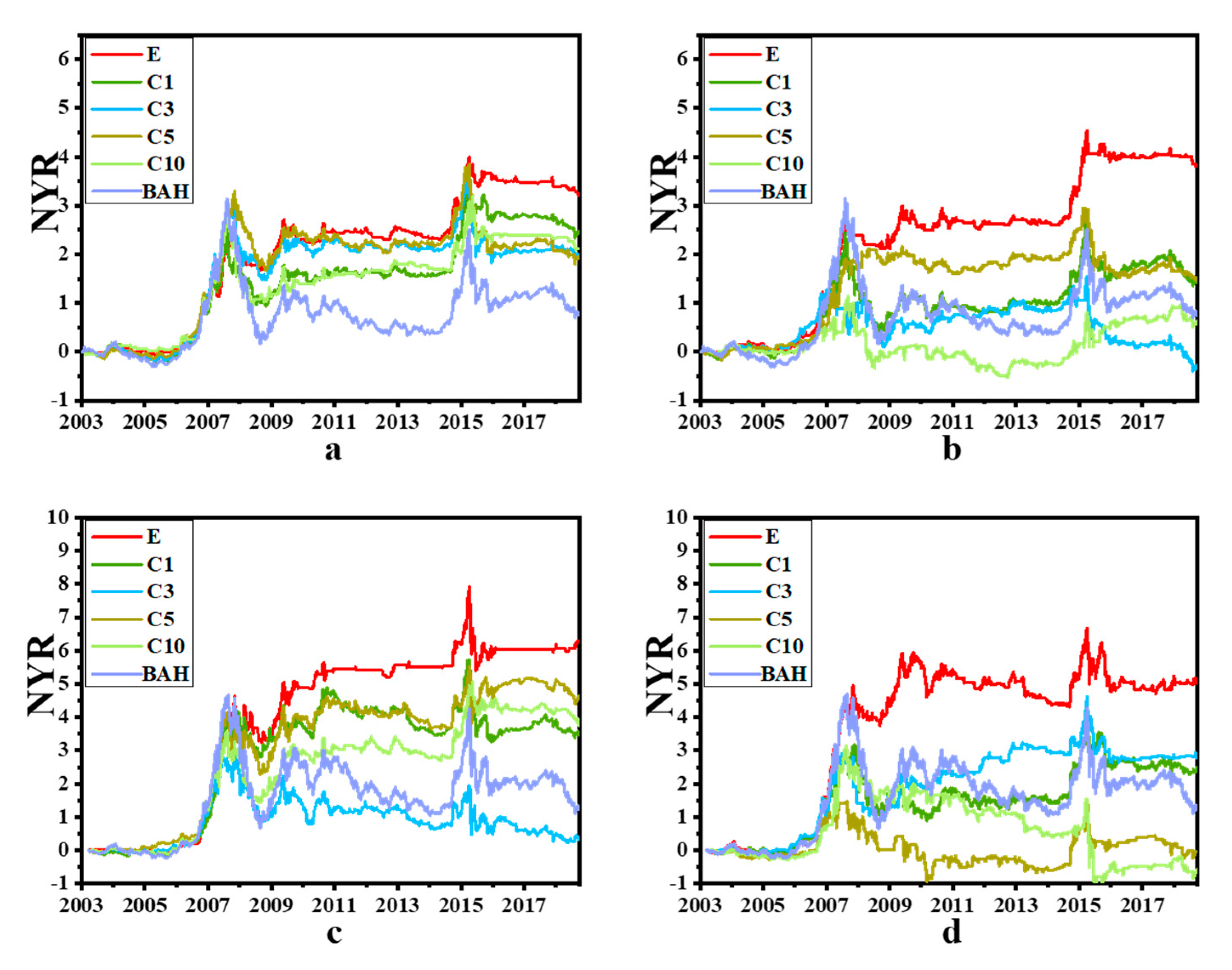
4.3. Implementation of Strategies
5. Conclusions
Author Contributions
Funding
Conflicts of Interest
References
- Li, J.; Shang, P.; Zhang, X. Financial Time Series Analysis Based on Fractional and Multiscale Permutation Entropy. Commun. Nonlinear Sci. Numer. Simul. 2019, 78, 104880–104892. [Google Scholar] [CrossRef]
- Sapankevych, N.I.; Sankar, R. Time Series Prediction Using Support Vector Machines: A Survey. IEEE Comput. Intell. Mag. 2009, 4, 24–38. [Google Scholar] [CrossRef]
- Liu, P.; Liu, J.; Wu, K. Cnn-Fcm: System Modeling Promotes Stability of Deep Learning in Time Series Prediction. Knowl. Based Syst. 2020, 203, 106081–106093. [Google Scholar] [CrossRef]
- Yang, R.; Yu, L.; Zhao, Y.; Yu, H.; Xu, G.; Wu, Y.; Liu, Z. Big Data Analytics for Financial Market Volatility Forecast Based on Support Vector Machine. Int. J. Inf. Manag. 2020, 50, 452–462. [Google Scholar] [CrossRef]
- Akyildirim, E.; Corbet, S.; Efthymiou, M.; Guiomard, C.; O’Connell, J.F.; Sensoy, A. The Financial Market Effects of International Aviation Disasters. Int. Rev. Financ. Anal. 2020, 69, 101468–101485. [Google Scholar] [CrossRef]
- Göçken, M.; Özçalıcı, M.; Boru, A.; Dosdoğru, A.T. Integrating Metaheuristics and Artificial Neural Networks for Improved Stock Price Prediction. Expert Syst. Appl. 2016, 44, 320–331. [Google Scholar] [CrossRef]
- Hu, Y.; Valera, H.G.A.; Oxley, L. Market Efficiency of the Top Market-Cap Cryptocurrencies: Further Evidence from a Panel Framework. Financ. Res. Lett. 2019, 31, 138–145. [Google Scholar] [CrossRef]
- Kristoufek, L. On Bitcoin Markets (in) Efficiency and Its Evolution. Phys. A Stat. Mech. Its Appl. 2018, 503, 257–262. [Google Scholar] [CrossRef]
- Sigaki, H.Y.; Perc, M.; Ribeiro, H.V. Clustering Patterns in Efficiency and the Coming-of-Age of the Cryptocurrency Market. Sci. Rep. 2019, 9, 1–9. [Google Scholar] [CrossRef]
- Liu, B.; Xia, X.; Xiao, W. Public Information Content and Market Information Efficiency: A Comparison between China and the US. China Econ. Rev. 2020, 60, 101405–101417. [Google Scholar] [CrossRef]
- Han, C.; Wang, Y.; Xu, Y. Efficiency and Multifractality Analysis of the Chinese Stock Market: Evidence from Stock Indices before and after the 2015 Stock Market Crash. Sustainability 2019, 11, 1699. [Google Scholar] [CrossRef] [Green Version]
- Ülkü, N.; Onishchenko, O. Trading Volume and Prediction of Stock Return Reversals: Conditioning on Investor Types’ Trading. J. Forecast. 2019, 38, 582–599. [Google Scholar] [CrossRef]
- Nti, I.K.; Adekoya, A.F.; Weyori, B.A. A Systematic Review of Fundamental and Technical Analysis of Stock Market Predictions. Artif. Intell. Rev. 2019, 53, 3007–3057. [Google Scholar] [CrossRef]
- Li, X.; Wu, P.; Wang, W. Incorporating Stock Prices and News Sentiments for Stock Market Prediction: A Case of Hong Kong. Inf. Process. Manag. 2020, 57, 102212–102230. [Google Scholar] [CrossRef]
- Schnaubelt, M. A Comparison of Machine Learning Model Validation Schemes for Non-Stationary Time Series Data. FAU Discuss. Pap. Econ. 2019, 11, 1–44. [Google Scholar]
- Sfetsos, A.; Siriopoulos, C. Time Series Forecasting with a Hybrid Clustering Scheme and Pattern Recognition. IEEE Trans. Syst. ManCybern. Part A Syst. Hum. 2004, 34, 399–405. [Google Scholar] [CrossRef]
- Kanas, A. Neural Network Vs Linear Models of Stock Returns: An Application to the Uk and German Stock Market Indices. In Fuzzy Sets in Management, Economics and Marketing; World Scientific Publishing Co. Pte. Ltd.: Hackensack, NJ, USA, 2001; chapter 12; pp. 181–193. [Google Scholar]
- Chen, M. A Study of How Stock Liquidity Differs in Bullish and Bearish Markets: The Case of China’s Stock Market. In Proceedings of the Fourth International Conference on Economic and Business Management (FEBM 2019), Sanya, China, 19–21 October 2019; Volume 106, pp. 94–99. [Google Scholar]
- Koutmos, D. Bitcoin Returns and Transaction Activity. Econ. Lett. 2018, 167, 81–85. [Google Scholar] [CrossRef]
- Wasik, M. Use of Artificial Neural Networks in Forecasting of Financial Time Series of High Frequencies with Stock Exchange Quotations as an Example. Schedae Inform. 2010, 19, 79–97. [Google Scholar] [CrossRef] [Green Version]
- Shintate, T.; Pichl, L. Trend Prediction Classification for High Frequency Bitcoin Time Series with Deep Learning. J. Risk Financ. Manag. 2019, 12, 17. [Google Scholar] [CrossRef] [Green Version]
- Chen, A.-S.; Leung, M.T.; Daouk, H. Application of Neural Networks to an Emerging Financial Market: Forecasting and Trading the Taiwan Stock Index. Comput. Oper. Res. 2003, 30, 901–923. [Google Scholar] [CrossRef]
- Cerqueira, V.; Torgo, L.; Smailovic, J.; Mozetic, I. A Comparative Study of Performance Estimation Methods for Time Series Forecasting. In Proceedings of the 2017 IEEE International Conference on Data Science and Advanced Analytics (DSAA), Tokyo, Japan, 19–21 October 2017; pp. 529–538. [Google Scholar]
- Siriopoulos, C.; Karakoulas, G.; Doukidis, G.; Perantonis, S.; Varoufakis, S. Applications of Neural Networks and Knowledge-Based Systems in Stock Investment Management: A Comparison of Performances. Neural Netw. World 1992, 2, 785–796. [Google Scholar]
- Siriopoulos, C.; Markellos, R.; Sirlantzis, K. Applications of Artificial Neural Networks in Emerging Financial Markets. World Sci. 1996, 4, 284–302. [Google Scholar]
- Samitas, A.; Kampouris, E.; Kenourgios, D. Machine Learning as an Early Warning System to Predict Financial Crisis. Int. Rev. Financ. Anal. 2020, 71, 101507–101526. [Google Scholar] [CrossRef]
- Galicia, A.; Talavera-Llames, R.; Troncoso, A.; Koprinska, I.; Martínez-Álvarez, F. Multi-Step Forecasting for Big Data Time Series Based on Ensemble Learning. Knowl. Based Syst. 2019, 163, 830–841. [Google Scholar] [CrossRef]
- Valencia, F.; Gómez-Espinosa, A.; Valdés-Aguirre, B. Price Movement Prediction of Cryptocurrencies Using Sentiment Analysis and Machine Learning. Entropy 2019, 21, 589. [Google Scholar] [CrossRef] [Green Version]
- Koulouriotis, D.; Diakoulakis, I.; Emiris, D. Fuzzy Cognitive Maps in Stock Market. In Fuzzy Sets in Management, Economics and Marketing; World Scientific Publishing Co. Pte. Ltd.: Hackensack, NJ, USA, 2001; pp. 165–179. [Google Scholar]
- Caţaron, A.; Andonie, R. Transfer Information Energy: A Quantitative Indicator of Information Transfer between Time Series. Entropy 2018, 20, 323. [Google Scholar] [CrossRef] [Green Version]
- Guan, H.; Dai, Z.; Guan, S.; Zhao, A. A Forecasting Model Based on High-Order Fluctuation Trends and Information Entropy. Entropy 2018, 20, 669. [Google Scholar] [CrossRef] [Green Version]
- Patel, J.; Shah, S.; Thakkar, P.; Kotecha, K. Predicting Stock and Stock Price Index Movement Using Trend Deterministic Data Preparation and Machine Learning Techniques. Expert Syst. Appl. 2015, 42, 259–268. [Google Scholar] [CrossRef]
- Ma, J.; Yuan, Y. Dimension Reduction of Image Deep Feature Using PCA. J. Vis. Commun. Image Represent. 2019, 63, 102578–102585. [Google Scholar] [CrossRef]
- Guntu, R.K.; Yeditha, P.K.; Rathinasamy, M.; Perc, M.; Marwan, N.; Kurths, J.; Agarwal, A. Wavelet Entropy-Based Evaluation of Intrinsic Predictability of Time Series. Chaos Interdiscip. J. Nonlinear Sci. 2020, 30, 033117–033128. [Google Scholar] [CrossRef]
- Chen, M.-Y.; Chen, B.-T. A Hybrid Fuzzy Time Series Model Based on Granular Computing for Stock Price Forecasting. Inf. Sci. 2015, 294, 227–241. [Google Scholar] [CrossRef]
- Chon, K.H.; Scully, C.G.; Lu, S. Approximate Entropy for All Signals. IEEE Eng. Med. Biol. Mag. 2009, 28, 18–23. [Google Scholar] [CrossRef]
- Richman, J.S.; Moorman, J.R. Physiological Time-Series Analysis Using Approximate Entropy and Sample Entropy. Am. J. Physiol. Heart Circ. Physiol. 2000, 278, H2039–H2049. [Google Scholar] [CrossRef] [PubMed] [Green Version]
- Miśkiewicz, J. Entropy Correlation Distance Method. The Euro Introduction Effect on the Consumer Price Index. Phys. A Stat. Mech. Its Appl. 2010, 389, 1677–1687. [Google Scholar]
- Ausloos, M.; Miśkiewicz, J. Entropy Correlation Distance Method Applied to Study Correlations between the Gross Domestic Product of Rich Countries. Int. J. Bifurc. Chaos 2010, 20, 381–389. [Google Scholar] [CrossRef] [Green Version]
- Nabipour, M.; Nayyeri, P.; Jabani, H.; Shahab, S.; Mosavi, A. Predicting Stock Market Trends Using Machine Learning and Deep Learning Algorithms Via Continuous and Binary Data; a Comparative Analysis. IEEE Access 2020, 8, 150199–150212. [Google Scholar] [CrossRef]
- Kumar, A.S.; Varghese, G.M.; Pillai, R.K. A Review on Stock Prediction Using Machine Learning. Int. J. Comput. Appl. 2019, 3, 1–3. [Google Scholar]
- Chen, Y.; Hao, Y. A Feature Weighted Support Vector Machine and K-Nearest Neighbor Algorithm for Stock Market Indices Prediction. Expert Syst. Appl. 2017, 80, 340–355. [Google Scholar] [CrossRef]
- Talavera-Llames, R.; Pérez-Chacón, R.; Troncoso, A.; Martínez-Álvarez, F. Mv-Kwnn: A Novel Multivariate and Multi-Output Weighted Nearest Neighbours Algorithm for Big Data Time Series Forecasting. Neurocomputing 2019, 353, 56–73. [Google Scholar] [CrossRef]
- Cao, L.; Tay, F.E. Financial Forecasting Using Support Vector Machines. Neural Comput. Appl. 2001, 10, 184–192. [Google Scholar] [CrossRef]
- Zhang, J.; Teng, Y.-F.; Chen, W. Support Vector Regression with Modified Firefly Algorithm for Stock Price Forecasting. Appl. Intell. 2019, 49, 1658–1674. [Google Scholar] [CrossRef]
- Asghar, M.Z.; Rahman, F.; Kundi, F.M.; Ahmad, S. Development of Stock Market Trend Prediction System Using Multiple Regression. Comput. Math. Organ. Theory 2019, 25, 271–301. [Google Scholar] [CrossRef]
- Xiao, J.; Hu, C.; Ouyang, G.; Wen, F. Impacts of Oil Implied Volatility Shocks on Stock Implied Volatility in China: Empirical Evidence from a Quantile Regression Approach. Energy Econ. 2019, 80, 297–309. [Google Scholar] [CrossRef]
- Kannadhasan, M.; Das, D. Do Asian Emerging Stock Markets React to International Economic Policy Uncertainty and Geopolitical Risk Alike? A Quantile Regression Approach. Financ. Res. Lett. 2020, 34, 101276. [Google Scholar] [CrossRef]
- Asadi, S. Evolutionary Fuzzification of Ripper for Regression: Case Study of Stock Prediction. Neurocomputing 2019, 331, 121–137. [Google Scholar] [CrossRef]
- Yangru, W.; Zhang, H. Forward Premiums as Unbiased Predictors of Future Currency Depreciation: A Non-Parametric Analysis. J. Int. Money Financ. 1997, 16, 609–623. [Google Scholar] [CrossRef]
- Leung, M.T.; Daouk, H.; Chen, A.-S. Forecasting Stock Indices: A Comparison of Classification and Level Estimation Models. Int. J. Forecast. 2000, 16, 173–190. [Google Scholar] [CrossRef]
- Chong, E.; Han, C.; Park, F.C. Deep Learning Networks for Stock Market Analysis and Prediction: Methodology, Data Representations, and Case Studies. Expert Syst. Appl. 2017, 83, 187–205. [Google Scholar] [CrossRef] [Green Version]
- Wang, H.; Lu, S.; Zhao, J. Aggregating Multiple Types of Complex Data in Stock Market Prediction: A Model-Independent Framework. Knowl. Based Syst. 2019, 164, 193–204. [Google Scholar] [CrossRef] [Green Version]
- Nabipour, M.; Nayyeri, P.; Jabani, H.; Mosavi, A. Deep Learning for Stock Market Prediction. arXiv 2004, arXiv:2004.01497. [Google Scholar]
- Liu, G.; Wang, X. A New Metric for Individual Stock Trend Prediction. Eng. Appl. Artif. Intell. 2019, 82, 1–12. [Google Scholar] [CrossRef]
- Naik, N.; Mohan, B.R. Stock Price Movements Classification Using Machine and Deep Learning Techniques-the Case Study of Indian Stock Market. In International Conference on Engineering Applications of Neural Networks; Springer: Cham, Switzerland, 2019; pp. 445–452. [Google Scholar]
- Long, W.; Lu, Z.; Cui, L. Deep Learning-Based Feature Engineering for Stock Price Movement Prediction. Knowl. Based Syst. 2019, 164, 163–173. [Google Scholar] [CrossRef]
- Tashiro, D.; Matsushima, H.; Izumi, K.; Sakaji, H. Encoding of High-Frequency Order Information and Prediction of Short-Term Stock Price by Deep Learning. Quant. Financ. 2019, 19, 1499–1506. [Google Scholar] [CrossRef]
- Suárez-Cetrulo, A.L.; Cervantes, A.; Quintana, D. Incremental Market Behavior Classification in Presence of Recurring Concepts. Entropy 2019, 21, 25. [Google Scholar] [CrossRef] [Green Version]
- Zalewski, W.; Silva, F.; Maletzke, A.G.; Ferrero, C.A. Exploring Shapelet Transformation for Time Series Classification in Decision Trees. Knowl. Based Syst. 2016, 112, 80–91. [Google Scholar] [CrossRef]
- He, G.; Li, Y.; Zhao, W. An Uncertainty and Density Based Active Semi-Supervised Learning Scheme for Positive Unlabeled Multivariate Time Series Classification. Knowl. Based Syst. 2017, 124, 80–92. [Google Scholar] [CrossRef]
- Jeong, Y.-S.; Jayaraman, R. Support Vector-Based Algorithms with Weighted Dynamic Time Warping Kernel Function for Time Series Classification. Knowl. Based Syst. 2015, 75, 184–191. [Google Scholar] [CrossRef]
- Rodríguez, J.J.; Alonso, C.J.; Maestro, J.A. Support Vector Machines of Interval-Based Features for Time Series Classification. Knowl. Based Syst. 2005, 18, 171–178. [Google Scholar] [CrossRef]
- Guan, H.; Dai, Z.; Guan, S.; Zhao, A. A Neutrosophic Forecasting Model for Time Series Based on First-Order State and Information Entropy of High-Order Fluctuation. Entropy 2019, 21, 455. [Google Scholar] [CrossRef] [Green Version]
- Zhao, X.; Liang, C.; Zhang, N.; Shang, P. Quantifying the Multiscale Predictability of Financial Time Series by an Information-Theoretic Approach. Entropy 2019, 21, 684. [Google Scholar] [CrossRef] [Green Version]
- Candès, E.J.; Sur, P. The Phase Transition for the Existence of the Maximum Likelihood Estimate in High-Dimensional Logistic Regression. Ann. Stat. 2020, 48, 27–42. [Google Scholar] [CrossRef] [Green Version]
- Bhattacharjee, P.; Dey, V.; Mandal, U. Risk Assessment by Failure Mode and Effects Analysis (Fmea) Using an Interval Number Based Logistic Regression Model. Saf. Sci. 2020, 132, 104967–104976. [Google Scholar] [CrossRef]
- De Menezes, F.S.; Liska, G.R.; Cirillo, M.A.; Vivanco, M.J.F. Data Classification with Binary Response through the Boosting Algorithm and Logistic Regression. Expert Syst. Appl. 2017, 69, 62–73. [Google Scholar] [CrossRef]
- Khaidem, L.; Saha, S.; Dey, S.R. Predicting the Direction of Stock Market Prices Using Random Forest. arXiv 2016, arXiv:1605.00003. [Google Scholar]
- Biau, G.; Scornet, E. A Random Forest Guided Tour. Test 2016, 25, 197–227. [Google Scholar] [CrossRef] [Green Version]
- Nadi, A.; Moradi, H. Increasing the Views and Reducing the Depth in Random Forest. Expert Syst. Appl. 2019, 138, 112801–112813. [Google Scholar] [CrossRef]
- Luo, X.; Li, D.; Yang, Y.; Zhang, S. Spatiotemporal Traffic Flow Prediction with Knn and Lstm. J. Adv. Transp. 2019, 2, 1–10. [Google Scholar] [CrossRef] [Green Version]
- Yu, H.; Ji, N.; Ren, Y.; Yang, C. A Special Event-Based K-Nearest Neighbor Model for Short-Term Traffic State Prediction. IEEE Access 2019, 7, 81717–81729. [Google Scholar] [CrossRef]
- Liang, S.; Ma, M.; He, S.; Zhang, H. Short-Term Passenger Flow Prediction in Urban Public Transport: Kalman Filtering Combined K-Nearest Neighbor Approach. IEEE Access 2019, 7, 120937–120949. [Google Scholar] [CrossRef]
- Li, B.; Zhao, P.; Hoi, S.C.H.; Gopalkrishnan, V. Pamr: Passive Aggressive Mean Reversion Strategy for Portfolio Selection. Mach. Learn. 2012, 87, 221–258. [Google Scholar] [CrossRef]
- Liu, Y.; Zhou, Y.; Chen, Y.; Wang, D.; Wang, Y.; Zhu, Y. Comparison of Support Vector Machine and Copula-Based Nonlinear Quantile Regression for Estimating the Daily Diffuse Solar Radiation: A Case Study in China. Renew. Energy 2020, 146, 1101–1112. [Google Scholar] [CrossRef]
- Leong, W.C.; Bahadori, A.; Zhang, J.; Ahmad, Z. Prediction of Water Quality Index (Wqi) Using Support Vector Machine (Svm) and Least Square-Support Vector Machine (Ls-Svm). Int. J. River Basin Manag. 2019, 1–8. [Google Scholar] [CrossRef]
- Zendehboudi, A.; Baseer, M.; Saidur, R. Application of Support Vector Machine Models for Forecasting Solar and Wind Energy Resources: A Review. J. Clean. Prod. 2018, 199, 272–285. [Google Scholar] [CrossRef]
- Endri, E.; Kasmir, K.; Syarif, A. Delisting Sharia Stock Prediction Model Based on Financial Information: Support Vector Machine. Decis. Sci. Lett. 2020, 9, 207–214. [Google Scholar] [CrossRef]
- Tay, F.E.; Cao, L. Ε-Descending Support Vector Machines for Financial Time Series Forecasting. Neural Process. Lett. 2002, 15, 179–195. [Google Scholar] [CrossRef]
- Hochreiter, S.; Schmidhuber, J. Long Short-Term Memory. Neural Comput. 1997, 9, 1735–1780. [Google Scholar] [CrossRef]
- Yang, B.; Sun, S.; Li, J.; Lin, X.; Tian, Y. Traffic Flow Prediction Using Lstm with Feature Enhancement. Neurocomputing 2019, 332, 320–327. [Google Scholar] [CrossRef]
- Tian, Y.; Zhang, K.; Li, J.; Lin, X.; Yang, B. Lstm-Based Traffic Flow Prediction with Missing Data. Neurocomputing 2018, 318, 297–305. [Google Scholar] [CrossRef]
- Kim, T.-Y.; Cho, S.-B. Predicting Residential Energy Consumption Using Cnn-Lstm Neural Networks. Energy 2019, 182, 72–81. [Google Scholar] [CrossRef]
- Cho, K.; Van Merriënboer, B.; Gulcehre, C.; Bahdanau, D.; Bougares, F.; Schwenk, H.; Bengio, Y. Learning Phrase Representations Using Rnn Encoder-Decoder for Statistical Machine Translation. arXiv 2014, arXiv:1406.1078. [Google Scholar]
- Ke, K.; Hongbin, S.; Chengkang, Z.; Brown, C. Short-Term Electrical Load Forecasting Method Based on Stacked Auto-Encoding and Gru Neural Network. Evol. Intell. 2019, 12, 385–394. [Google Scholar] [CrossRef]
- Yuan, J.; Tian, Y. An Intelligent Fault Diagnosis Method Using Gru Neural Network Towards Sequential Data in Dynamic Processes. Processes 2019, 7, 152. [Google Scholar] [CrossRef] [Green Version]
- Chou, J.-S.; Nguyen, T.-K. Forward Forecast of Stock Price Using Sliding-Window Metaheuristic-Optimized Machine-Learning Regression. IEEE Trans. Ind. Inform. 2018, 14, 3132–3142. [Google Scholar] [CrossRef]
- Mahfoud, S.; Mani, G. Financial Forecasting Using Genetic Algorithms. Appl. Artif. Intell. 1996, 10, 543–566. [Google Scholar] [CrossRef]
- Brown, S.J.; Goetzmann, W.N.; Kumar, A. The Dow Theory: William Peter Hamilton’s Track Record Reconsidered. J. Financ. 1998, 53, 1311–1333. [Google Scholar] [CrossRef] [Green Version]
- Li, J.-H.; Zhou, R.-F. Rationality Verification of Markov Model for Composite Index of Shanghai Stock Exchange by Chi-Square Test. J. Shaanxi Univ. Technol. (Nat. Sci. Ed.) 2017, 1, 16–20. [Google Scholar]
- Gupta, B.B.; Sheng, Q.Z. Machine Learning for Computer and Cyber Security: Principle, Algorithms, and Practices; CRC Press: Boca Raton, FL, USA, 2019. [Google Scholar]
- Tzimas, M.; Michopoulos, J.; Po, G.; Reid, A.C.E.; Papanikolaou, S. Inference and Prediction of Nanoindentation Response in Fcc Crystals: Methods and Discrete Dislocation Simulation Examples. arXiv 2019, arXiv:1910.07587. [Google Scholar]
- Hossin, M.; Sulaiman, M. A Review on Evaluation Metrics for Data Classification Evaluations. Int. J. Data Min. Knowl. Manag. Process 2015, 5, 1–11. [Google Scholar]
- Konstantopoulos, G.; Koumoulos, E.P.; Charitidis, C.A. Classification of Mechanism of Reinforcement in the Fiber-Matrix Interface: Application of Machine Learning on Nanoindentation Data. Mater. Des. 2020, 192, 108705–108722. [Google Scholar] [CrossRef]
- Ma, W.; Lejeune, M.A. A Distributionally Robust Area under Curve Maximization Model. Oper. Res. Lett. 2020, 48, 460–466. [Google Scholar] [CrossRef]


| Models | Related Parameters |
|---|---|
| LOGREG | The penalty was set as “L2”. |
| RF | The maximum number of iterations parameter N was set as 10 in this study. |
| KNN | The parameter of N was set as 20. |
| SVM | The RBF kernel function was used and the regularization parameter C was set as 2, and the kernel parameter σ was also set as 2. |
| LSTM | Hidden size = 50; the number of layers = 2. The optimization function is Adam with parameter learning rate = 0.02, betas = (0.9, 0.999). |
| GRU | Hidden size = 50; the number of layers = 2. The optimization function is Adam with parameter learning rate = 0.02, betas = (0.9, 0.999). |
| Stock Code | Training Set Total Data Points | Training Set Duration | Test Set Total Data Points | Test Set Duration |
|---|---|---|---|---|
| 000,001 China | 3010 | 19 December 1990 to 7 March 2003 | 3846 | 10 March 2003 to 27 December 2018 |
| 399,001 China | 3010 | 03 April 1991 to 20 May 2003 | 3799 | 21 May 2003 to 27 December 2018 |
| 600,601 China | 3010 | 19 December 1990 to 30 June 2003 | 3722 | 01 July 2003 to 27 December 2018 |
| 000,004 China | 3010 | 02 January 1991 to 28 May 2003 | 3474 | 29 May 2003 to 27 December 2018 |
| 600,615 China | 3210 | 10 September 1992 to 27 July 2006 | 2769 | 28 July 2006 to 27 December 2018 |
| Experiment Name | Labelt = 1 | Labelt = −1 |
|---|---|---|
| E | Labeling Algorithm | Labeling Algorithm |
| C1 | Xt+1 > Xt | Xt+1 < Xt |
| C3 | Xt+3 > Xt | Xt+3 < Xt |
| C5 | Xt+5 > Xt | Xt+5 < Xt |
| C10 | Xt+10 > Xt | Xt+10 < Xt |
| Metrics | Formula | Evaluation Focus |
|---|---|---|
| Accuracy (Acc) | Indicating the percentage of correct predictions in all samples. | |
| Recall(R) | Indicating the proportion of positive samples classified as positive samples. | |
| Precision(P) | Indicating the proportion of actually positive samples among those classified as positive. | |
| F1_score(F1) | F1 is the weighted harmonic mean of Precision and Recall. | |
| AUC | AUC can objectively reflect the ability of comprehensively predicting positive samples and negative samples and eliminate the influence of sample skew on the results to a certain extent. | |
| NYR | In order to compare the profitability of the constructed strategies, the net yield rate NYR was used to evaluate the strategies. |
| Stock Code | Experiment Name | KNN | LOGREG | RF | SVM | Average _Accuracy |
|---|---|---|---|---|---|---|
| 000,001 | E | 0.6853 | 0.7206 | 0.6799 | 0.7243 | 0.7025 |
| C1 | 0.5180 | 0.5180 | 0.5106 | 0.5127 | 0.5148 | |
| C3 | 0.5666 | 0.5319 | 0.5343 | 0.5382 | 0.5427 | |
| C5 | 0.5599 | 0.5216 | 0.5532 | 0.5565 | 0.5478 | |
| C10 | 0.5450 | 0.5453 | 0.4987 | 0.5739 | 0.5407 | |
| 399,001 | E | 0.6920 | 0.7040 | 0.6690 | 0.7087 | 0.6934 |
| C1 | 0.5343 | 0.5506 | 0.5226 | 0.5250 | 0.5331 | |
| C3 | 0.5476 | 0.5510 | 0.5416 | 0.5340 | 0.5436 | |
| C5 | 0.5663 | 0.5713 | 0.5690 | 0.5543 | 0.5652 | |
| C10 | 0.5623 | 0.5770 | 0.5543 | 0.5630 | 0.5641 | |
| 600,601 | E | 0.6930 | 0.7050 | 0.6613 | 0.7043 | 0.6909 |
| C1 | 0.5937 | 0.6837 | 0.5987 | 0.6787 | 0.6387 | |
| C3 | 0.5504 | 0.6023 | 0.5277 | 0.5690 | 0.5624 | |
| C5 | 0.5318 | 0.5676 | 0.5450 | 0.5528 | 0.5493 | |
| C10 | 0.5170 | 0.5293 | 0.4987 | 0.5367 | 0.5204 | |
| 000,004 | E | 0.7090 | 0.7220 | 0.7007 | 0.7237 | 0.7138 |
| C1 | 0.5257 | 0.5457 | 0.5450 | 0.5400 | 0.5391 | |
| C3 | 0.5373 | 0.5407 | 0.5160 | 0.5363 | 0.5326 | |
| C5 | 0.5289 | 0.5573 | 0.5186 | 0.5453 | 0.5375 | |
| C10 | 0.5277 | 0.5457 | 0.5147 | 0.5513 | 0.5348 | |
| 600,615 | E | 0.6775 | 0.6865 | 0.6693 | 0.7143 | 0.6869 |
| C1 | 0.5122 | 0.5219 | 0.5044 | 0.5228 | 0.5153 | |
| C3 | 0.5134 | 0.5325 | 0.4959 | 0.5278 | 0.5174 | |
| C5 | 0.5040 | 0.5353 | 0.5190 | 0.5215 | 0.5200 | |
| C10 | 0.4990 | 0.5313 | 0.5068 | 0.5303 | 0.5169 |
| Stock Code | Experiment Name | KNN | LOGREG | RF | SVM |
|---|---|---|---|---|---|
| 000,001 | E | 0.7302 | 0.7286 | 0.7035 | 0.7318 |
| C1 | 0.5209 | 0.5388 | 0.5195 | 0.5408 | |
| C3 | 0.5272 | 0.5465 | 0.5249 | 0.5499 | |
| C5 | 0.5399 | 0.5500 | 0.5210 | 0.5521 | |
| C10 | 0.5554 | 0.5654 | 0.5299 | 0.5727 | |
| 399,001 | E | 0.7371 | 0.7505 | 0.7076 | 0.7569 |
| C1 | 0.5167 | 0.5216 | 0.5230 | 0.5261 | |
| C3 | 0.5280 | 0.5395 | 0.5246 | 0.5474 | |
| C5 | 0.5331 | 0.5502 | 0.5288 | 0.5571 | |
| C10 | 0.5302 | 0.5565 | 0.5109 | 0.5542 | |
| 600,601 | E | 0.7343 | 0.7380 | 0.7131 | 0.7514 |
| C1 | 0.6593 | 0.7330 | 0.6582 | 0.7446 | |
| C3 | 0.5523 | 0.5791 | 0.5475 | 0.5923 | |
| C5 | 0.5596 | 0.5748 | 0.5447 | 0.5827 | |
| C10 | 0.5596 | 0.5618 | 0.5437 | 0.5808 | |
| 000,004 | E | 0.7471 | 0.7494 | 0.7215 | 0.7578 |
| C1 | 0.4920 | 0.4905 | 0.5027 | 0.4969 | |
| C3 | 0.4952 | 0.4952 | 0.4959 | 0.4967 | |
| C5 | 0.5196 | 0.5029 | 0.4971 | 0.5039 | |
| C10 | 0.5277 | 0.5280 | 0.5139 | 0.5184 | |
| 600,615 | E | 0.7960 | 0.7762 | 0.7701 | 0.8093 |
| C1 | 0.4967 | 0.5077 | 0.4759 | 0.4972 | |
| C3 | 0.4880 | 0.5168 | 0.4838 | 0.5446 | |
| C5 | 0.5001 | 0.5315 | 0.4855 | 0.5304 | |
| C10 | 0.5138 | 0.5102 | 0.5066 | 0.5550 |
| Stock Code | Experiment Name | KNN | LOGREG | ||||||
|---|---|---|---|---|---|---|---|---|---|
| P | R | Acc | F1 | P | R | Acc | F1 | ||
| 000,001 | E | 0.7050 | 0.6919 | 0.6752 | 0.6984 | 0.6617 | 0.8234 | 0.6752 | 0.7337 |
| C1 | 0.5542 | 0.4583 | 0.5172 | 0.5017 | 0.5306 | 0.9446 | 0.5273 | 0.6795 | |
| C3 | 0.5402 | 0.4688 | 0.5187 | 0.5020 | 0.5209 | 0.8829 | 0.5192 | 0.6552 | |
| C5 | 0.5604 | 0.4511 | 0.5244 | 0.4999 | 0.5288 | 0.9279 | 0.5265 | 0.6737 | |
| C10 | 0.5764 | 0.4802 | 0.5351 | 0.5240 | 0.5481 | 0.8790 | 0.5494 | 0.6752 | |
| 399,001 | E | 0.7742 | 0.5500 | 0.6544 | 0.6431 | 0.8367 | 0.3691 | 0.6020 | 0.5123 |
| C1 | 0.5331 | 0.3621 | 0.5078 | 0.4313 | 0.5762 | 0.1313 | 0.5025 | 0.2138 | |
| C3 | 0.5539 | 0.3376 | 0.5170 | 0.4195 | 0.6145 | 0.0519 | 0.4930 | 0.0958 | |
| C5 | 0.5663 | 0.3322 | 0.5162 | 0.4187 | 0.6579 | 0.0878 | 0.4975 | 0.1549 | |
| C10 | 0.5742 | 0.2902 | 0.5033 | 0.3855 | 0.6520 | 0.0799 | 0.4830 | 0.1424 | |
| 600,601 | E | 0.6661 | 0.6642 | 0.6811 | 0.6652 | 0.6881 | 0.6501 | 0.6926 | 0.6686 |
| C1 | 0.6261 | 0.4805 | 0.6059 | 0.5437 | 0.6899 | 0.6372 | 0.6827 | 0.6625 | |
| C3 | 0.5381 | 0.4201 | 0.5368 | 0.4718 | 0.5826 | 0.4943 | 0.5766 | 0.5348 | |
| C5 | 0.5517 | 0.4973 | 0.5508 | 0.5231 | 0.5186 | 0.7120 | 0.5298 | 0.6001 | |
| C10 | 0.5326 | 0.4865 | 0.5425 | 0.5085 | 0.4930 | 0.7598 | 0.5030 | 0.5980 | |
| 000,004 | E | 0.7594 | 0.5802 | 0.6664 | 0.6578 | 0.7889 | 0.5411 | 0.6664 | 0.6420 |
| C1 | 0.4939 | 0.2310 | 0.4899 | 0.3148 | 0.8571 | 0.0034 | 0.4942 | 0.0068 | |
| C3 | 0.4854 | 0.2094 | 0.4891 | 0.2925 | 0.3766 | 0.0165 | 0.4899 | 0.0317 | |
| C5 | 0.5320 | 0.2599 | 0.5012 | 0.3492 | 0.4772 | 0.1230 | 0.4790 | 0.1956 | |
| C10 | 0.5339 | 0.3635 | 0.5060 | 0.4325 | 0.5426 | 0.1451 | 0.4940 | 0.2289 | |
| 600,615 | E | 0.8404 | 0.6831 | 0.7129 | 0.7536 | 0.8289 | 0.6180 | 0.6724 | 0.7081 |
| C1 | 0.5323 | 0.3219 | 0.4944 | 0.4012 | 0.5714 | 0.0027 | 0.4742 | 0.0055 | |
| C3 | 0.5145 | 0.3099 | 0.4904 | 0.3868 | 0.5789 | 0.0077 | 0.4825 | 0.0151 | |
| C5 | 0.5327 | 0.2985 | 0.4872 | 0.3826 | 0.6667 | 0.0068 | 0.4695 | 0.0134 | |
| C10 | 0.5678 | 0.3302 | 0.4984 | 0.4176 | 0.5200 | 0.0172 | 0.4561 | 0.0334 | |
| Stock Code | Experiment Name | RF | SVM | ||||||
|---|---|---|---|---|---|---|---|---|---|
| P | R | Acc | F1 | P | R | Acc | F1 | ||
| 000,001 | E | 0.6856 | 0.6469 | 0.6469 | 0.6657 | 0.6759 | 0.7833 | 0.6781 | 0.7256 |
| C1 | 0.5482 | 0.4152 | 0.5083 | 0.4725 | 0.5339 | 0.9431 | 0.5330 | 0.6818 | |
| C3 | 0.5377 | 0.4196 | 0.5130 | 0.4714 | 0.5269 | 0.8015 | 0.5250 | 0.6358 | |
| C5 | 0.5526 | 0.4200 | 0.5153 | 0.4773 | 0.5465 | 0.7369 | 0.5393 | 0.6276 | |
| C10 | 0.5600 | 0.4422 | 0.5177 | 0.4941 | 0.5648 | 0.7423 | 0.5580 | 0.6415 | |
| 399,001 | E | 0.7493 | 0.4974 | 0.6212 | 0.5979 | 0.8506 | 0.3519 | 0.5981 | 0.4979 |
| C1 | 0.5372 | 0.4055 | 0.5136 | 0.4622 | 0.5455 | 0.0276 | 0.4870 | 0.0525 | |
| C3 | 0.5450 | 0.3635 | 0.5141 | 0.4362 | 0.5849 | 0.0158 | 0.4854 | 0.0307 | |
| C5 | 0.5471 | 0.3527 | 0.5072 | 0.4289 | 0.5679 | 0.0231 | 0.4783 | 0.0444 | |
| C10 | 0.5539 | 0.3500 | 0.4996 | 0.4290 | 0.5366 | 0.0216 | 0.4646 | 0.0415 | |
| 600,601 | E | 0.6704 | 0.5763 | 0.6628 | 0.6198 | 0.6942 | 0.6687 | 0.7015 | 0.6812 |
| C1 | 0.6273 | 0.5487 | 0.6201 | 0.5853 | 0.7055 | 0.5992 | 0.6819 | 0.6480 | |
| C3 | 0.5300 | 0.4048 | 0.5301 | 0.4590 | 0.6108 | 0.3399 | 0.5682 | 0.4367 | |
| C5 | 0.5308 | 0.4631 | 0.5312 | 0.4946 | 0.5709 | 0.5000 | 0.5661 | 0.5331 | |
| C10 | 0.5296 | 0.4395 | 0.5373 | 0.4804 | 0.5600 | 0.5544 | 0.5712 | 0.5572 | |
| 000,004 | E | 0.7380 | 0.5984 | 0.6606 | 0.6609 | 0.7932 | 0.5552 | 0.6742 | 0.6532 |
| C1 | 0.5026 | 0.3309 | 0.4945 | 0.3990 | 0.6667 | 0.0023 | 0.4934 | 0.0045 | |
| C3 | 0.5023 | 0.3166 | 0.4968 | 0.3884 | 0.3976 | 0.0188 | 0.4905 | 0.0359 | |
| C5 | 0.5053 | 0.3214 | 0.4885 | 0.3929 | 0.4936 | 0.0861 | 0.4839 | 0.1466 | |
| C10 | 0.5262 | 0.3902 | 0.5023 | 0.4481 | 0.5169 | 0.1612 | 0.4876 | 0.2458 | |
| 600,615 | E | 0.8242 | 0.6584 | 0.6901 | 0.7320 | 0.8437 | 0.6916 | 0.7194 | 0.7601 |
| C1 | 0.4984 | 0.3150 | 0.4727 | 0.3860 | 0.4615 | 0.0124 | 0.4727 | 0.0241 | |
| C3 | 0.5055 | 0.3175 | 0.4850 | 0.3901 | 0.3226 | 0.0070 | 0.4774 | 0.0136 | |
| C5 | 0.5205 | 0.2924 | 0.4800 | 0.3745 | 0.5455 | 0.0081 | 0.4684 | 0.0160 | |
| C10 | 0.5552 | 0.3369 | 0.4919 | 0.4193 | 0.6364 | 0.0093 | 0.4576 | 0.0183 | |
| Stock Code | Experiment Name | Average _Precision | Average _Recall | Average _Accuracy | Average _F1_Score |
|---|---|---|---|---|---|
| 000,001 | E | 0.6820 | 0.7364 | 0.6689 | 0.7059 |
| C1 | 0.5417 | 0.6903 | 0.5215 | 0.5839 | |
| C3 | 0.5314 | 0.6432 | 0.5190 | 0.5661 | |
| C5 | 0.5471 | 0.6340 | 0.5264 | 0.5696 | |
| C10 | 0.5623 | 0.6359 | 0.5400 | 0.5837 | |
| 399,001 | E | 0.8027 | 0.4421 | 0.6189 | 0.5628 |
| C1 | 0.5480 | 0.2316 | 0.5027 | 0.2899 | |
| C3 | 0.5746 | 0.1922 | 0.5024 | 0.2455 | |
| C5 | 0.5848 | 0.1989 | 0.4998 | 0.2617 | |
| C10 | 0.5792 | 0.1854 | 0.4876 | 0.2496 | |
| 600,601 | E | 0.6797 | 0.6399 | 0.6845 | 0.6587 |
| C1 | 0.6622 | 0.5664 | 0.6476 | 0.6099 | |
| C3 | 0.5654 | 0.4148 | 0.5529 | 0.4756 | |
| C5 | 0.5430 | 0.5431 | 0.5445 | 0.5377 | |
| C10 | 0.5288 | 0.5600 | 0.5385 | 0.5360 | |
| 000,004 | E | 0.7698 | 0.5688 | 0.6669 | 0.6535 |
| C1 | 0.6301 | 0.1419 | 0.4930 | 0.1813 | |
| C3 | 0.4405 | 0.1403 | 0.4916 | 0.1871 | |
| C5 | 0.5020 | 0.1976 | 0.4881 | 0.2711 | |
| C10 | 0.5299 | 0.2650 | 0.4975 | 0.3388 | |
| 600,615 | E | 0.8343 | 0.6628 | 0.6987 | 0.7385 |
| C1 | 0.5159 | 0.1630 | 0.4785 | 0.2042 | |
| C3 | 0.4804 | 0.1605 | 0.4838 | 0.2014 | |
| C5 | 0.5663 | 0.1515 | 0.4763 | 0.1966 | |
| C10 | 0.5698 | 0.1734 | 0.4760 | 0.2222 |
| Stock Code | Experiment Name | LSTM | GRU | ||||||
|---|---|---|---|---|---|---|---|---|---|
| P | R | Acc | F1 | P | R | Acc | F1 | ||
| 000,001 | E | 0.7459 | 0.7587 | 0.7285 | 0.7523 | 0.7646 | 0.7042 | 0.7215 | 0.7231 |
| C1 | 0.5520 | 0.5885 | 0.5285 | 0.5697 | 0.5362 | 0.6793 | 0.5183 | 0.5993 | |
| C3 | 0.5461 | 0.5563 | 0.5311 | 0.5512 | 0.5276 | 0.5276 | 0.5111 | 0.5276 | |
| C5 | 0.5473 | 0.6000 | 0.5280 | 0.5724 | 0.5513 | 0.4514 | 0.5176 | 0.4963 | |
| C10 | 0.6105 | 0.3506 | 0.5350 | 0.4454 | 0.5437 | 0.4893 | 0.5092 | 0.5150 | |
| 399,001 | E | 0.7514 | 0.7716 | 0.7262 | 0.7614 | 0.8245 | 0.6447 | 0.7212 | 0.7236 |
| C1 | 0.5323 | 0.5391 | 0.5184 | 0.5357 | 0.5138 | 0.5881 | 0.5011 | 0.5485 | |
| C3 | 0.5292 | 0.4615 | 0.5095 | 0.4931 | 0.5726 | 0.3637 | 0.5308 | 0.4449 | |
| C5 | 0.5542 | 0.4930 | 0.5261 | 0.5218 | 0.5063 | 0.3419 | 0.4800 | 0.4082 | |
| C10 | 0.6010 | 0.3489 | 0.5284 | 0.4415 | 0.5274 | 0.3800 | 0.4868 | 0.4417 | |
| 600,601 | E | 0.7218 | 0.5457 | 0.6831 | 0.6215 | 0.6552 | 0.5462 | 0.6466 | 0.5958 |
| C1 | 0.4938 | 0.2179 | 0.5090 | 0.3024 | 0.4868 | 0.7309 | 0.4923 | 0.5844 | |
| C3 | 0.4789 | 0.4240 | 0.5082 | 0.4498 | 0.4866 | 0.5130 | 0.5125 | 0.4994 | |
| C5 | 0.5008 | 0.5230 | 0.5152 | 0.5116 | 0.4938 | 0.3110 | 0.5106 | 0.3817 | |
| C10 | 0.4888 | 0.5129 | 0.5195 | 0.5006 | 0.4852 | 0.3749 | 0.5198 | 0.4230 | |
| 000,004 | E | 0.7869 | 0.5557 | 0.6712 | 0.6514 | 0.7357 | 0.6307 | 0.6706 | 0.6792 |
| C1 | 0.5037 | 0.4208 | 0.4961 | 0.4585 | 0.5000 | 0.1442 | 0.4929 | 0.2239 | |
| C3 | 0.5132 | 0.3999 | 0.5056 | 0.4495 | 0.5118 | 0.4347 | 0.5053 | 0.4701 | |
| C5 | 0.4846 | 0.0615 | 0.4829 | 0.1091 | 0.5084 | 0.4908 | 0.4932 | 0.4994 | |
| C10 | 0.5417 | 0.5709 | 0.5275 | 0.5559 | 0.5334 | 0.3196 | 0.5027 | 0.3997 | |
| 600,615 | E | 0.7951 | 0.8135 | 0.7460 | 0.8042 | 0.8264 | 0.7803 | 0.7540 | 0.8027 |
| C1 | 0.5330 | 0.0672 | 0.4781 | 0.1194 | 0.5556 | 0.0544 | 0.4794 | 0.0991 | |
| C3 | 0.5732 | 0.1494 | 0.4990 | 0.2370 | 0.5959 | 0.0563 | 0.4885 | 0.1028 | |
| C5 | 0.5537 | 0.2952 | 0.4953 | 0.3851 | 0.6642 | 0.1145 | 0.4949 | 0.1954 | |
| C10 | 0.7955 | 0.0217 | 0.4650 | 0.0422 | 0.5467 | 0.8674 | 0.5367 | 0.6707 | |
| Stock Code | Experiment Name | KNN | LOGREG | RF | SVM | Average _NYR | Buy-and-Hold |
|---|---|---|---|---|---|---|---|
| 000,001 | E | 432.56% | 268.71% | 352.22% | 321.92% | 343.85% | 69.78% |
| C1 | 402.03% | 69.23% | 199.35% | 155.38% | 206.50% | 69.78% | |
| C3 | 248.90% | 167.54% | 272.44% | 241.41% | 232.57% | 69.78% | |
| C5 | 213.23% | 65.05% | 127.73% | 321.92% | 181.98% | 69.78% | |
| C10 | 78.12% | 67.30% | 141.34% | 145.34% | 108.03% | 69.78% | |
| 399,001 | E | 672.70% | 415.60% | 398.22% | 506.70% | 498.31% | 112.58% |
| C1 | 476.98% | 183.13% | 220.48% | 10.72% | 222.83% | 112.58% | |
| C3 | 153.78% | 47.20% | 259.09% | −12.26% | 111.95% | 112.58% | |
| C5 | 234.79% | 207.99% | −19.08% | −0.08% | 105.90% | 112.58% | |
| C10 | 109.64% | 121.01% | 182.31% | 4.25% | 104.30% | 112.58% | |
| 600,601 | E | 22.25% | 240.11% | 273.74% | 241.73% | 194.46% | −25.74% |
| C1 | −4.80% | −12.06% | −3.24% | −44.37% | −16.12% | −25.74% | |
| C3 | −44.10% | 163.14% | −8.65% | −7.20% | 25.80% | −25.74% | |
| C5 | −25.15% | −33.82% | 39.58% | 122.60% | 25.80% | −25.74% | |
| C10 | −81.53% | −79.25% | 123.93% | 55.04% | 4.55% | −25.74% | |
| 000,004 | E | 2236.42% | 1228.62% | 1816.23% | 3095.86% | 2094.28% | 54.53% |
| C1 | −15.46% | 11.82% | −15.41% | 15.31% | −0.93% | 54.53% | |
| C3 | 140.75% | −42.86% | 263.30% | −36.08% | 81.28% | 54.53% | |
| C5 | 206.32% | 146.29% | 153.92% | 146.77% | 163.32% | 54.53% | |
| C10 | 478.36% | 18.60% | 335.02% | 137.88% | 242.46% | 54.53% | |
| 600,615 | E | 677.37% | 2802.42% | 1059.11% | 684.73% | 1305.91% | 278.10% |
| C1 | −24.70% | −0.64% | −49.78% | −37.31% | −28.11% | 278.10% | |
| C3 | 94.56% | −5.86% | 10.95% | −58.79% | 10.22% | 278.10% | |
| C5 | 148.22% | −13.99% | −22.13% | −7.97% | 26.03% | 278.10% | |
| C10 | 363.71% | −53.09% | −55.83% | −13.37% | 60.35% | 278.10% |
| Stock Code | Experiment Name | LSTM | GRU | Average _NYR |
|---|---|---|---|---|
| 000,001 | E | 322.47% | 380.56% | 351.51% |
| C1 | 241.83% | 141.07% | 191.45% | |
| C3 | 198.51% | 115.63% | 157.07% | |
| C5 | 188.62% | 153.07% | 170.84% | |
| C10 | 211.82% | 57.23% | 134.53% | |
| 399,001 | E | 629.90% | 510.03% | 569.96% |
| C1 | 339.66% | 234.58% | 287.12% | |
| C3 | 389.41% | 279.15% | 334.28% | |
| C5 | 457.76% | 276.86% | 367.31% | |
| C10 | 373.40% | 261.83% | 317.62% | |
| 600,601 | E | 378.32% | 446.18% | 412.25% |
| C1 | 77.45% | 131.64% | 104.54% | |
| C3 | 252.90% | 147.34% | 200.12% | |
| C5 | 254.26% | 83.62% | 168.94% | |
| C10 | 228.14% | −32.46% | 97.84% | |
| 000,004 | E | 1580.98% | 1443.52% | 1512.25% |
| C1 | 55.68% | 113.66% | 84.67% | |
| C3 | 334.86% | 131.80% | 233.33% | |
| C5 | 128.20% | 388.29% | 258.24% | |
| C10 | 51.22% | 173.86% | 112.54% | |
| 600,615 | E | 679.29% | 1686.93% | 1183.11% |
| C1 | 51.47% | 189.20% | 120.33% | |
| C3 | 48.43% | 183.87% | 116.15% | |
| C5 | 154.64% | 561.10% | 357.87% | |
| C10 | 261.85% | 374.65% | 318.25% |
Publisher’s Note: MDPI stays neutral with regard to jurisdictional claims in published maps and institutional affiliations. |
© 2020 by the authors. Licensee MDPI, Basel, Switzerland. This article is an open access article distributed under the terms and conditions of the Creative Commons Attribution (CC BY) license (http://creativecommons.org/licenses/by/4.0/).
Share and Cite
Wu, D.; Wang, X.; Su, J.; Tang, B.; Wu, S. A Labeling Method for Financial Time Series Prediction Based on Trends. Entropy 2020, 22, 1162. https://doi.org/10.3390/e22101162
Wu D, Wang X, Su J, Tang B, Wu S. A Labeling Method for Financial Time Series Prediction Based on Trends. Entropy. 2020; 22(10):1162. https://doi.org/10.3390/e22101162
Chicago/Turabian StyleWu, Dingming, Xiaolong Wang, Jingyong Su, Buzhou Tang, and Shaocong Wu. 2020. "A Labeling Method for Financial Time Series Prediction Based on Trends" Entropy 22, no. 10: 1162. https://doi.org/10.3390/e22101162