Refined Multiscale Entropy Using Fuzzy Metrics: Validation and Application to Nociception Assessment †

 , ,
, ,  and
and
Abstract
:1. Introduction
2. Methods
2.1. Database
2.1.1. Synthetic Time Series
- (a)
- Type-1, which included (i) Gaussian white noise (GWN) to simulate a fully unpredictable process; (ii) 1/f noise or pink noise (1/f) to generate a stochastic signal with long-range correlation; (iii) second-order autoregressive process (AR025), driven by GWN, to simulate a partially predictable stochastic process. The AR025 was shaped to have a power spectrum peak with central frequency at 0.25 cycles per sample and pole modulus p = 0.98. The parameters in AR025 were proposed to check the ability of RMSE to avoid aliasing when the downsampling procedure is applied [11]. Sixty realizations of 100,000 samples were generated for each process (GWN, 1/f, and AR025).
- (b)
- Type-2, which included signals generated from (i) logistic map (LM), defined by , where the parameter controls the value of the samples such that the signals converges to a single fixed point if , oscillates if , and becomes increasingly chaotic and more and more complex structures emerge for larger [17]. In this study, LM with values of the parameter equals to 3.5 (oscillation condition, LM-3.5), 3.7 (chaotic condition, LM-3.7), and 3.9 (chaotic condition, LM-3.9) were considered; (ii) Henon map (HM), defined by [18], was exploited to conduct more detailed exploration of the chaotic dynamics, using and . Thirty realizations of 50,000 samples were generated for each process (LM-3.5, LM-3.7, LM-3.9, and HM).
2.1.2. Experimental Time Series
- (i)
- They were resampled at 128 Hz after applying a band-pass finite impulse response (FIR) filter of 10th order with cut-off frequencies of 0.1–45 Hz, in order to limit the EEG signal to the traditional frequency bands: (0.1–4 Hz), (4–8 Hz), (8–14 Hz), and (14–30 Hz).
- (ii)
- The filtered and resampled EEG signals were divided into windows of 1-min duration taken just before the response annotation according to RSS or GAG classification.
- (iii)
- The 1-min EEG segments were associated to the correspondent annotated response (RSS or GAG) by considering that the sedation level should remain constant if the plasma concentration of remifentanil (CeRemi) and propofol (CeProp) remains unvaried. In this work, CeRemi and CeProp were considered constant if the variation of them (ΔCeRemi, ΔCeProp), between the first and the last second of the 1-min length window, was ΔCeRemi < 0.1 ng/mL and ΔCeProp < 0.1 µg/mL.
- (iv)
- If CeRemi and CeProp were not constant during the 1-min length window, the window was maintained but cut at the sample where the conditions were satisfied. If the total useful length was less than 50 s the overall segment was excluded from the analysis.
- (v)
- Windows of EEG were filtered with a filter based on the analytic signal envelope in order to reduce high-amplitude peaks of noise [20].
- (vi)
- If the difference between adjacent samples was higher than 10% of the mean of the differences of the previous ten samples, the window was cut at the sample where the artifact was detected. If the total useful length was less than 50 s the overall segment was excluded from the analysis. After that, only the EEG windows with a duration between 50 and 60 s were included in the analysis.
2.2. SampEn and Fuzzy Approaches as Entropy Rates
2.2.1. SampEn
2.2.2. FuzEn
2.2.3. Increasing Consistency of FuzEn Estimate
2.2.4. Eliminating Trends before FuzEn Computation
2.3. MSE and RMSE
- (a)
- Elimination of the fast temporal scales to focus on gradually slower time scales, applying a low-pass finite impulse response (FIR) filter. This FIR filter is based on the average of TS samples, as it is indicated in Equation (13):where represents the original series filtered at the time scale TS. This filter has (i) slow roll-off of the main lobe; (ii) large transition band; (iii) important side lobes, and; (iv) cutoff frequency cycles per sample.
- (b)
- Downsampling the filtered series by the scale factor TS, so that has the same time duration of but with a smaller number of samples as a function of the factor TS. Due to the large transition band and the important side lobes, the FIR filter given in Equation (13) is inefficient to prevent aliasing when the filtered series are downsampled [11], and therefore, signals with high-power frequency components, near the center frequency of 0.25 cycles per sample, could generate artifactual components in the downsampled signals.
- (c)
- Calculation of the SampEn in each filtered series according to the Section 2.2.1. In MSE, the tolerance parameter r is fixed as a percentage of the SD of the original series (usually 15%) and it is kept constant for all the series . Due to that, and considering that the SD of filtered series is reduced by the low-pass filtering procedure, MSE measures not only the variations of signals regularity with TS but also the variations in the SD of the series .
- (a)
- The suboptimal FIR filter of MSE is substituted with a sixth order low-pass Butterworth filter to obtain the filtered series . This Butterworth filter has the following characteristics: (i) flat response in the pass band; (ii) faster roll-off; (iii) no side lobes in the stop band, and; (iv) cutoff frequency cycles per sample. This filter, in comparison with the FIR filter given in Equation (13), limits as much as possible the aliasing for any during downsampling.
- (b)
- The tolerance parameter r, used for comparing patterns, is updated for each time scale according to an assigned fraction of the SD of each filtered series . Therefore, RMSE does not depend on the reduction, generated by the low-pass filtering procedure, of the SD of the . We make reference to [11] for specific details on the method.
Statistical Analysis
- (a)
- Response after a firm nail-bed pressure: (i) group 2 ≤ RSS ≤ 5, which included patients that moved (feel pain) in response to the noxious stimuli; (ii) group with RSS = 6, which did not move in response to the noxious stimuli.
- (b)
- Response after endoscopy tube insertion: (i) group with GAG = 1, which felt pain; (ii) group with GAG = 0, which did not feel pain.
3. Results
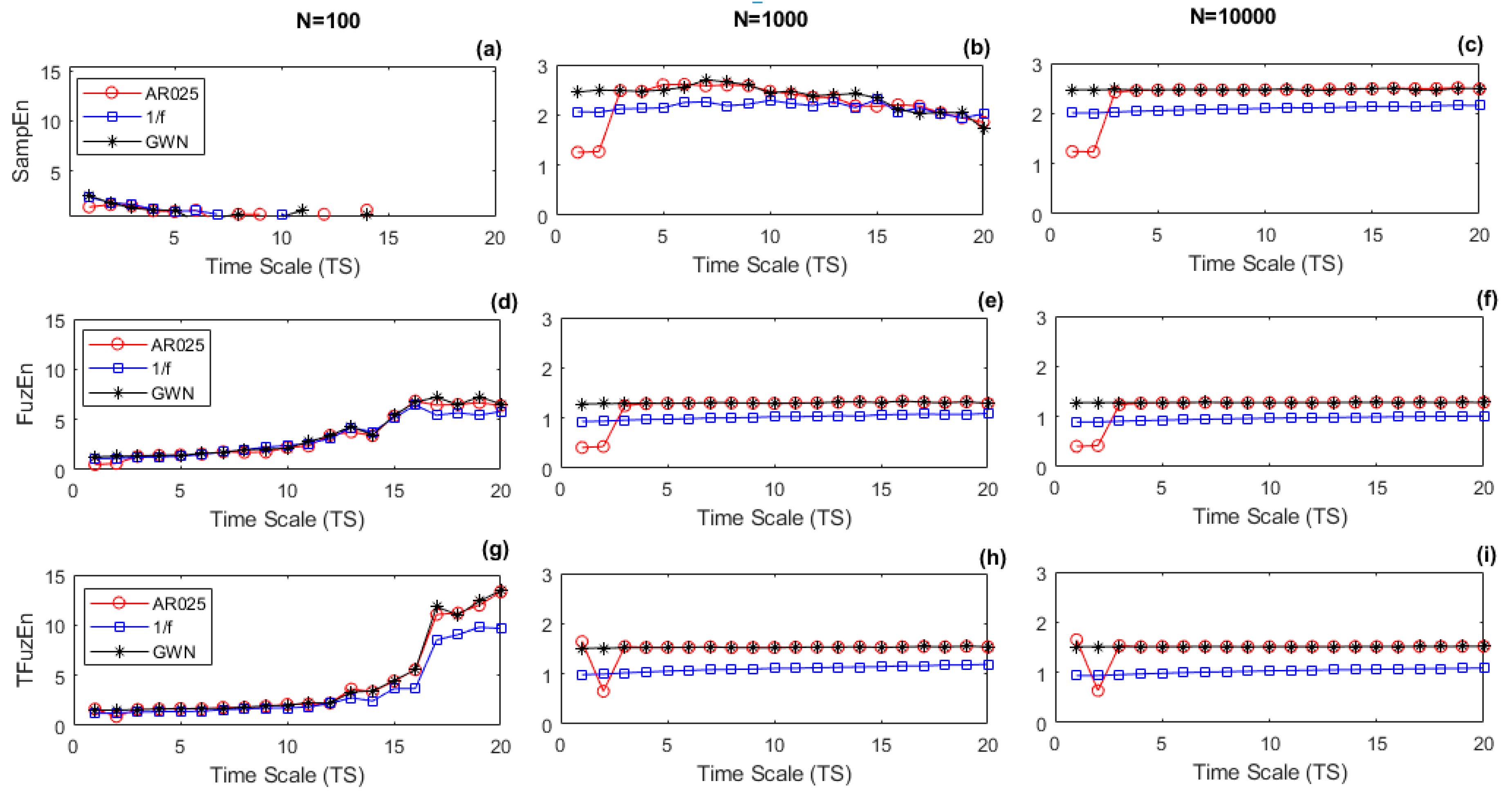
3.1. RMSE of Synthetic Time Series
- (a)
- at N = 10,000, FuzEn (Figure 1f), and IFuzEn (Figure 1l) had a similar behavior of SampEn (Figure 1c) for all the synthetic time series, but the courses of TFuzEn (Figure 1i) and ITFuzEn (Figure 1o) showed a different behavior for the AR025 series, particularly in TS = 1 where the entropy value was higher than TS = 2, presenting a kind of ripple.
- (b)
- at N = 1000, SampEn (Figure 1b) lost consistency in long scales (TS ≥ 10), which was evidenced specially in GWN and AR025 signals where the entropy value, that was higher than 1/f signal for N = 10,000, now was equal or lower that 1/f signal for N = 1000. On the contrary, all the fuzzy approaches (Figure 1e,h,k,n) showed a relative consistency for all the synthetic series at any time scale TS. TFuzEn (Figure 1h) and ITFuzEn (Figure 1n) continued showing a kind of ripple for the AR025 series between TS = 1 and TS = 2;
- (c)
- at N = 100, all the RMSE metrics lost consistency. Although SampEn values (Figure 1a) could not be obtained for time scales TS 7 (short series with less than 14 samples), all the fuzzy approaches could be computed for TS values between 1 and 20.
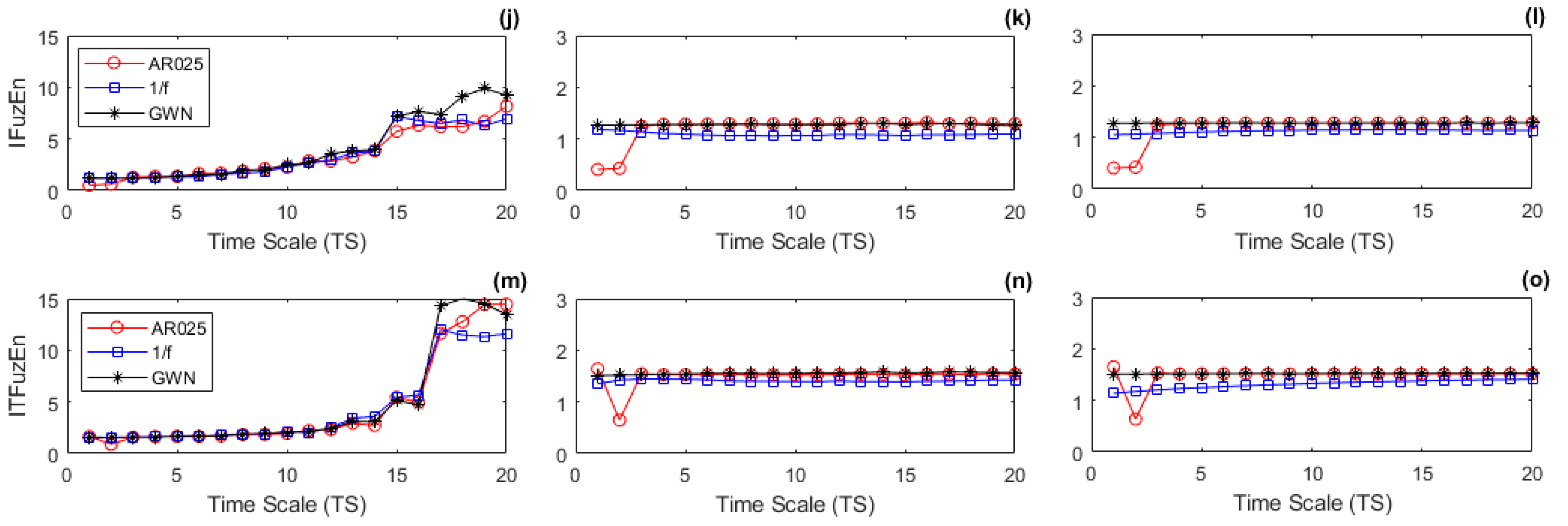
- (a)
- at N = 10,000: (i) although all the fuzzy approaches (Figure 2f,i,l,o,r) had a similar behavior of SampEn (Figure 2c) for the chaotic series (LM-3.7, LM-3.9, and HM signals), i.e., the courses exhibited an initial increase and then reached a plateau, the entropy values were lower and with smaller span than SampEn; (ii) only FuzEn (Figure 2f) had a similar behavior than SampEn in the totally predictable signal (LM-3.5); (iii) the course for LM-3.5 showed ripples in TFuzEn (Figure 2i), TRFuzEn (Figure 2l), IFuzEn (Figure 2o) and ITFuzEn (Figure 2r), being TRFuzEn the one with the most prominent ripple;
- (b)
- at N = 1000: (i) SampEn (Figure 2b) lost consistency in long scales (TS ≥ 10), which was evidenced specially in the LM-3.9 signal where the entropy value, that was higher or equal than the other signals for N = 10,000, now was lower than LM-3.7 and HM signals at long scales for N = 1000; (ii) all the fuzzy approaches (Figure 2e,h,k,n,q) showed a relative consistency for all the synthetic series at any time scale TS; (iii) only SampEn and FuzEn (Figure 2e) showed zero value for LM-3.5 in all the time scales; (iv) TFuzEn (Figure 2h), TRFuzEn (Figure 2k), IFuzEn (Figure 2n), and ITFuzEn (Figure 2q) continued showing a ripple in the course of LM-3.5;
- (c)
- at N = 100: (i) entropy values decreased in long time scales for SampEn (Figure 2a), while entropy values in fuzzy approaches tended to increase in long time scales; (ii) only SampEn and FuzEn (Figure 2d) showed a zero value for LM-3.5 in all the time scales; (iii) SampEn values could not be obtained for time scales TS 4 (short series with less than 25 samples) in LM-3.9 and for TS > 10 for the other series, but all the fuzzy approaches could be computed for all the TS values.
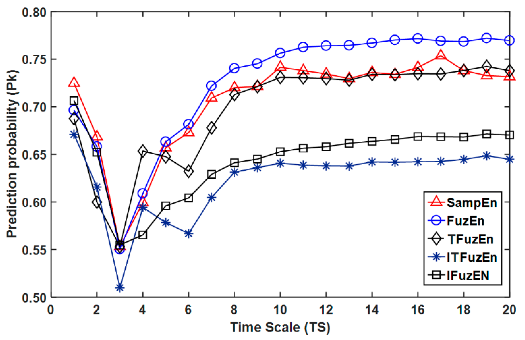
3.2. RMSE of EEG Signals
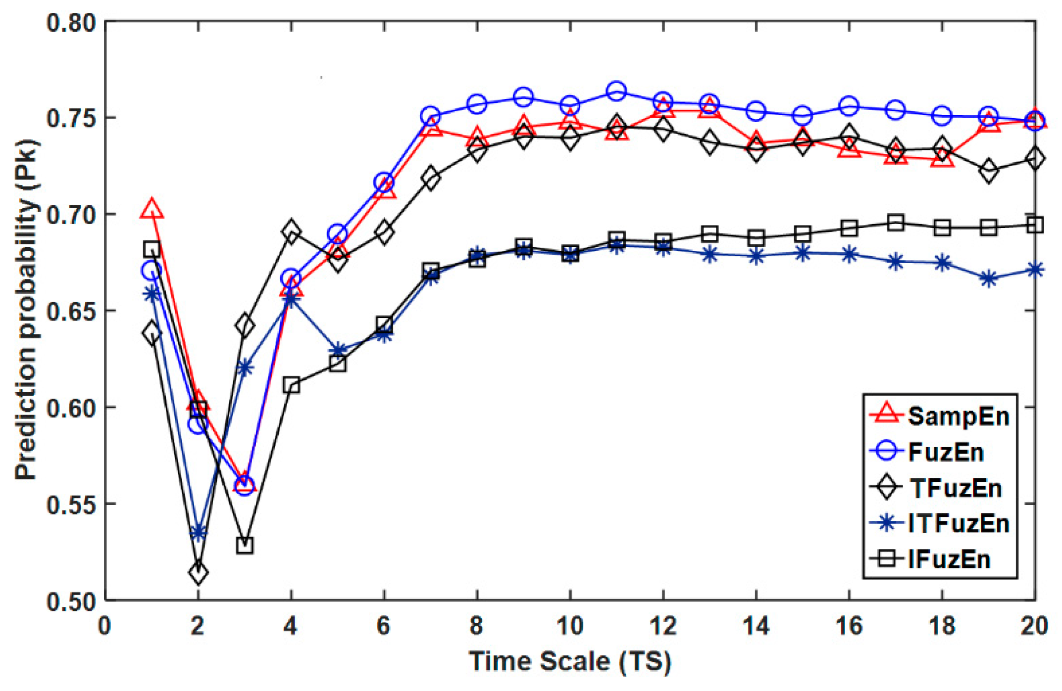
- (i)
- For long scales (6 ≤ TS ≤ 20), FuzEn, followed by SampEn, had the best Pk values, while ITFuzEn and IFuzEn had the worst performance.
- (ii)
- For short scale (TS = 1), the best Pk value was for SampEn, followed by IFuzEn and FuzEn. The lowest Pk values were obtained at TS = 3 for all the approaches in Figure 3 (2 ≤ RSS ≤ 5 vs. RSS = 6), while, for Figure 4 the lowest Pk were at TS = 2 for ITFuzEn, TFuzEn and TRFuzEn, and at TS = 3 for SampEn, FuzEn, and IFuzEn.
- (iii)
- When the Pk values were computed using FuzEn, the highest Pk values were obtained in time-scales larger than TS = 10. Since EEG signals were resampled to 128 Hz, time scales between TS = 10 and TS = 20 represent a EEG signal with frequency components that reduces the superior limit of the pass-band from 6.4 (TS = 10) to 3.2 Hz (TS = 20), gradually removing contributions in the (14–30 Hz), (8–14 Hz), and (4–8 Hz) bands of the EEG, and leaving the fluctuations in the (0.1–4 Hz) band of the EEG.
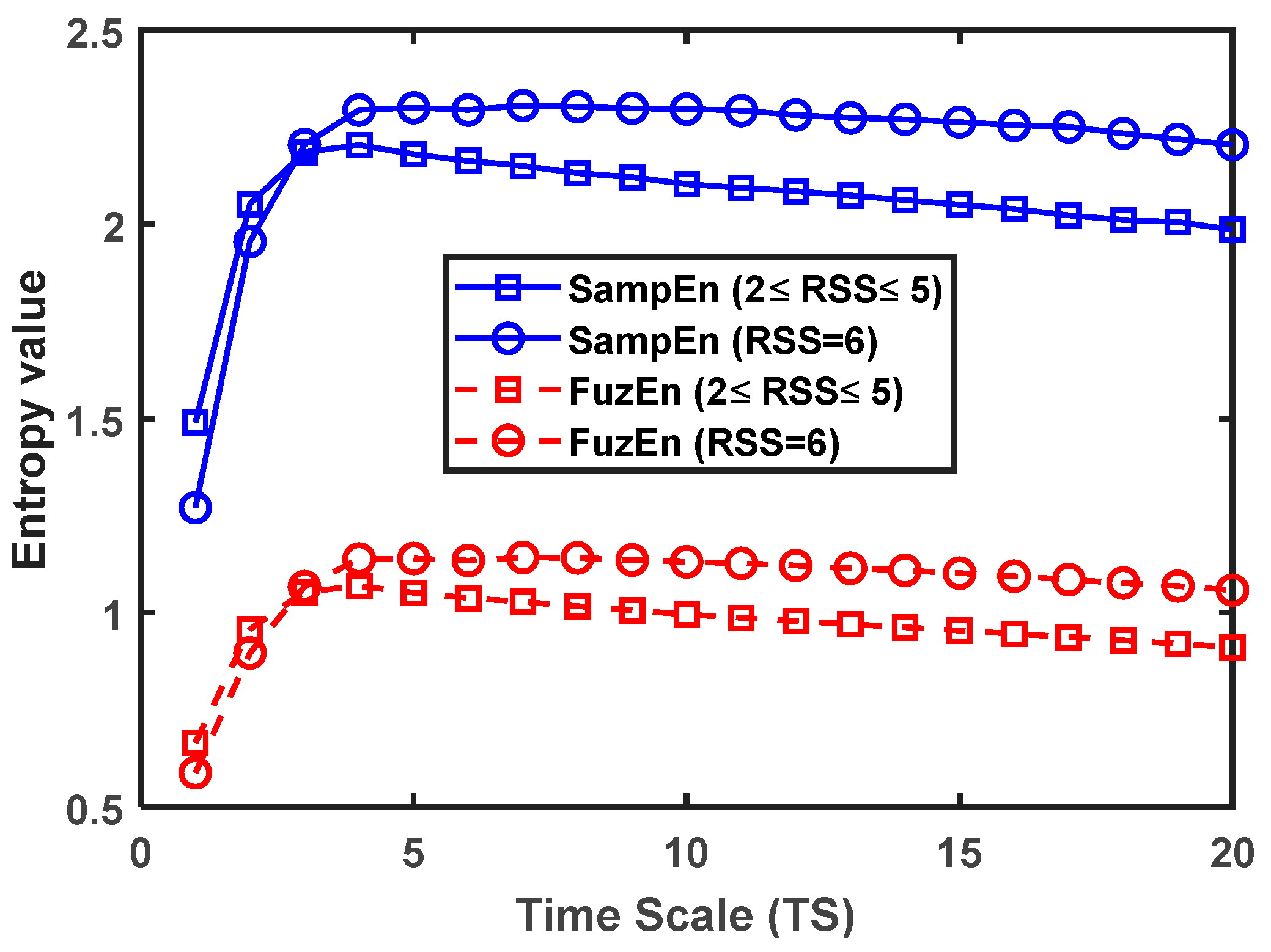
- (i)
- SampEn showed higher entropy values than FuzEn in all the scales for both groups (2 ≤ RSS ≤ 5 and RSS = 6).
- (ii)
- The courses of RMSE had a similar behavior in both metrics (SampEn and FuzEn) with an initial increase at short time scales (1 ≤ TS ≤ 3), a maximum near to TS = 4, and, then, a slow decrease at long time scales.
- (iii)
- In both metrics (SampEn and FuzEn), the entropy value was higher in responsive than in unresponsive state at short scales (1 ≤ TS ≤ 2), but this situation changed at longer scales (4 ≤ TS ≤ 20), i.e., the entropy value was lower in responsive than in unresponsive state.
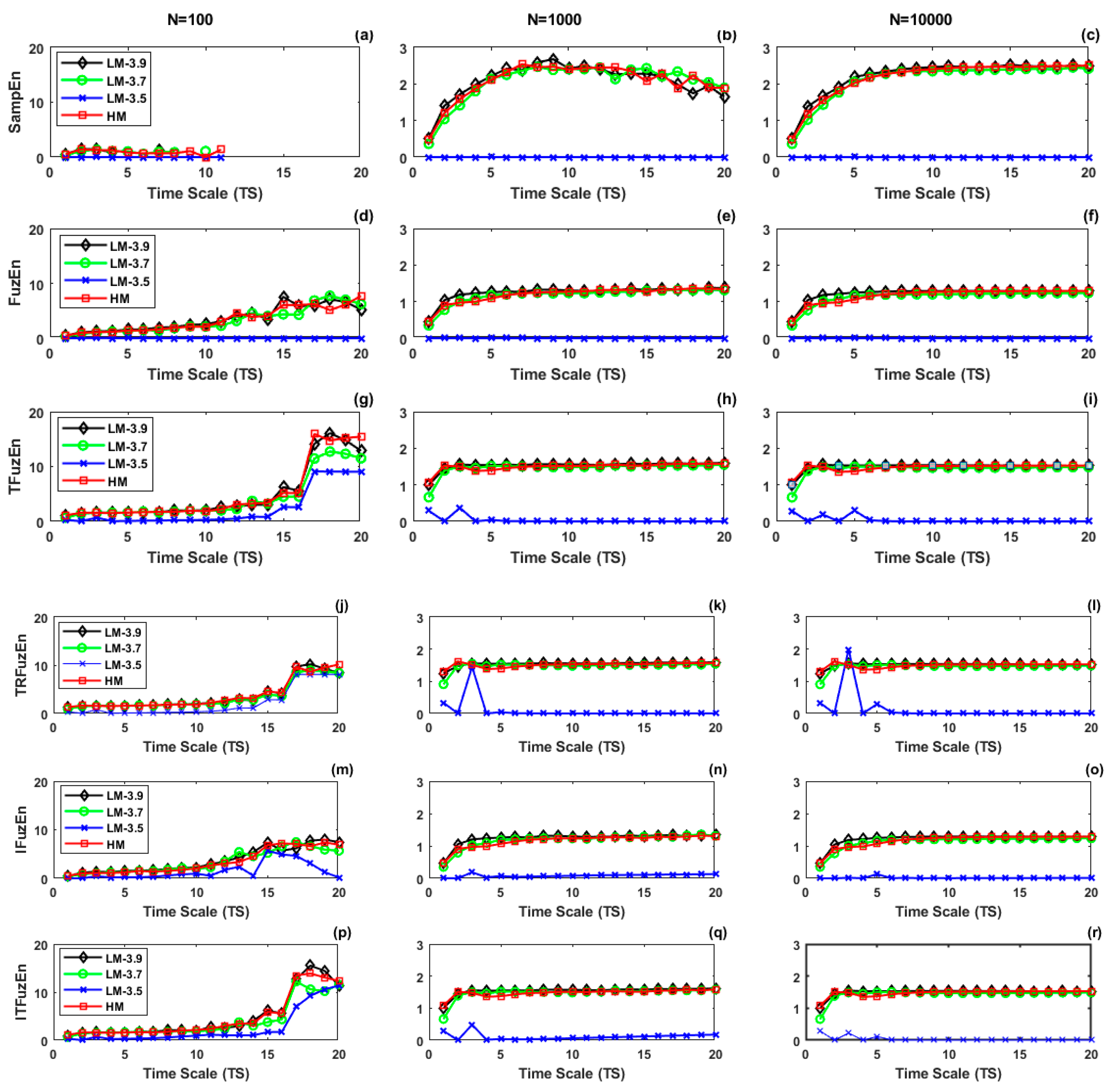
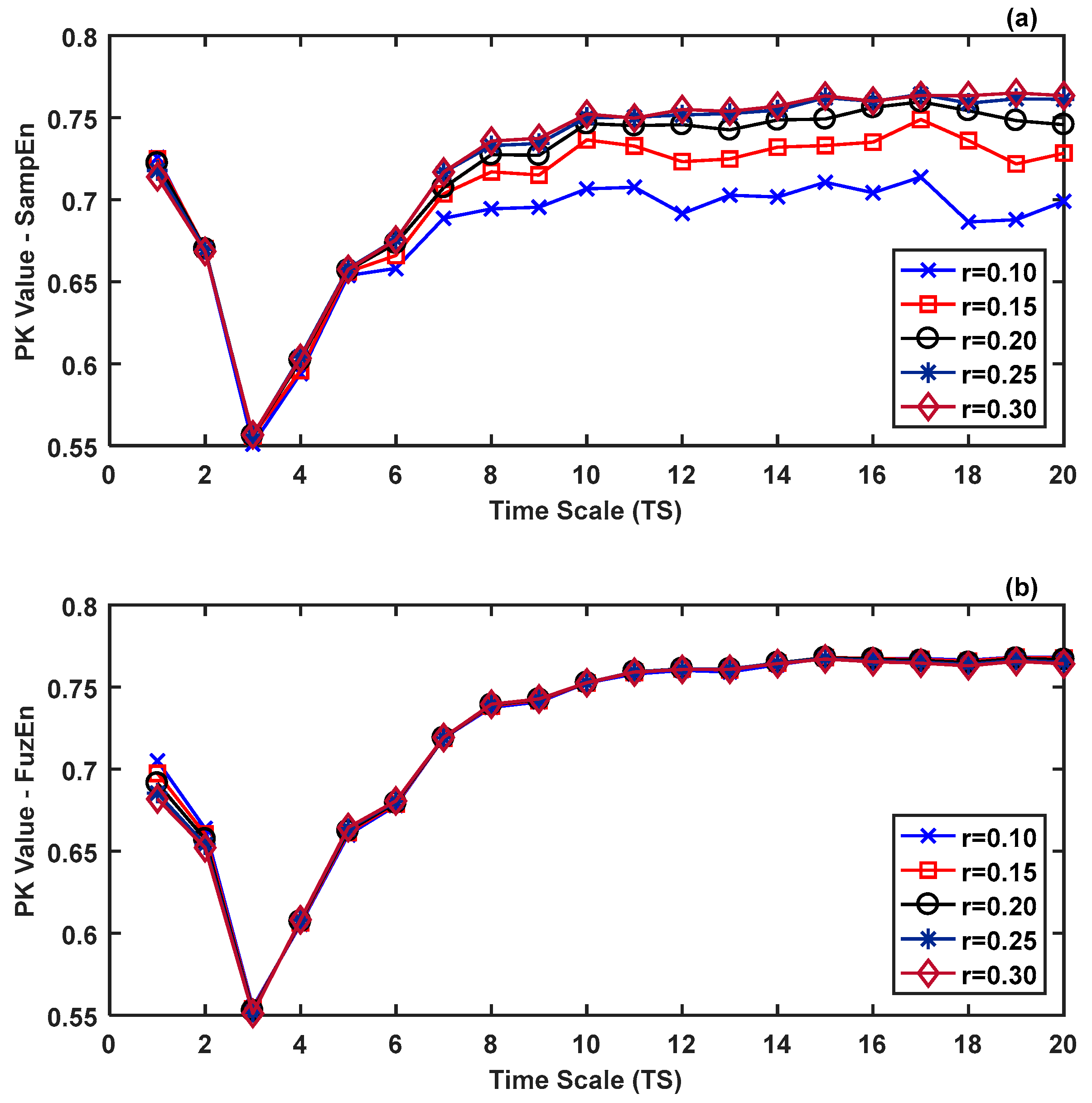
- (i)
- When SampEn was computed (Figure 6a), the Pk values were almost equal at short scales (1 ≤ TS ≤ 5) for all the values of the parameter r, but not for long scales.
- (ii)
- When FuzEn was computed (Figure 6b), the Pk values were practically equal for all the time scales TS and for all the values of the parameter r.
- (iii)
- The best Pk values were obtained for long scales in both RMSE using SampEn and using FuzEn.
4. Discussion
5. Conclusions
Author Contributions
Funding
Conflicts of Interest
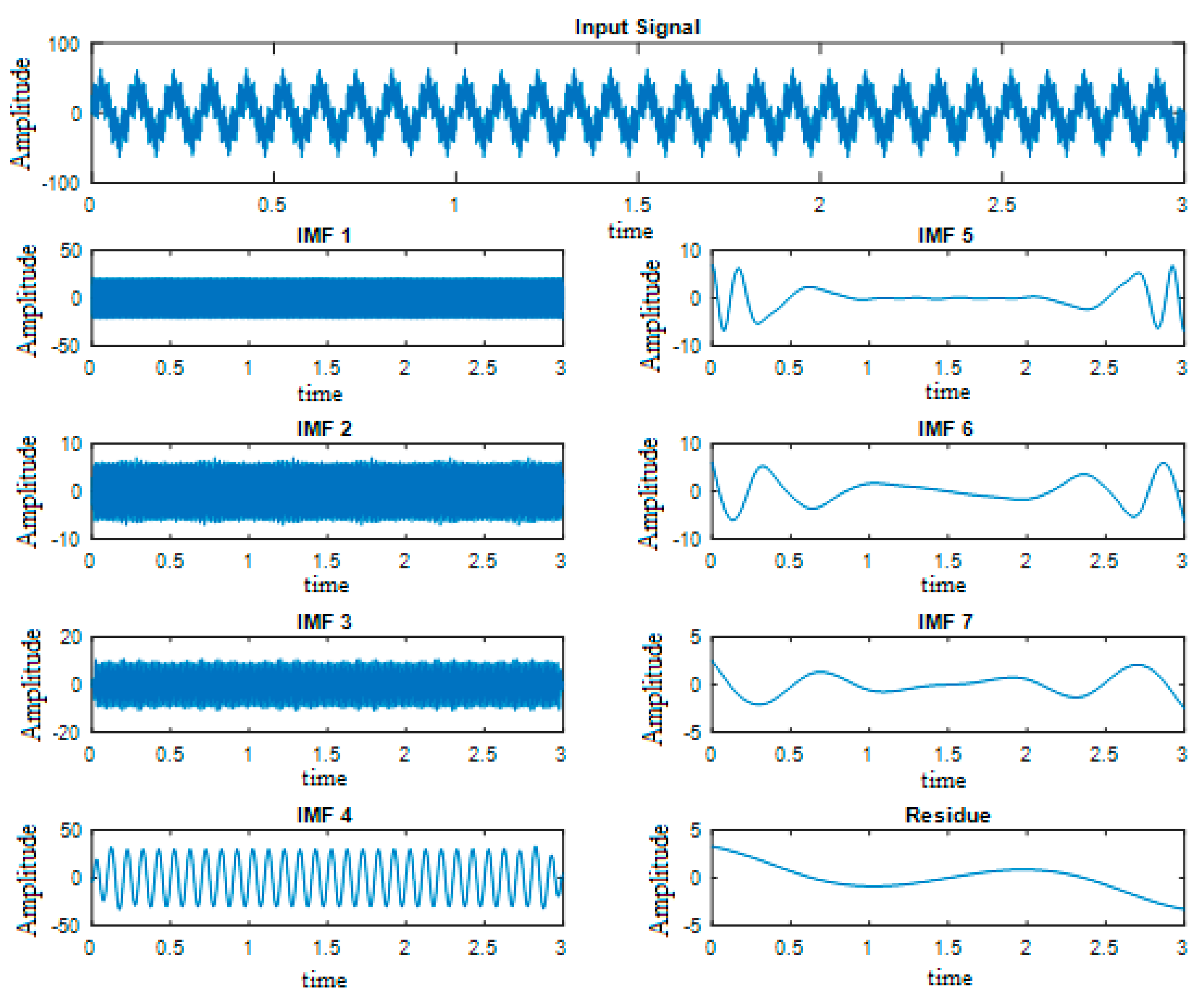
Appendix A. Empirical Mode Decomposition (EMD)
- (1)
- Identify all the local extrema of the signal (local minima and local maxima of ).
- (2)
- Interpolate between these local extrema, ending up with the upper and lower envelopes of ( and ). In this case a cubic spline interpolation was used according with work in [25].
- (3)
- Find the local trend as the average of the upper and lower envelopes, .
- (4)
- Determine the local fluctuation as, .
- (5)
- Evaluate as a candidate of inherent functions; will be an IMF if it satisfies two conditions: (i) the number of extrema and zero crossings must be either equal or differ at most by one; (ii) the average value between the envelope defined by the local maxima and the envelope defined by the local minima, must be zero at any point [23,25].
- (6)
- If is not an IMF, then go to step (1) with .
- (7)
- If is an IMF, save it as the intrinsic mode function , and calculate the residue Then, take , increment , and return to step (1).


References
- Chen, W.; Wang, Z.; Xie, H.; Yu, W. Characterization of surface EMG signal based on fuzzy entropy. IEEE Trans. Neural Syst. Rehabil. Eng. 2007, 15, 266–272. [Google Scholar] [CrossRef] [PubMed]
- Chen, W.; Zhuang, J.; Yu, W.; Wang, Z. Measuring complexity using FuzzyEn, ApEn, and SampEn. Med. Eng. Phys. 2009, 31, 61–68. [Google Scholar] [CrossRef] [PubMed]
- Zadeh, L.A. Fuzzy sets. Inf. Control 1965, 8, 338–353. [Google Scholar] [CrossRef] [Green Version]
- Xie, H.; Chen, W.; He, W.; Liu, H. Complexity analysis of the biomedical signal using fuzzy entropy measurement. Appl. Soft Comput. 2011, 11, 2871–2879. [Google Scholar] [CrossRef]
- Ji, L.; Li, P.; Li, K.; Wang, X.; Liu, C. Analysis of short-term heart rate and diastolic period variability using a refined fuzzy entropy method. Biomed. Eng. Online 2015, 14, 64. [Google Scholar] [CrossRef] [PubMed]
- Chen, C.; Jin, Y.; Lo, I.L.; Zhao, H.; Sun, B.; Zhao, Q.; Zheng, J.; Zhang, X.D. Complexity Change in Cardiovascular Disease. Int. J. Biol. Sci. 2017, 13, 1320–1328. [Google Scholar] [CrossRef]
- Xie, H.; Guo, T. Fuzzy entropy spectrum analysis for biomedical signals de-noising. In Proceedings of the 2018 IEEE International Conference on Biomedical & Health Informatics (BHI), Las Vegas, NV, USA, 4–7 March 2018; Volume 1, pp. 50–53. [Google Scholar]
- Ahmed, M.U.; Chanwimalueang, T.; Thayyil, S.; Mandic, D. A Multivariate Multiscale Fuzzy Entropy Algorithm with Application to Uterine EMG Complexity Analysis. Entropy 2017, 19, 2. [Google Scholar] [CrossRef]
- Girault, J.M.; Heurtier, A.H. Centered and Averaged Fuzzy Entropy to Improve Fuzzy Entropy Precision. Entropy 2018, 20, 287. [Google Scholar] [CrossRef]
- Cao, Z.; Lin, C.T. Inherent Fuzzy Entropy for the Improvement of EEG Complexity Evaluation. IEEE Trans. Fuzzy Syst. 2016, 26, 1032–1035. [Google Scholar] [CrossRef]
- Valencia, J.F.; Porta, A.; Vallverdú, M.; Claria, F.; Baranowski, R.; Orlowska, E.; Caminal, P. Refined multiscale entropy: Application to 24-h Holter recordings of heart period variability in healthy and aortic stenosis subjects. IEEE Trans. Biomed. Eng. 2009, 56, 2202–2213. [Google Scholar] [CrossRef]
- Valencia, J.F.; Vallverdú, M.; Porta, A.; Voss, A.; Schroeder, R.; Vázquez, R.; de Luma, A.B.; Caminal, P. Ischemic risk stratification by means of multivariate analysis of the heart rate variability. Physiol. Meas. 2013, 34, 325–338. [Google Scholar] [CrossRef]
- Bari, V.; Valencia, J.F.; Vallverdú, M.; Girardengo, G.; Marchi, A.; Bassani, T.; Caminal, P.; Cerutti, S.; George, A.L., Jr.; Brink, P.A.; et al. Multiscale complexity analysis of the cardiac control identifies asymptomatic and symptomatic patients in long QT syndrome type 1. PLoS ONE 2014, 9, e93808. [Google Scholar] [CrossRef] [PubMed]
- Bari, V.; Girardengo, G.; Marchi, A.; De Maria, B.; Brink, P.A.; Crotti, L.; Schwartz, P.J.; Porta, A. A Refined Multiscale Self-Entropy Approach for the Assessment of Cardiac Control Complexity: Application to Long QT Syndrome Type 1 Patients. Entropy 2015, 17, 7768–7785. [Google Scholar] [CrossRef] [Green Version]
- Valencia, J.F.; Melia, U.; Vallverdú, M.; Borrat, X.; Jospin, M.; Jensen, E.W.; Porta, A.; Gambús, P.L.; Caminal, P. Assessment of Nociceptive Responsiveness Levels during Sedation-Analgesia by Entropy Analysis of EEG. Entropy 2016, 18, 103. [Google Scholar] [CrossRef]
- Costa, M.; Goldberger, A.L.; Peng, C.K. Multiscale entropy analysis of biological signals. Phys. Rev. E 2005, 71, 021906. [Google Scholar] [CrossRef] [PubMed]
- Riihijarvi, J.; Wellens, M.; Mahonen, P. Measuring Complexity and Predictability in Networks with Multiscale Entropy Analysis. In Proceedings of the EEE INFOCOM 2009, Rio de Janeiro, Brazil, 19–25 April 2009; Volume 1, pp. 1107–1115. [Google Scholar]
- Wen, H. A Review of the Hénon Map and Its Physical Interpretations; School of physics, Georgia Institute of Technology: Atlanta, GA, USA, 2014. [Google Scholar]
- Ramsay, M.A.; Savege, T.M.; Simpson, B.R.; Goodwin, R. Controlled sedation with alphaxalone-alphadolone. Br. Med. J. 1974, 2, 656–659. [Google Scholar] [CrossRef] [PubMed]
- Melia, U.; Clariá, F.; Vallverdú, M.; Caminal, P. Filtering and thresholding the analytic signal envelope in order to improve peak and spike noise reduction in EEG signals. Med. Eng. Phys. 2014, 36, 547–553. [Google Scholar] [CrossRef] [Green Version]
- Richman, J.S.; Moorman, J.R. Physiological time-series analysis using approximate entropy and sample entropy. Am. J. Physiol. 2000, 278, H2039–H2049. [Google Scholar] [CrossRef] [Green Version]
- Pincus, S.M. Approximate entropy as a measure of system complexity. Proc. Natl. Acad. Sci. USA 1991, 88, 2297–2301. [Google Scholar] [CrossRef]
- Hu, K.; Ivanov, P.C.; Chen, Z.; Carpena, P.; Stanley, H.E. Effect of trends on detrended fluctuation analysis. Phys. Rev. E 2001, 64, 011114. [Google Scholar] [CrossRef] [Green Version]
- Huang, N.E.; Shen, Z.; Long, S.R.; Wu, M.C.; Shih, H.H.; Zheng, Q.; Yen, N.C.; Tung, C.C.; Liu, H.H. The empirical mode decomposition and the Hilbert spectrum for nonlinear and non-stationary time series analysis. Proc. R. Soc. Lond. Ser. A 1998, 454, 903–995. [Google Scholar] [CrossRef]
- Moghtaderi, A.; Flandrin, P.; Borgnat, P. Trend filtering via empirical mode decompositions. Comput. Stat. Data Anal. 2013, 58, 114–126. [Google Scholar] [CrossRef] [Green Version]
- Flandrin, P.; Rilling, G.; Gonçalves, P. Empirical mode decomposition as a filter bank. IEEE Signal Process. Lett. 2004, 11, 112–114. [Google Scholar] [CrossRef]
- Flandrin, P.; Gonçalves, P.; Rilling, G. Detrending and denoising with empirical mode decompositions. In Proceedings of the EUSIPCO 2004, Vienna, Austria, 6–10 September 2004; pp. 1581–1584. [Google Scholar]
- Rilling, G.; Flandrin, P.; Gonçalves, P. Empirical mode decomposition, fractional Gaussian noise, and Hurst exponent estimation. In Proceedings of the IEEE International Conference on Acoustics, Speech, and Signal Processing 2005, Philadelphia, PA, USA, 23–23 March 2005; pp. 489–492. [Google Scholar]
- Smith, W.D.; Dutton, R.; Smith, N.T. Measuring the performance of anesthetic depth indicators. Anesthesiology 1996, 84, 38–51. [Google Scholar] [CrossRef] [PubMed]


| Groups | Score | Description | No. EEG Windows |
|---|---|---|---|
| 2 ≤ RSS ≤ 5 | RSS = 2 | The patient is awake, quiet and cooperative | 422 |
| RSS = 3 | The patient is drowsy but responds to commands | 641 | |
| RSS = 4 | The patient is asleep with brisk response to stimulus | 428 | |
| RSS = 5 | The patient is asleep with sluggish response to stimulus | 360 | |
| RSS = 6 | No response (absence of movement) to firm nail-bed pressure. | 782 | |
| GAG = 0 | Absence of nausea reflex after endoscopy tube insertion | 411 | |
| GAG = 1 | Presence of nausea reflex after endoscopy tube insertion | 125 | |
© 2019 by the authors. Licensee MDPI, Basel, Switzerland. This article is an open access article distributed under the terms and conditions of the Creative Commons Attribution (CC BY) license (http://creativecommons.org/licenses/by/4.0/).
Share and Cite
Valencia, J.F.; Bolaños, J.D.; Vallverdú, M.; Jensen, E.W.; Porta, A.; Gambús, P.L. Refined Multiscale Entropy Using Fuzzy Metrics: Validation and Application to Nociception Assessment. Entropy 2019, 21, 706. https://doi.org/10.3390/e21070706
Valencia JF, Bolaños JD, Vallverdú M, Jensen EW, Porta A, Gambús PL. Refined Multiscale Entropy Using Fuzzy Metrics: Validation and Application to Nociception Assessment. Entropy. 2019; 21(7):706. https://doi.org/10.3390/e21070706
Chicago/Turabian StyleValencia, José F., Jose D. Bolaños, Montserrat Vallverdú, Erik W. Jensen, Alberto Porta, and Pedro L. Gambús. 2019. "Refined Multiscale Entropy Using Fuzzy Metrics: Validation and Application to Nociception Assessment" Entropy 21, no. 7: 706. https://doi.org/10.3390/e21070706