3.1. Time Evolution
The
q-voter model is based on the random sequential updating, which means that in an elementary update only one spin can change its state and thus one of three events is possible: the concentration of the positive opinion
increases or decreases by
or remains constant with the respective probabilities:
For our model on the infinite (
) complete graph:
Using probabilities given by Equation (
5) we can simulate trajectories of a random variable
, as done in [
3,
30]. However, we can also write the evolution equation of the corresponding expected value. For
we can safely assume, which is confirmed also by Monte Carlo simulations [
3] that random variable
localizes to the expected value:
where
, because one Monte Carlo step corresponds to
N elementary updates, i.e.,
.
Therefore for
we obtain the following rate equation:
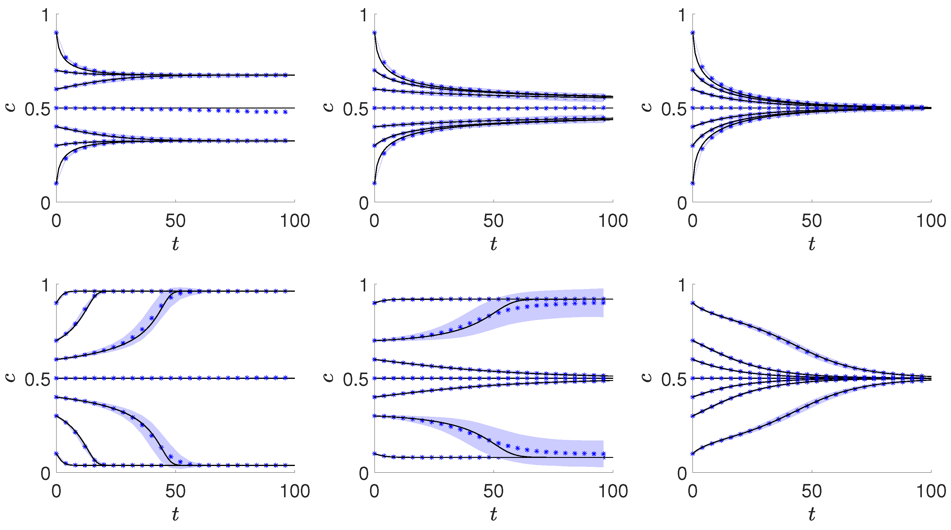
Sample trajectories obtained from Equation (
6) and independently from the Monte Carlo simulations for the systems of size
are shown in
Figure 1. It is seen that the agreement between the Monte Carlo and the analytical results is high, even for relatively small system, what is expected in case of a complete graph. Therefore, all other results will be presented based on the analytical calculations.
Preliminary results, presented in
Figure 1, suggest that there is a continuous phase transition for
and
(upper panels in
Figure 1), whereas a discontinuous one for
and
(bottom panels in
Figure 1). In the middle bottom panel metastability is visible, i.e., the final concentration of positive opinions depends on the initial state. In the metastable region a standard deviation is much larger for trajectories starting from
near the borders of basins of attraction. To explore deeper the possibility of the existence of discontinuous phase transitions within the model, we calculate the dependence between the stationary value of
, as a function of the probability of anticonformity
p.
3.2. Stationary States
To calculate stationary values of concentration
we must solve the following equation:
where
plays a role of an effective force [
30,
39]. One solution of the above equation, namely
, is straightforward because it is seen that for
the right side of quation (
7) equals to zero. The stability of this solution can be checked within linear stability analysis [
39]. The fixed point
is stable if [
39]:
From Equation (
5):
and thus, we obtain:
It means that
is a stable fixed point for
At
the fixed point
loses stability and for
it becomes unstable, which is also visible in
Figure 1.
Unfortunately, we are not able to calculate analytically other steady states, i.e., generally solve Equation (
8) in the form
for arbitrary values of
and
. However, following [
30] we can easily derive the opposite relation:
We use the above formula to plot
simply rotating the figure
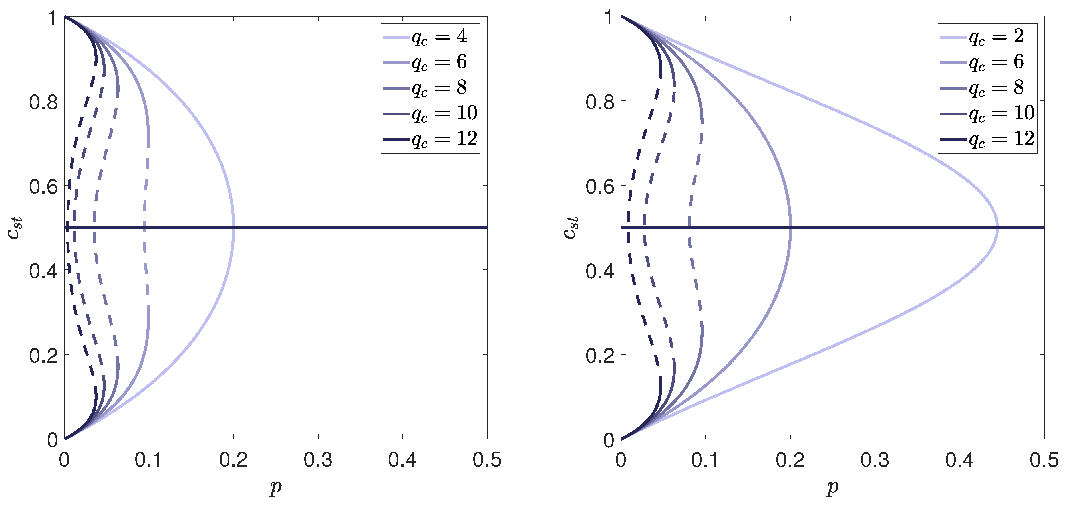
. Results for
and
are presented in
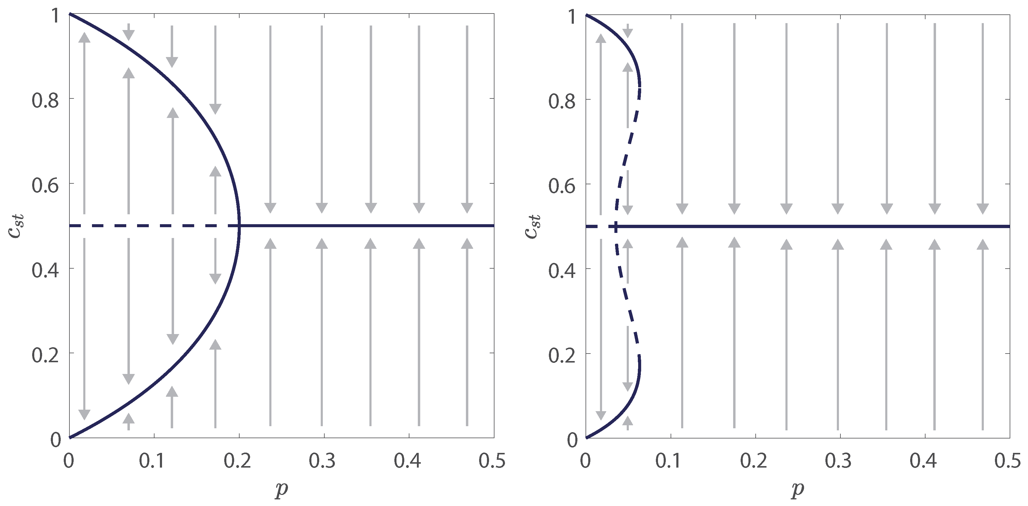
Figure 2 and
Figure 3. Although
Figure 2 shows only two examples (
and
), out of many presented in
Figure 3, it helps to better visualize what actually happens with the system. First of all, it is visible that there is a phase transition between phase with up-down (yes-no) symmetry and the phase in which this symmetry is broken, i.e., one of two opinions wins.
Moreover, it is seen that the phase transition is continuous for some values of parameters
and
, whereas for others it is discontinuous. For example, for the fixed value
the transition is continuous for
but for
it is discontinuous, see
Figure 3. Similarly, for the fixed value
the phase transition is continuous for
and
, whereas for
it is discontinuous. In case of a discontinuous phase transition, hysteresis is clearly seen, which means that the system can reach ordered or disordered state depending, on the initial conditions. The direction in which the system moves is indicated by the arrows in
Figure 2.
In case of a continuous phase transition function
has only one extremum—a maximum at
. The value
is the critical point, above which the stationary state has an up-down symmetry. It should be also noticed that in this case point
coincides with the bifurcation point
, given by Equation (
12), at which the fixed point
changes stability. From the perspective of nonlinear dynamics, point
is a point of the supercritical pitchfork bifurcation [
28,
39], see left panel in
Figure 2.
On the other hand, in case of a discontinuous phase transition function
has 3 extrema—a minimum at
and two maxima located symmetrically with respect to the line
at
and
. The value
is called the lower spinodal and
is called the upper spinodal. For
the system reaches a phase in which one of two opinions wins (
), independently of the initial state of the system. On the other hand, for
the system reaches a phase with up-down symmetry (
), independently of the initial state of the system. The most interesting is the metastable region which corresponds to
. In this region there is a phase coexistence and the stationary state depends on the initial one. In this case, the bifurcation point
, given by Equation (
12) coincides with the lower spinodal. From the perspective of nonlinear dynamics, point
is a point of the subcritical pitchfork bifurcation [
28,
39], see right panel in
Figure 2.
To derive the phase diagram, we need to calculate:
The lower spinodal as a function of parameters . It corresponds to the value of
at
, so it can be easily calculated from the relation
given by Equation (
13). In the case of a continuous phase transition this is simply the critical point
, which separates two phases. In this case, it corresponds to the maximum of
, whereas in case of a discontinuous phase transition it corresponds to the minimum of
, as seen in
Figure 2 and
Figure 3. As already written,
is also a pitchfork bifurcation point, given by Equation (
12), at which a steady state
changes stability, i.e., for
an agreement phase (
) is stable and disagreement phase (
) is unstable. This indicates that independently on the initial state of the system an agreement phase is reached. Although
has been already calculated within linear stability analysis, we will show that indeed it can be also obtained from Equation (
13).
The tricritical point, i.e., the value of as a function of for which the transition switches from continuous to discontinuous. As described above at this point the minimum at changes to maximum and thus this point can be also easily derived by calculating the point in which the second derivative of p changes the sign.
The upper spinodal as a function of parameters . As written above, in case of discontinuous phase transition
has two maxima at
and
and the value
is the upper spinodal, so it can be also derived from the relation
given by Equation (
13). In theory calculations are straightforward. Unfortunately, it occurs that finding an analytical formula for
for arbitrary values of parameters
and
is impossible and the upper spinodal will be obtained numerically.
The point of the phase transition . For a continuous phase transition, it is straightforward, as described above, because it corresponds to the value of at . In fact, for a continuous phase transition all three points: lower spinodal , upper spinodal and the point of the phase transition collapse to the single critical point, i.e., . For a discontinuous phase transition, it is far less trivial. The transition point is placed between lower and upper spinodals. In thermodynamics it corresponds to the point, at which phases are in the equilibrium, i.e., corresponding thermodynamic potential has minima of equal depth. Here we will also introduce an equivalent of a potential and use it to calculate the transition point.
As written above, the lower spinodal corresponds to the value of
p at
. However, for this value denominator in Equation (
13) equals zero and therefore we have to take the limit
and use L‘Hospital’s rule:
First of all, we see that indeed we obtained exactly the same result as within linear stability analysis, see Equation (
12). Moreover, it is seen that for
the results reduces to the formula for the original
q-voter model with anticonformity, derived in [
30]. On the other hand, if we put
and
we obtain:
whereas for the model with independence, introduced in [
30] the following result was obtained:
which is very close to the result for the
q-voter model with anticonformity for
and
. So, it seems that changing
for the fixed value of
or vice versa we can tune the model from the ‘anticonformity’ regime to the ‘independence’ regime, in which discontinuous phase transitions are possible. However, it should be stressed here that this result may be valid only in case of a complete graph, i.e., when we neglect all spatial correlations. In this case, both types of nonconformity, anticonformity and independence, tries to disorder the system. However, in general anticonformity should support active bonds, whereas independence introduces just random changes and thus we expect that on graphs with high clustering coefficient the difference between two types of nonconformity would be stronger. To check this prediction we plan to investigate the model on different graphs.
As written above, we can easily calculate the tricritical value
, for which transition changes from continuous to discontinuous, from the following condition:
To calculate the upper spinodal we should first find points at which
has maxima, but for this the following equation has be solved for
:
which is in general impossible within an analytical treatment. However, it can be easily done numerically.
Yet, it is less obvious how to calculate the point of the discontinuous phase transition. One natural possibility to solve the problem is to use the Landau approach, similarly as it was done in [
30]. We have to stress here that in [
30] only the lower spinodal was calculated within this approach. However, in general it could be used to derive analytical formulas also for the upper spinodal, the point of the phase transition, as well as the tricritical point. Before we proceed to apply the Landau approach, let us describe the method in an accessible way for researchers not trained in the theory of phase transitions.
3.3. Landau Approach for Continuous and Discontinuous Phase Transitions
Landau theory was originally proposed to describe continuous phase transitions [
38]. Landau introduced an order parameter, here the stationary value of
m given by Equation (
3), to distinguish between phases of the system:
in a disordered state (traditionally above the critical point), whereas
in an ordered phase (traditionally below the critical point). Additionally, Landau assumed that the thermodynamical potential, originally the Gibbs free energy, is not only a function of certain thermodynamical quantities, such as temperature and pressure, but it is also a function of an order parameter. In general, different potential could be used, for example a potential
as a function of the order parameter
m and the probability of nonconformity
p has been introduced for the
q-voter model in [
30] and here we will use the same approach. Finally, Landau assumed that the value of
m near the critical point is small and thus the potential can be expanded into a power series:
For a system with up-down symmetry,
, all odd terms must disappear and thus
. If we additionally ignore higher powers of
m we obtain:
The condition of the stable equilibrium is equivalent to the condition for a minimum of the potential and thus:
From the necessary condition for a minimum, i.e., the first condition of Equation (
21), we obtain two solutions:
(disordered phase) and
(ordered phase). Inserting these solutions into the condition of stability (sufficient condition for a minimum), i.e., the second condition of Equation (
21), we obtain:
which means that
A changes its sign during transition from one phase to another, i.e., the critical point corresponds to
. However, it should be noticed that the stability condition (
21) at the critical point (i.e., for
) gives:
Moreover, in order to obtain for
real values of
m corresponding to the ordered state, i.e.,
we also need
. Therefore,
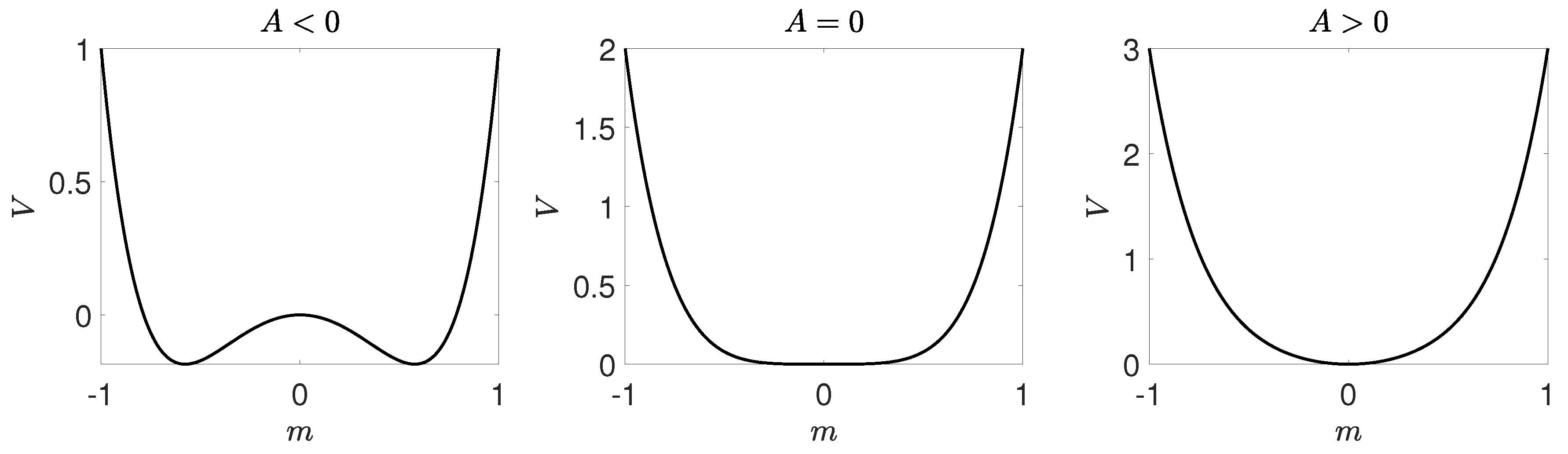
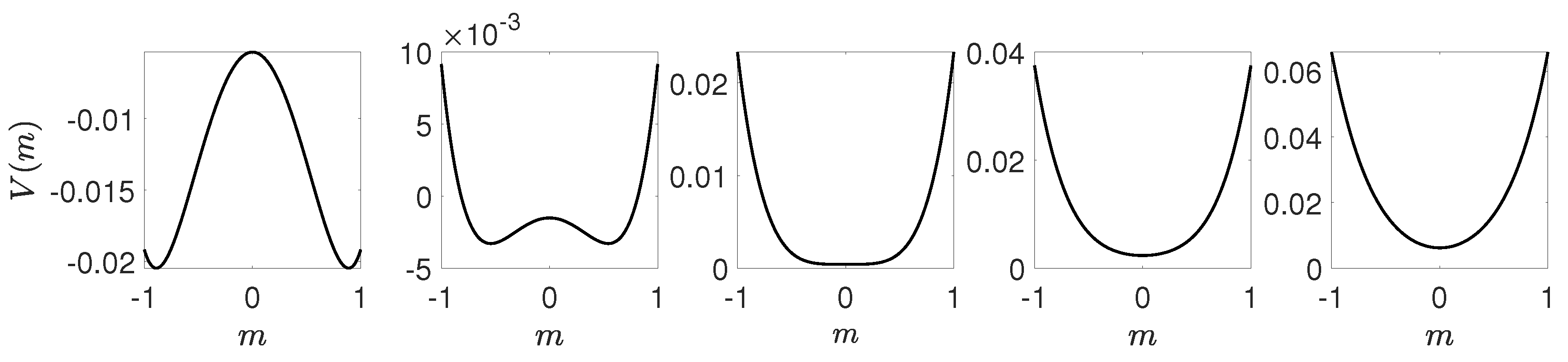
the Landau theory describes continuous phase transitions only for . In
Figure 4 we present a potential, given by Equation (
20), for
(specifically for
) and three values of
A:
,
and
. It is seen that indeed for
the potential has three extrema: maximum at
and two minima corresponding to
. For
the potential has only one extremum: minimum at
. This means that for
the steady state
loses stability. In the next section we will show that indeed this condition is equivalent with the condition given by Equation (
12).
Although originally Landau theory was introduced for continuous phase transitions, it occurs that
for we can describe discontinuous phase transitions [
40]. At the end of this section we will see why the assumption
is needed. For
we have to take into account the next term of the power series:
Again, we start with the condition for a stable equilibrium, i.e., minimum of the potential:
The necessary condition for a minimum, i.e., the first condition of Equation (
25) is fulfilled if:
Let us first check the stability of the first solution, which corresponds to the disordered phase. Inserting this solution into the condition of stability (sufficient condition for a minimum), i.e., the second condition of Equation (
25), we obtain:
which means that for
the solution
is stable, whereas for
it becomes unstable, analogously as in the case of continuous phase transition (i.e., for
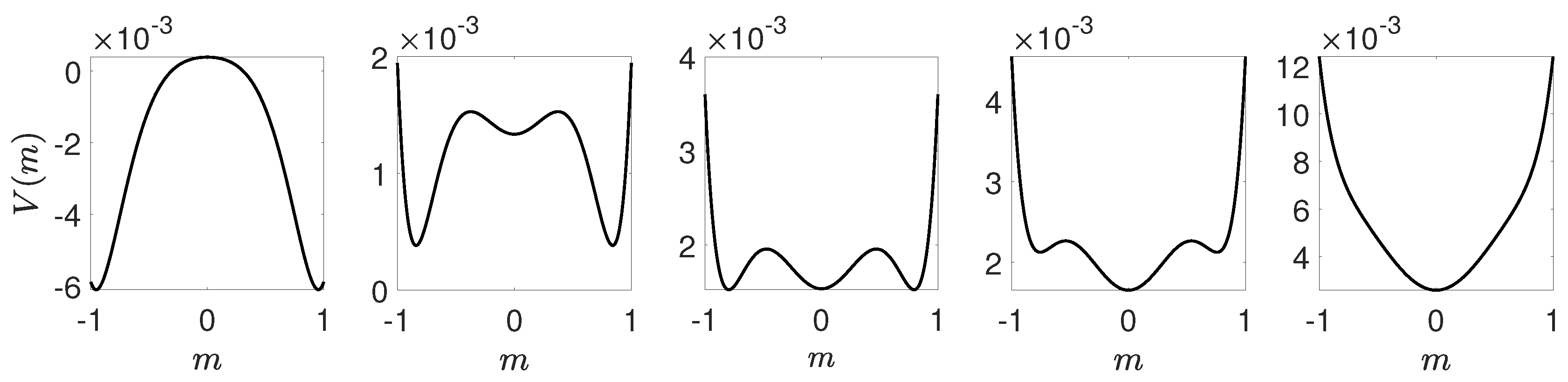
). However, the behavior of the potential is now very different, which is visible in
Figure 5.
It occurs that for a certain range of
, additionally to
, there are two other stable solutions given by the second condition in Equation (
26):
Because
m has to be a real number, for
and
we obtain:
if the following condition is fulfilled:
It means that for
two different types of phases (ordered and disordered) can coexist and region of metastability is limited by the spinodals:
Until now we have not yet calculated the point of the phase transition. For
the phase transition corresponds to the condition
, i.e., to the critical point, in which the solution
losses stability: for
the system always reaches one of two symmetrical ordered states (only these are stable) and for
the system always reaches disordered phase. For
the condition
still corresponds to the critical point, in which the solution
losses stability. However, for
the system can reach one of three different states, two ordered and one disordered, depending on the initial conditions. In thermodynamics the point of the phase transitions is defined as the point in which all phases are in the equilibrium, which is equivalent to the condition that potential
for the disordered phase is equal to the potential
of the ordered phases, where:
which leads to:
From the condition of equilibrium (
25) and from equality of potentials (
33) we obtain the set of equations:
Now we see why for
we had to assume that
. For
solutions would be complex. Inserting solution
, which corresponds to the jump of the order parameter at the transition point, to the condition (
33) we obtain that at the phase transition:
In
Figure 5 we see that indeed for this value of
A the potential has three minima of equal depth.
3.4. Application of the Landau Approach
To use this approach, we have to define an equivalent of a potential, which we called an effective potential [
30]:
It is worth mentioning that potentials, defined as above, are used also in nonlinear dynamics as an alternative way to visualize the dynamics of the first-order system [
39]. Within such an approach system always moves toward lower potential. Extrema of the potential (equilibrium states) correspond to fixed points: minima of
V correspond to stable fixed points and maxima correspond to unstable fixed points.
To use the classical Landau approach, we need to express the above potential in terms of the order parameter given by Equation (
3):
Now we expand the above potential into power series and keep only the first three terms of the expansion:
where:
We will use the results obtained within Landau approach, described in the previous section, which can be summarized as follows:
The critical point at which solution loses stability corresponds to .
For there is a tricritical point at , which means that for the transition is continuous, whereas for it is discontinuous.
For
the transition is continuous, see
Figure 6. In such a case potential takes one of two forms. For
potential
V is a double-well one with maximum at
(
). It means that the system always reaches one of two ordered phases: it is attracted by the minima of
V and repelled by the maximum at
, which corresponds to the unstable fixed point. For
the potential has only one minimum that corresponds to
(
). It means that a system always reaches disordered phase, i.e., the fixed point
(
) is stable.
For
the phase transition is discontinuous, see
Figure 7, and we can calculate the transition point
from the condition (
35) as well as spinodals
from (
31). As previously, the potential has two minima (ordered state) and one maximum (disordered state) for
, i.e., below lower spinodal. For
the potential has five extrema: two maxima corresponding to unstable fixed points and three minima corresponding to stable fixed points. Finally, for
the potential has only one minimum that corresponds to
(
).
We start with the critical point
at which solution
loses stability:
We see that within the Landau approach we have obtained exactly the same value as previously in Equation (
14). The transition is continuous as long as
and for
it is discontinuous, so we obtain the tricritical point from the condition:
Again, the Landau approach gives exactly the same value as obtained previously in Equation (
17). So far, we did not obtain any new result, but we have just shown that two approaches give exactly the same results, which is expected in case of a complete graph. However, at least theoretically, the Landau approach allows also to calculate upper spinodal, as well as the transition point for discontinuous phase transition. The upper spinodal can be calculated from the condition
, whereas the transition point from
, as long as
. Unfortunately, there are two problems: (1) analytical solution is difficult due to the form of coefficients
and
C and more importantly (2)
C becomes negative shortly after the tricritical point is reached and thus we are able to obtain results only for 3–4 values of
.
Therefore, we obtain the transition point numerically from the original form of the potential given by Equation (
37). In
Figure 6 and
Figure 7 potentials for
and
are shown respectively for several values of
p. In
Figure 6 we observe a typical behavior for a continuous phase transition, which mean that for
there are two symmetrical equally deep minima at
and
corresponding to two ordered phases: positive or negative opinion wins. With increasing
p minima are approaching each other and become shallower and finally for
they collapse to a single minimum at
. On the other hand, in
Figure 7 we observe a typical behavior for a discontinuous phase transition, which means that between the spinodals, i.e., for
there are 3 minima: two symmetrical
and
for the ordered phase and the third one at
corresponding to the disordered phase. At the transition point all three minima are equally deep and this allows us to calculate
for a discontinuous phase transition.
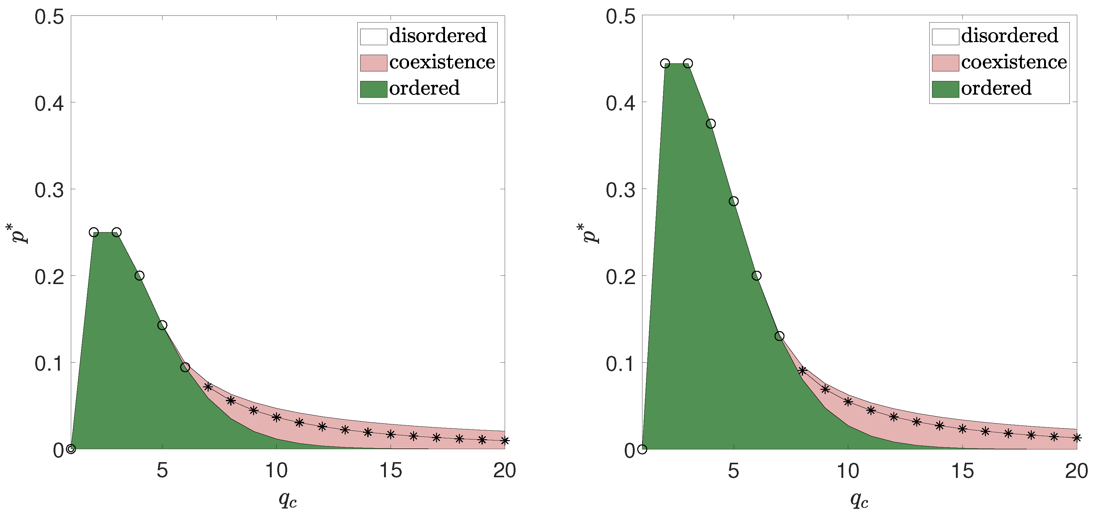
Collecting all results obtained above, we can draw the phase diagram. Examples of phase diagrams for two values of
are shown in
Figure 8. These diagrams remind the one for the
q-voter model with independence, presented in [
30]. In both cases the maximum value is obtained for
, which means that agreement is more likely when the size of the group needed for conformity is of size 2 or 3 and then decreases. Moreover, for
the transition becomes discontinuous. It means that hysteresis appears, i.e., there is an interval of width
between lower and upper spinodal in which the final state depends on the initial one and in which both phases (agreement and disagreement) coexist with each other. In this interval both phases are metastable: for
the agreement is more stable (represented by deeper minimum of the potential), whereas for
the disagreement is more stable.
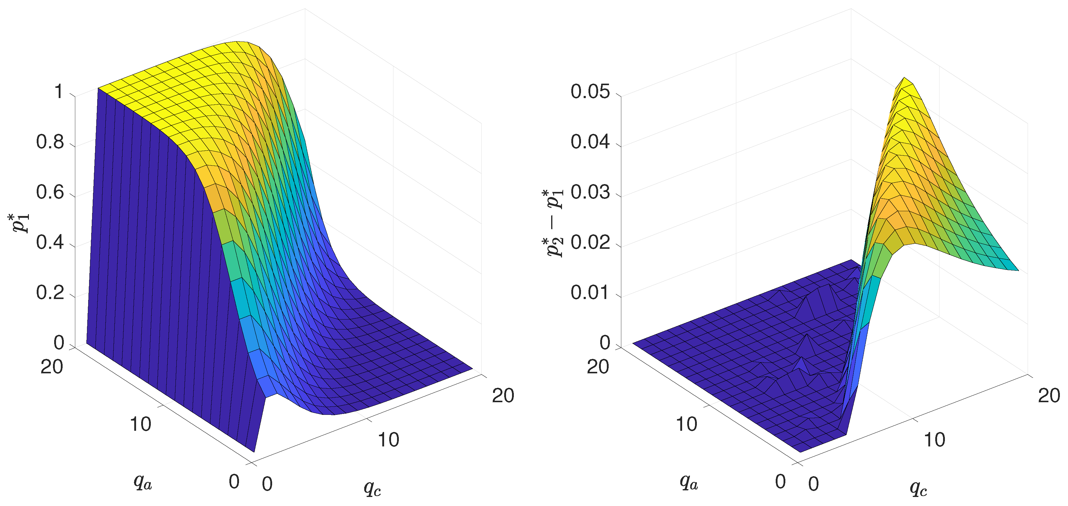
To illustrate results for all values of
and
we have decided to plot the lower spinodal line
(left panel in
Figure 9), as well as the width of hysteresis, which is defined as a distance between spinodals, (right panel in
Figure 9) as a function of both parameters
and
. In the left panel in
Figure 9 it is visible that for the fixed value of
the dependence between
and
is non-monotonic and for all
there is a maximum for
, which reminds the results for the
q-voter model with independence [
30]. On the other hand, for the fixed value of
the transition point
increases monotonically with
, which reminds the results for the
q-voter model with anticonformity [
30]. The width of hysteresis (right panel in
Figure 9) is increasing rapidly when the tricritical point is crossed, then reaches certain maximal value and then decreases again, which means that there are ‘optimal’ values of
and
for which the interval of metastability is the largest.


