A Novel Improved Feature Extraction Technique for Ship-Radiated Noise Based on IITD and MDE


Abstract
:1. Introduction
2. Theory of IITD-MDE
2.1. IITD Algorithm
2.1.1. ITD
2.1.2. Comparison of Baseline-Fitting Method
2.1.3. Intrinsic Scale Component (ISC)
2.1.4. IITD
2.2. MDE Algorithm
2.2.1. DE
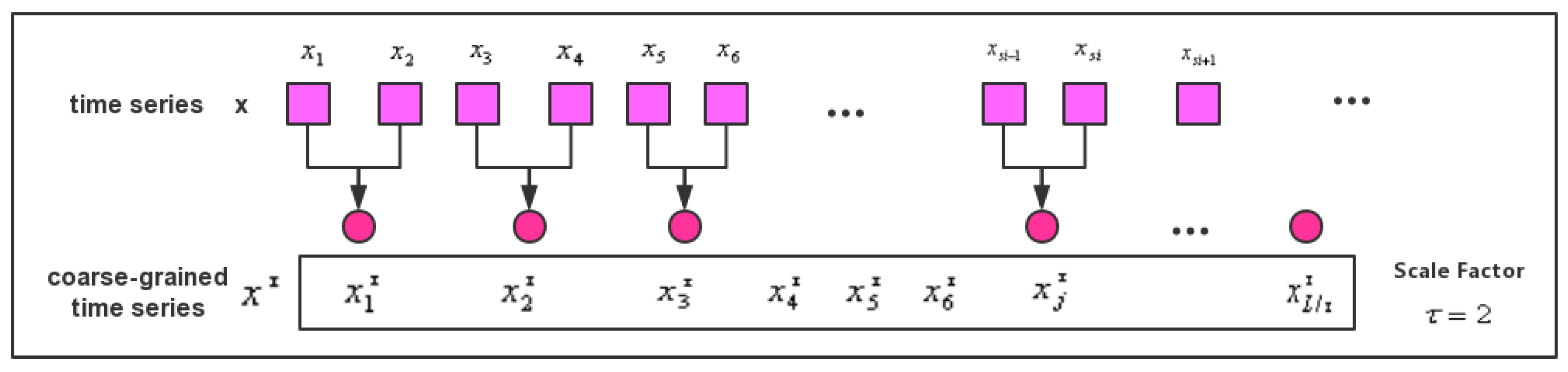
2.2.2. MDE
2.3. Comparison between ITD, IITD, and EMD
2.4. Comparison between MSE, MPE, and MDE
3. The Proposed Feature Extraction Method
- (1)
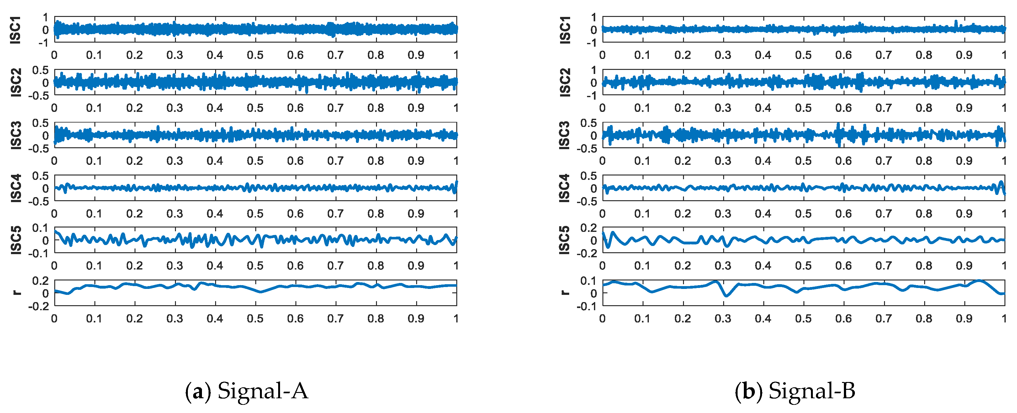
- Perform IITD on the five types of ship-radiated noise signals of the training data and decompose signals into a series of ISCs and one monotonic trend component.
- (2)
- Calculate the correlation between ISCs and the original signal, then select the ISCs with large correlation coefficients as the feature parameter.
- (3)
- Calculate their MDE value of the chosen ISCs and set scale factor to 20.
- (4)
- Input feature vectors to SVM to establish the classifier.
- (5)
- For the test dataset, extract their features using steps (1–3), then input the features into classifier for classification and get recognition rates.
4. Experimental Verification and Analysis
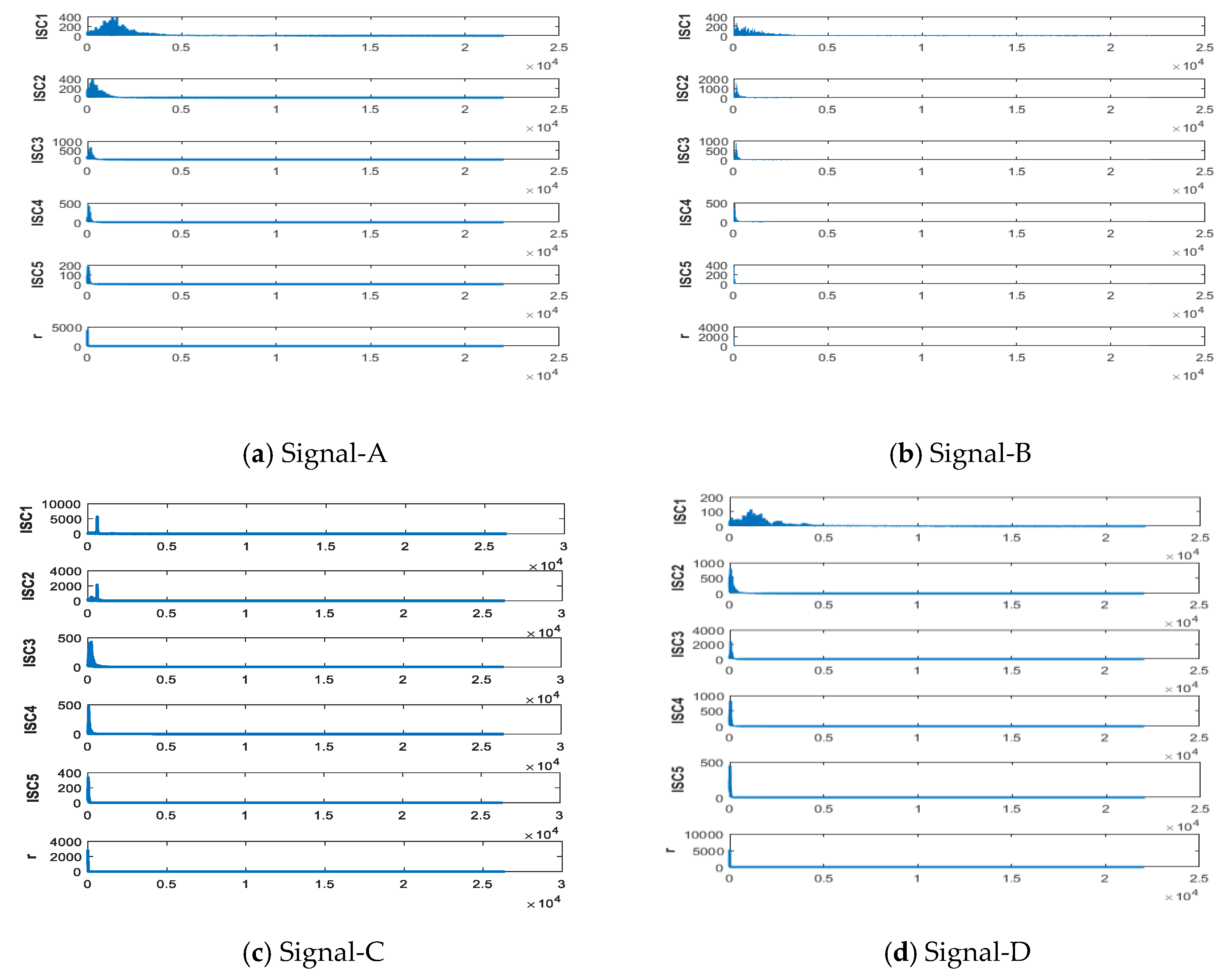
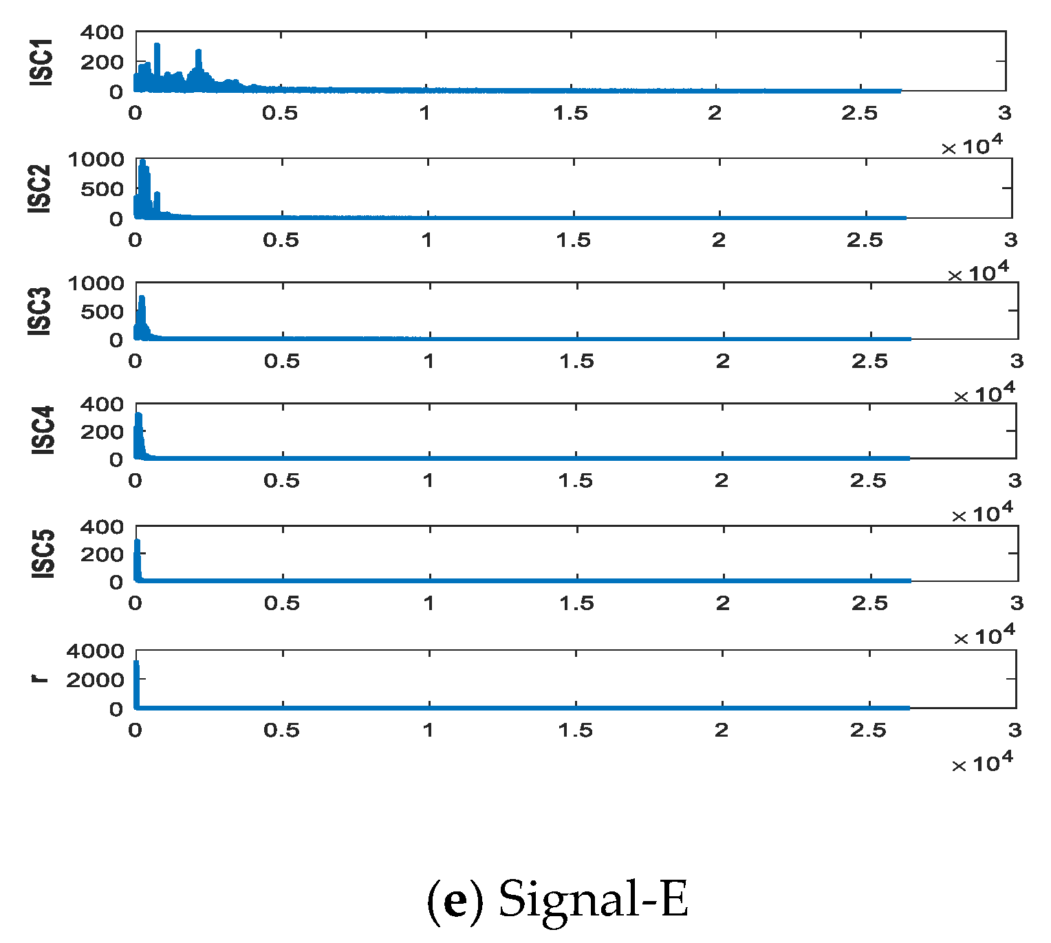
4.1. IITD Decomposition
4.2. ISC Choosen
4.3. Feature Extraction
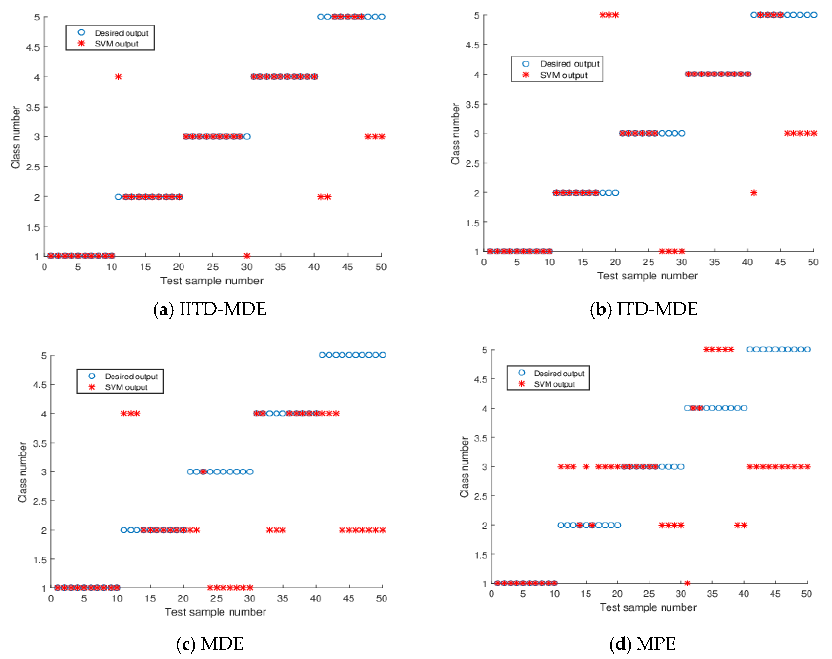
4.4. Ship Classification
5. Conclusions
Author Contributions
Funding
Conflicts of Interest
References
- Wang, S.; Zeng, X. Robust underwater noise targets classification using auditory inspired time-frequency analysis. Appl. Acoust. 2014, 78, 68–76. [Google Scholar] [CrossRef]
- Tucker, J.D.; Azimi-Sadjadi, M.R. Coherence-based underwater target detection from multiple disparate sonar platforms. IEEE J. Ocean. Eng. 2011, 36, 37–51. [Google Scholar] [CrossRef]
- Yan, Z.; Li, Y. Application of principal component analysis to ship-radiated noise classification and recogniion. Appl. Acoust. 2009, 28, 20–26. [Google Scholar]
- Zhang, X.H.; Wang, J.C.; Lin, L.J. Feature extraction of ship-radiated noises based on wavelet transform. Acta Acust. 1997, 22, 139–144. [Google Scholar]
- Huang, N.E.; Shen, Z.; Long, S.R.; Wu, M.C.; Shih, H.H.; Zheng, Q.; Yen, N.-C.; Tung, C.C.; Liu, H.H. The empirical mode decomposition and the Hilbert spectrum for nonlinear and non-stationary time series analysis. Proc. R. Soc. A Math. Phys. Eng. Sci. 1998, 454, 903–995. [Google Scholar] [CrossRef]
- Wu, Z.; Huang, N.E. A study of the characteristics of white noise using the empirical mode decomposition method. Proc. R. Soc. A: Math. Phys. Eng. Sci. 2004, 460, 1597–1611. [Google Scholar] [CrossRef]
- Restrepo, J.M.; Venkataramani, S.; Comeau, D.; Flaschka, H. Defining a trend for time series using the intrinsic time-scale decomposition. New J. Phys. 2015, 16, 085004. [Google Scholar] [CrossRef]
- Li, Z.; Li, Y.; Zhang, K. A Feature Extraction Method of Ship-Radiated Noise Based on Fluctuation-Based Dispersion Entropy and Intrinsic Time-Scale Decomposition. Entropy 2019, 21, 693. [Google Scholar] [CrossRef] [Green Version]
- Si, L.; Wang, Z.; Tan, C.; Liu, X. Vibration-Based Signal Analysis for Shearer Cutting Status Recognition Based on Local Mean Decomposition and Fuzzy C-Means Clustering. Appl. Sci. 2017, 7, 164. [Google Scholar] [CrossRef] [Green Version]
- Gao, Y.; Villecco, F.; Li, M.; Song, W. Multi-Scale Permutation Entropy Based on Improved LMD and HMM for Rolling Bearing Diagnosis. Entropy 2017, 19, 176. [Google Scholar] [CrossRef] [Green Version]
- Wu, Z.; Huang, N.E. Ensemble empirical mode decomposition: A noise assisted data analysis method Center for Ocean land Atmosphere Studies. Tech. Rep. 2006, 1, 1–41. [Google Scholar]
- Yeh, J.R.; Shieh, J.S.; Huang, N.E. Complementary ensemble empirical mode decomposition: A novel noise enhanced data analysis method. Adv. Adapt. Data Anal. 2010, 2, 135–156. [Google Scholar] [CrossRef]
- Li, Y.; Li, Y.; Chen, X.; Yu, J. Feature extraction of ship-radiated noise based on VMD and center frequency. J. Vib. Shock 2018, 37, 213–218. [Google Scholar]
- Li, Y.; Chen, X.; Yu, J.; Yang, X. A Fusion Frequency Feature Extraction Method for Underwater Acoustic Signal Based on Variational Mode Decomposition, Duffing Chaotic Oscillator and a Kind of Permutation Entropy. Electronics 2019, 8, 61. [Google Scholar] [CrossRef] [Green Version]
- Yang, H.; Li, Y.; Li, G. Energy analysis of ship-radiated noise based on ensemble empirical mode decomposition. J. Vib. Shock 2015, 34, 55–59. [Google Scholar]
- Li, Y.; Chen, X.; Yu, J. A Hybrid Energy Feature Extraction Approach for Ship-Radiated Noise Based on CEEMDAN Combined with Energy Difference and Energy Entropy. Processes 2019, 7, 69. [Google Scholar] [CrossRef] [Green Version]
- Frei, M.G.; Osorio, I. Intrinsic time-scale decomposition: Time–frequency–energy analysis and real-time filtering of non-stationary signals. Proc. R. Soc. A Math. Phys. Eng. Sci. 2007, 463, 321–342. [Google Scholar] [CrossRef]
- Chen, J.-S.; Wang, J.; Gui, L. An improved EEMD method and its application in rolling bearing fault diagnosis. J. Vib. Shock 2018, 37, 51–56. [Google Scholar]
- Feng, Z.; Lin, X.; Zuo, M.J. Joint amplitude and frequency demodulation analysis based on intrinsic time-scale decomposition for planetary gearbox fault diagnosis. Mech. Syst. Signal Process. 2016, 72, 223–240. [Google Scholar] [CrossRef]
- Martis, R.J.; Acharya, U.R.; Tan, J.H.; Petznick, A.; Tong, L.; Chua, C.K.; Ng, E.Y.K. Application of intrinsic time-scale decomposition (ITD) to EEG signals for automated seizure prediction signals for automated seizure prediction. Int. J. Neural Syst. 2013, 23, 1350023. [Google Scholar] [CrossRef]
- Bernardini, M.; Fredianelli, L.; Fidecaro, F.; Gagliardi, P.; Nastasi, M.; Licitra, G. Noise Assessment of Small Vessels for Action Planning in Canal Cities. Environments 2019, 6, 31. [Google Scholar] [CrossRef] [Green Version]
- Wang, D.-J.; Liu, Z.-W.; Wei, J.; Wang, W.; Nie, Z.-S. Method to correct atmospheric pressure effects based on ensemble empirical mode decomposition. Chin. J. Geophys. 2018, 61, 504–520. [Google Scholar]
- Gao, Y.-C. A Research on Application of Hilbert-Huang Transform in the Underwater Acoustic Signal Processing. Ph.D. Thesis, Harbin Engineering University, Harbin, China, 2009. [Google Scholar]
- Badino, A.; Borelli, D.; Gaggero, T.; Rizzuto, E.; Schenone, C. Airborne noise emissions from ships: Experimental characterization of the source and propagation over land. Appl. Acoust. 2016, 104, 158–171. [Google Scholar] [CrossRef]
- Bica, A.M.; Degeratu, M.; Demian, L.; Paul, E. Optimal Alternative to the Akima’s Method of Smooth Interpolation Applied in Diabetology. Surv. Math. Its Appl. 2006, 1, 41–49. [Google Scholar]
- De Araujo, D.B.; Tedeschi, W.; Santos, A.C.D.; Elias, J., Jr.; Neves, U.P.D.C.; Baffa, O. Shannon entropy applied to the analysis of event-related fMRI time series. NeuroImage 2003, 20, 311–317. [Google Scholar] [CrossRef]
- Zhao, Z.H.; Yang, S.P. Sample Entropy Based Roller Bearing Fault Diagnosis Method. J. Vib. Shock 2012, 31, 136–140. [Google Scholar]
- Li, W.; Shen, X.; Li, Y. A Comparative Study of Multiscale Sample Entropy and Hierarchical Entropy and Its Application in Feature Extraction for Ship-Radiated Noise. Entropy 2019, 21, 793. [Google Scholar] [CrossRef] [Green Version]
- Li, Y.; Wang, L.; Li, X.; Yang, X. A Novel Linear Spectrum Frequency Feature Extraction Technique for Warship Radio Noise Based on Complete Ensemble Empirical Mode Decomposition with Adaptive Noise, Duffing Chaotic Oscillator, and Weighted-Permutation Entropy. Entropy 2019, 21, 507. [Google Scholar] [CrossRef] [Green Version]
- Monge, J.; Gómez, C.; Poza, J.; Fernández, A.; Quintero, J. & Hornero, R. MEG analysis of neural dynamics in attention-deficit/hyperactivity disorder with fuzzy entropy. Med. Eng. Phys. 2015, 37, 416–423. [Google Scholar]
- Rostaghi, M.; Azami, H. Dispersion Entropy: A Measure for Time Series Analysis. IEEE Signal Process. Lett. 2016, 23, 610–614. [Google Scholar] [CrossRef]
- Costa, M.; Goldberger, A.L.; Peng, C.K. Multiscale entropy analysis of biological signals. Phys. Rev. E 2005, 71, 021906. [Google Scholar] [CrossRef] [PubMed] [Green Version]
- Azami, H.; Escudero, J. Coarse-Graining Approaches in Univariate Multiscale Sample and Dispersion Entropy. Entropy 2018, 20, 138. [Google Scholar] [CrossRef] [Green Version]
- Dagher, I.; Azar, F. Improving the SVM gender classification accuracy using clustering and incremental learning. Expert Syst. 2019, 36. [Google Scholar] [CrossRef]


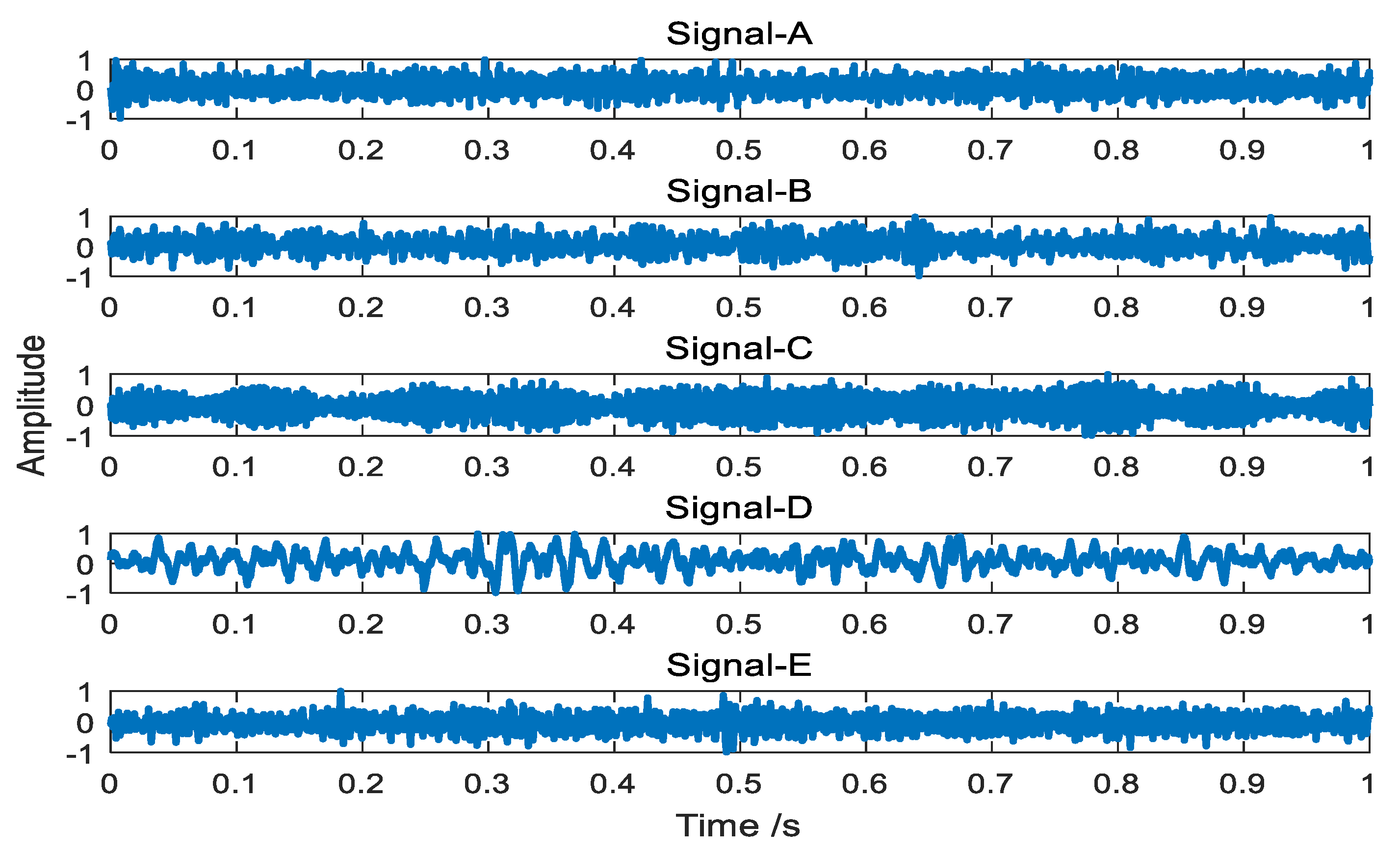
| Ship Signal | Signal-A | Signal-B | Signal-C | Signal-D | Signal-E |
| Feature Parameter | ISC2 | ISC4 | ISC2 | ISC4 | ISC3 |
| Methods | Accuracy Rate | ||
|---|---|---|---|
| Accuracy | Mean Squared Error | Squared Correlation Coefficient | |
| IITD-MDE | 86% | 0.56 | 0.7356 |
| ITD-MDE | 74% | 1.44 | 0.4661 |
| MDE | 50% | 2.32 | 0.2680 |
| MPE | 40% | 1.84 | 0.2386 |
© 2019 by the authors. Licensee MDPI, Basel, Switzerland. This article is an open access article distributed under the terms and conditions of the Creative Commons Attribution (CC BY) license (http://creativecommons.org/licenses/by/4.0/).
Share and Cite
Li, Z.; Li, Y.; Zhang, K.; Guo, J. A Novel Improved Feature Extraction Technique for Ship-Radiated Noise Based on IITD and MDE. Entropy 2019, 21, 1215. https://doi.org/10.3390/e21121215
Li Z, Li Y, Zhang K, Guo J. A Novel Improved Feature Extraction Technique for Ship-Radiated Noise Based on IITD and MDE. Entropy. 2019; 21(12):1215. https://doi.org/10.3390/e21121215
Chicago/Turabian StyleLi, Zhaoxi, Yaan Li, Kai Zhang, and Jianli Guo. 2019. "A Novel Improved Feature Extraction Technique for Ship-Radiated Noise Based on IITD and MDE" Entropy 21, no. 12: 1215. https://doi.org/10.3390/e21121215