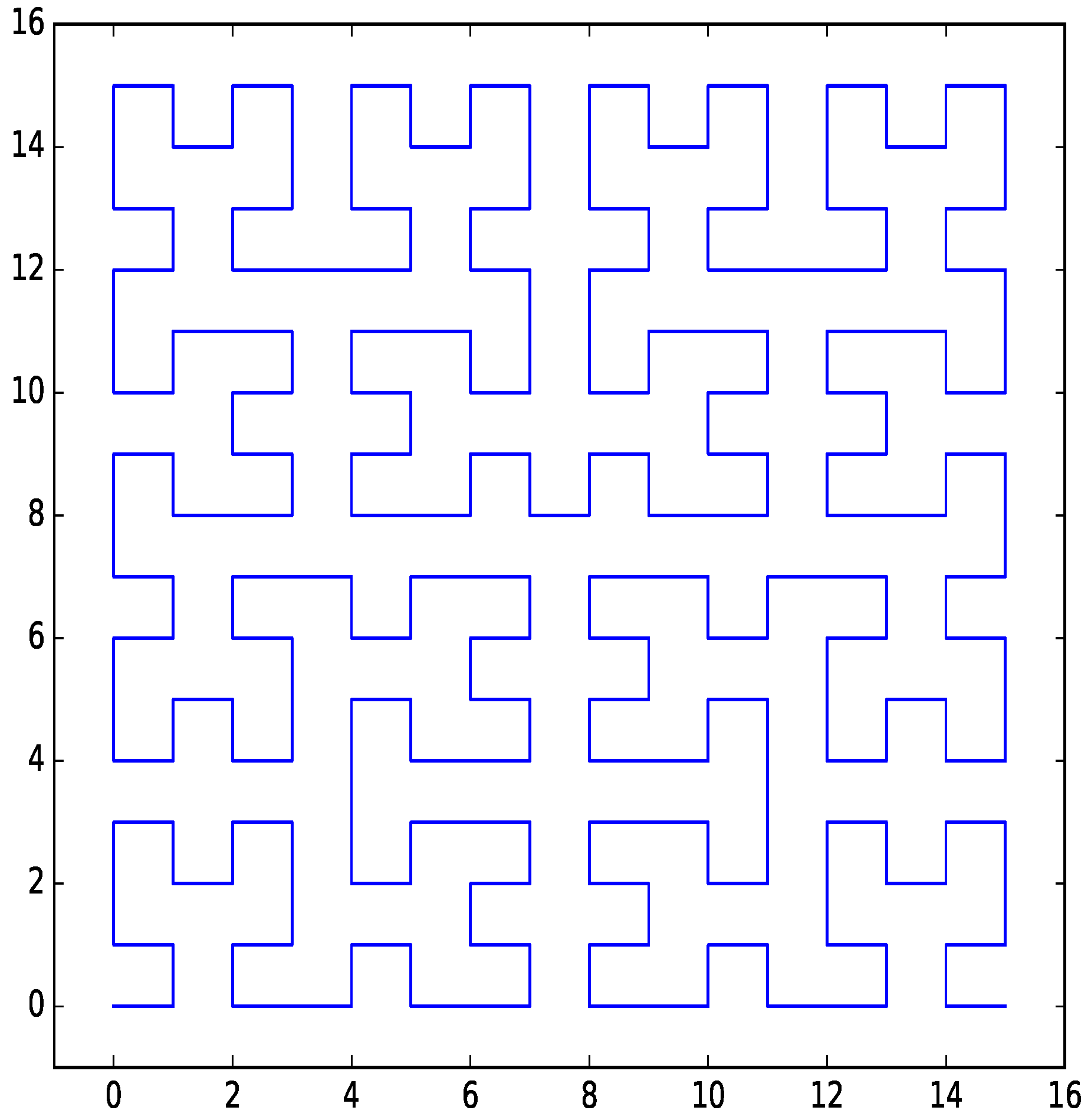
Figure 1.
Hilbert curve for two dimensions with four bits per dimension.
Figure 1.
Hilbert curve for two dimensions with four bits per dimension.
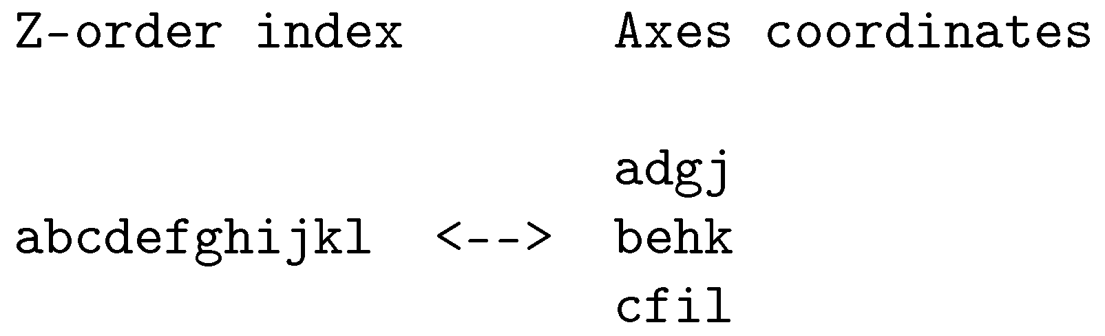
Figure 2.
Example of Z-order bit-interleaving for three dimensions with four bits per dimension.
Figure 2.
Example of Z-order bit-interleaving for three dimensions with four bits per dimension.
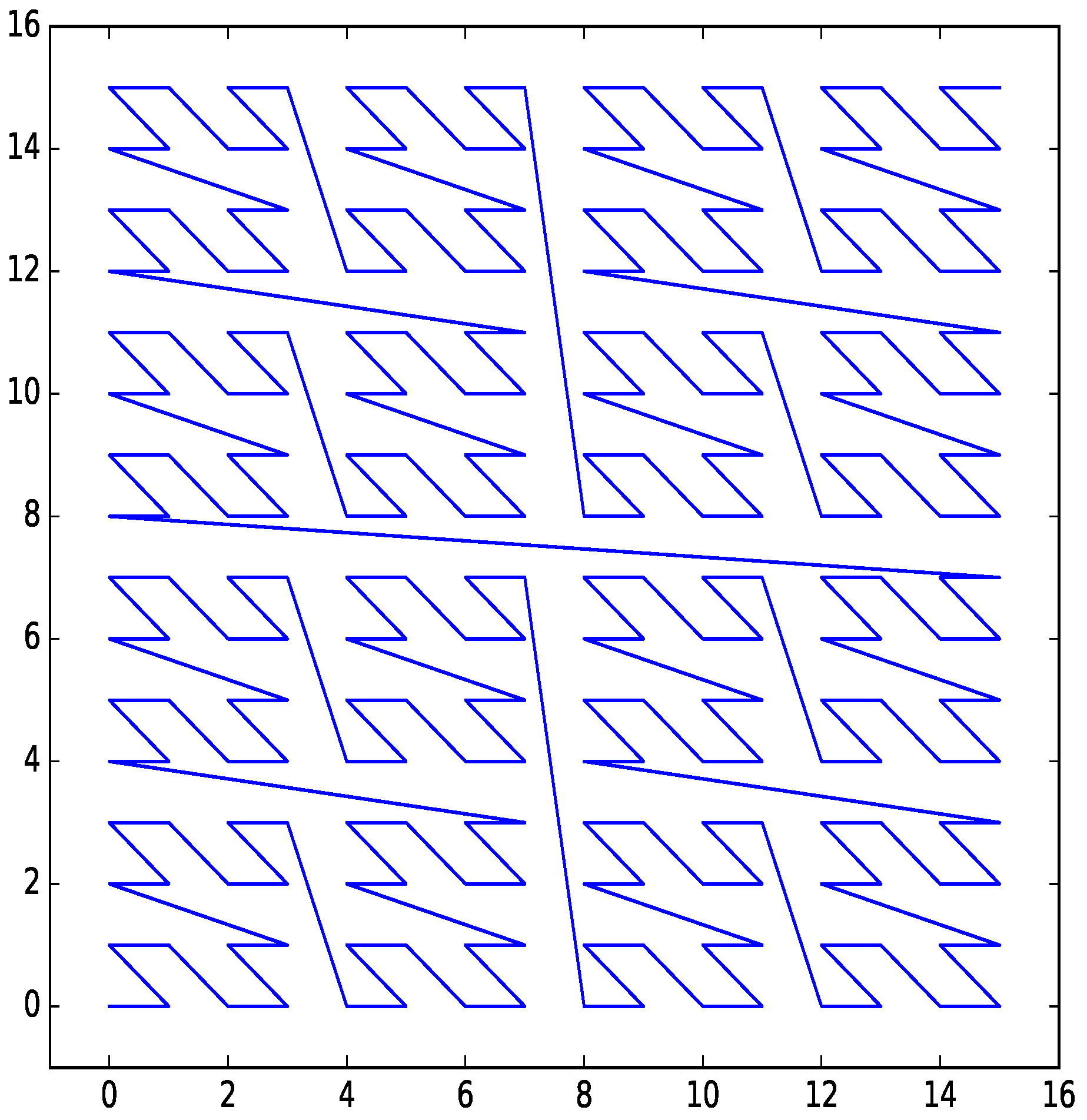
Figure 3.
Z-order curve for two dimensions with four bits per dimension.
Figure 3.
Z-order curve for two dimensions with four bits per dimension.
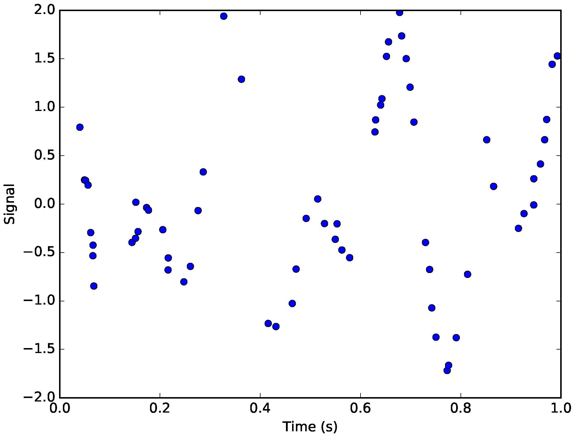
Figure 4.
The simulated signal. The points represent the non-uniformly sampled points from the original signal corrupted by Gaussian noise.
Figure 4.
The simulated signal. The points represent the non-uniformly sampled points from the original signal corrupted by Gaussian noise.
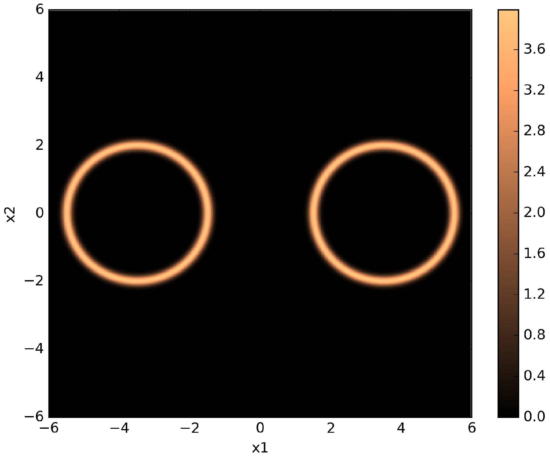
Figure 5.
Pseudo-color plot of a two-dimensional twin Gaussian shell with , , , and . The color values correspond to likelihood values.
Figure 5.
Pseudo-color plot of a two-dimensional twin Gaussian shell with , , , and . The color values correspond to likelihood values.
Figure 6.
Box-plot of log-evidence for the egg-crate problem for each TI method. TI-Stan with W=xx is denoted by ti stan, xx; TI-BSS-H with W=xx is denoted by tih, xx; and TI-BSS-Z with W=xx is denoted by tiz, xx.
Figure 6.
Box-plot of log-evidence for the egg-crate problem for each TI method. TI-Stan with W=xx is denoted by ti stan, xx; TI-BSS-H with W=xx is denoted by tih, xx; and TI-BSS-Z with W=xx is denoted by tiz, xx.
Figure 7.
Box-plot of run time in seconds for the egg-crate problem for each TI method. TI-Stan with W=xx is denoted by ti stan, xx; TI-BSS-H with W=xx is denoted by tih, xx; and TI-BSS-Z with W=xx is denoted by tiz, xx.
Figure 7.
Box-plot of run time in seconds for the egg-crate problem for each TI method. TI-Stan with W=xx is denoted by ti stan, xx; TI-BSS-H with W=xx is denoted by tih, xx; and TI-BSS-Z with W=xx is denoted by tiz, xx.
Figure 8.
Box-plot of log-evidence for the 10-D twin Gaussian shell problem for TI-Stan and TI-BSS-H. TI-Stan with W=xx is denoted by ti stan, xx and TI-BSS-H with W=xx is denoted by tih, xx.
Figure 8.
Box-plot of log-evidence for the 10-D twin Gaussian shell problem for TI-Stan and TI-BSS-H. TI-Stan with W=xx is denoted by ti stan, xx and TI-BSS-H with W=xx is denoted by tih, xx.
Figure 9.
Box-plot of run time in seconds for the 10-D twin Gaussian shell problem for TI-Stan and TI-BSS-H. TI-Stan with W=xx is denoted by ti stan, xx and TI-BSS-H with W=xx is denoted by tih, xx.
Figure 9.
Box-plot of run time in seconds for the 10-D twin Gaussian shell problem for TI-Stan and TI-BSS-H. TI-Stan with W=xx is denoted by ti stan, xx and TI-BSS-H with W=xx is denoted by tih, xx.
Figure 10.
Box-plot of log-evidence for the 30-D twin Gaussian shell problem for TI-Stan.
Figure 10.
Box-plot of log-evidence for the 30-D twin Gaussian shell problem for TI-Stan.
Figure 11.
Box-plot of run time in seconds for the 30-D twin Gaussian shell problem for TI-Stan.
Figure 11.
Box-plot of run time in seconds for the 30-D twin Gaussian shell problem for TI-Stan.
Figure 12.
Box-plot of log-evidence for the 100-D twin Gaussian shell problem for TI-Stan.
Figure 12.
Box-plot of log-evidence for the 100-D twin Gaussian shell problem for TI-Stan.
Figure 13.
Box-plot of run time in seconds for the 100-D twin Gaussian shell problem for TI-Stan.
Figure 13.
Box-plot of run time in seconds for the 100-D twin Gaussian shell problem for TI-Stan.
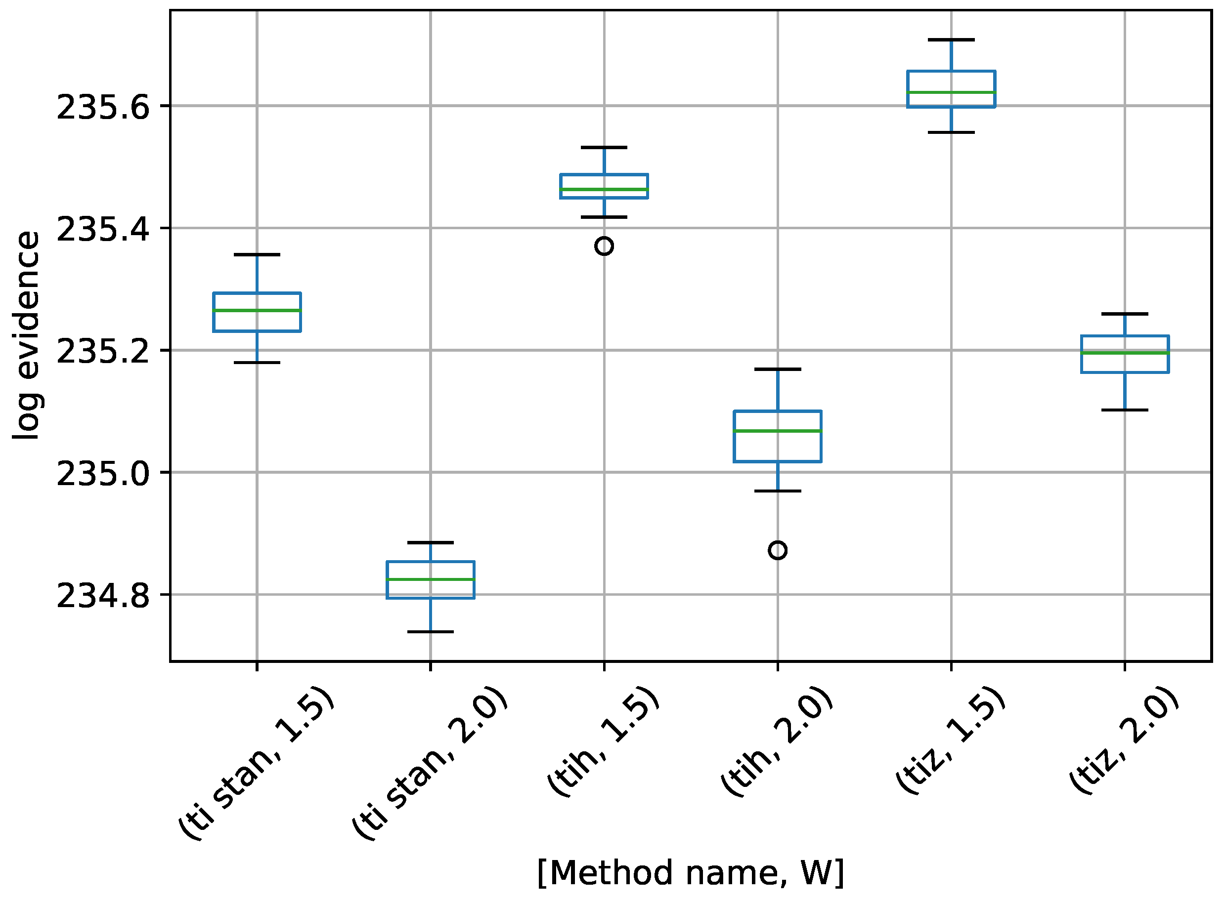
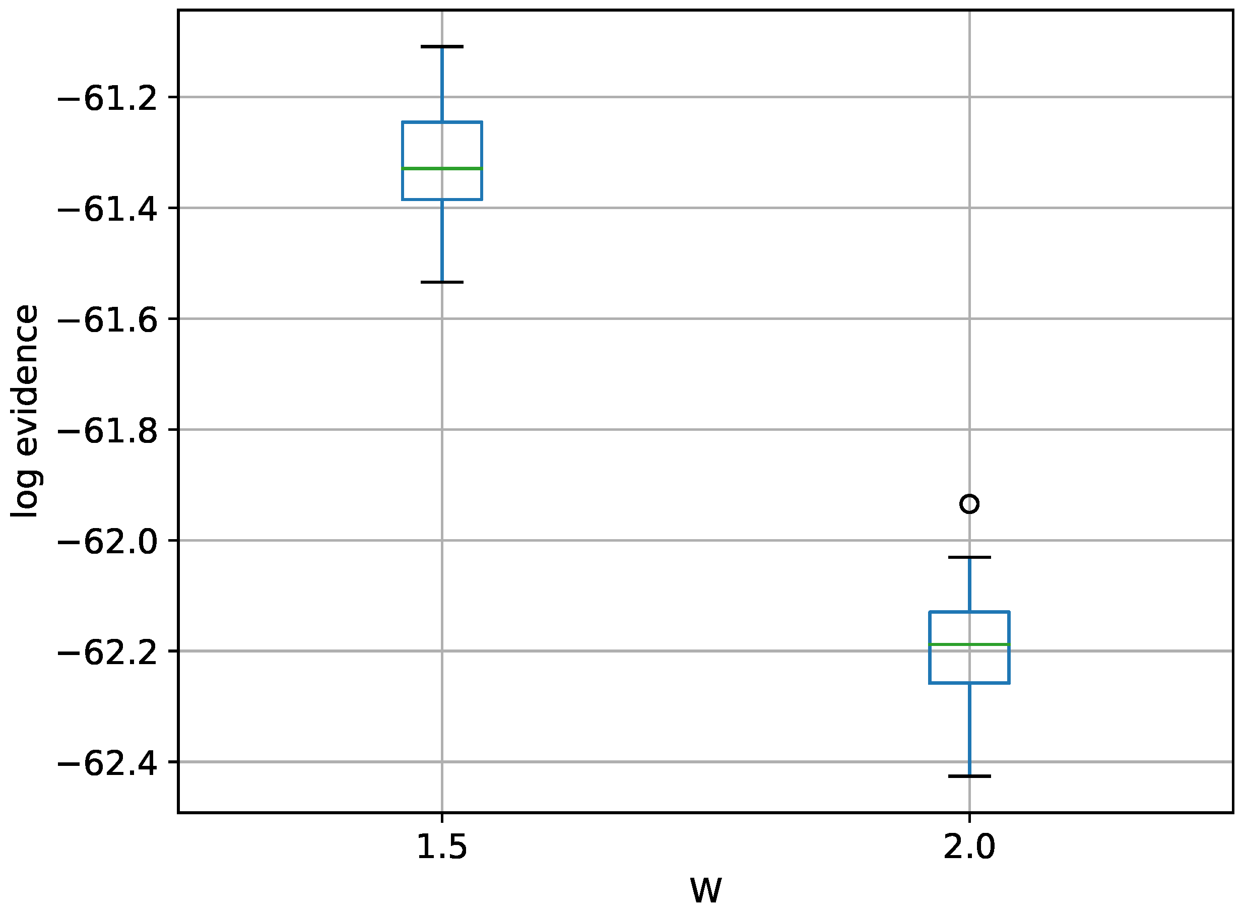
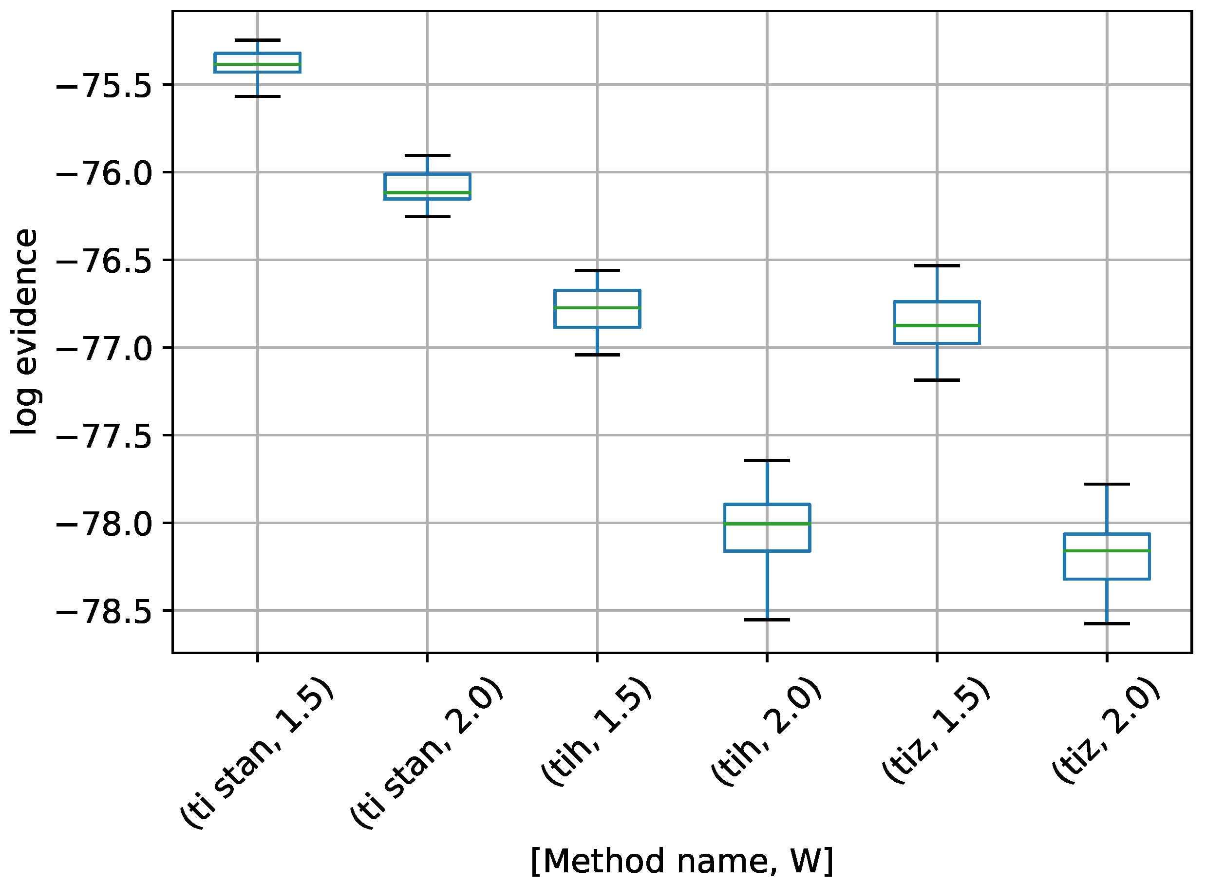
Figure 14.
Box-plot of log-evidence for the one stationary frequency model for TI-Stan, TI-BSS-H, and TI-BSS-Z, for two values of W. TI-Stan with W=xx is denoted by ti stan, xx; TI-BSS-H with W=xx is denoted by tih, xx; and TI-BSS-Z with W=xx is denoted by tiz, xx.
Figure 14.
Box-plot of log-evidence for the one stationary frequency model for TI-Stan, TI-BSS-H, and TI-BSS-Z, for two values of W. TI-Stan with W=xx is denoted by ti stan, xx; TI-BSS-H with W=xx is denoted by tih, xx; and TI-BSS-Z with W=xx is denoted by tiz, xx.
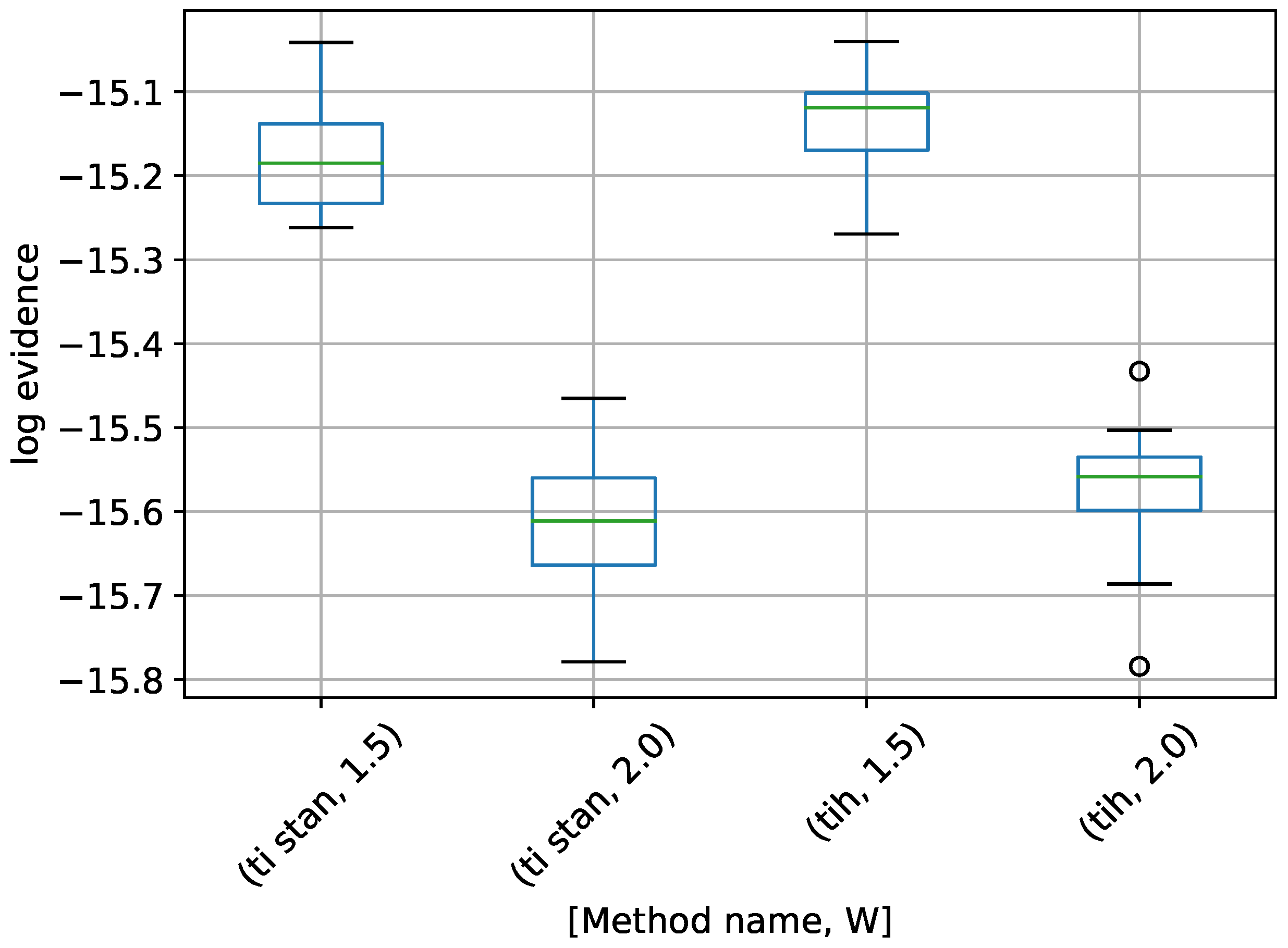
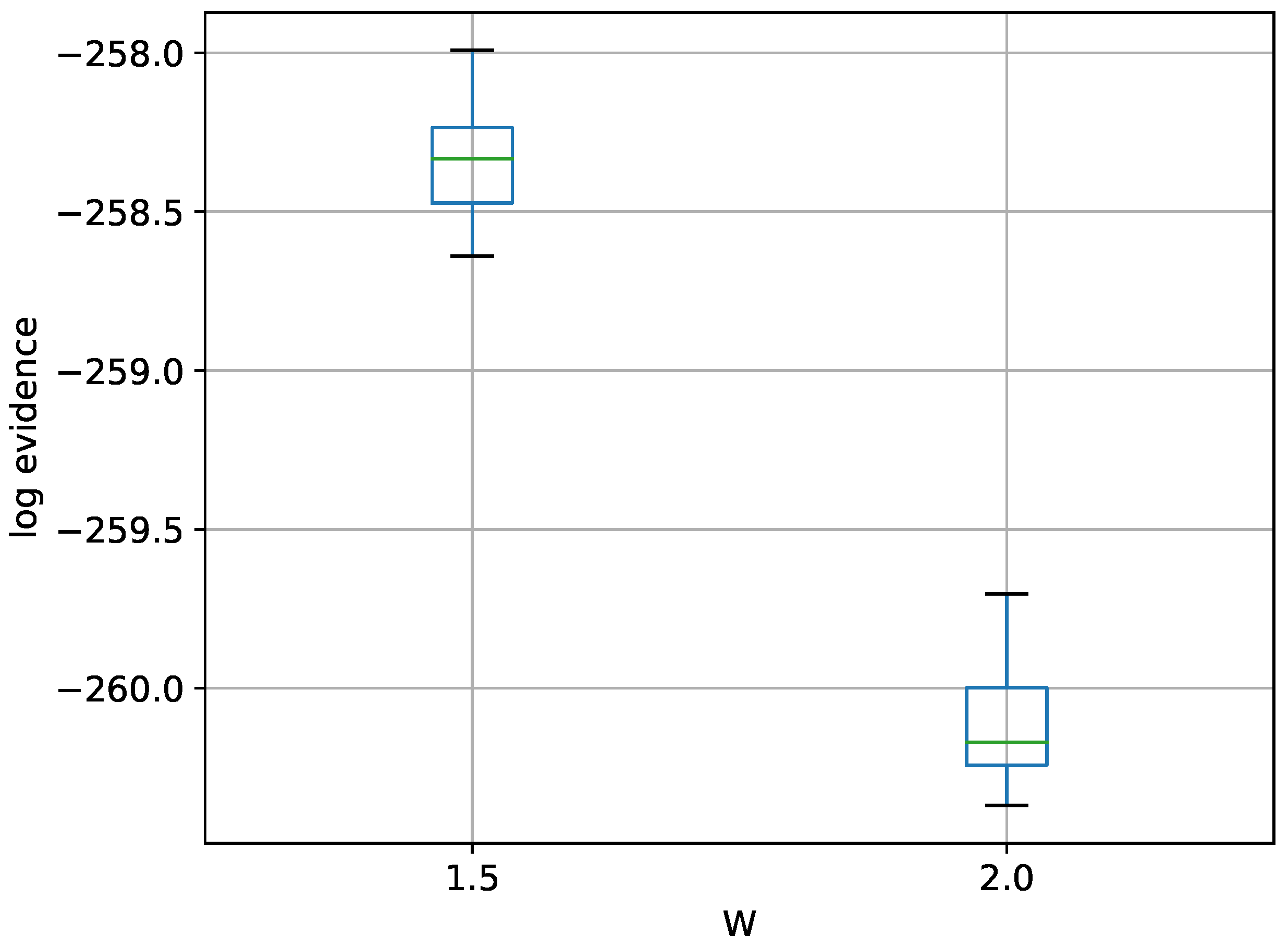
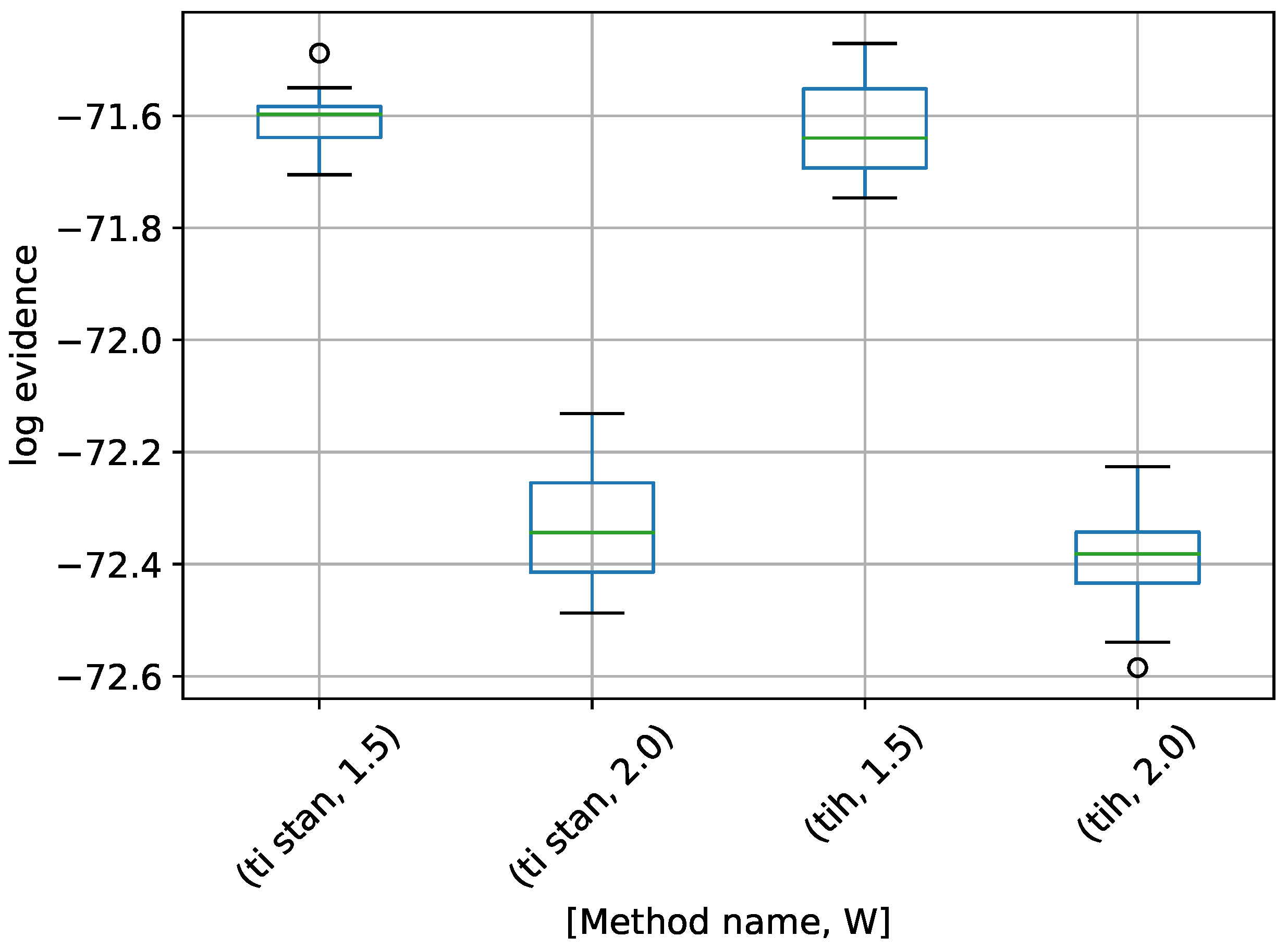
Figure 15.
Box-plot of log-evidence for the two stationary frequency model for TI-Stan and TI-BSS-H, for two values of W. TI-Stan with W=xx is denoted by ti stan, xx and TI-BSS-H with W=xx is denoted by tih, xx.
Figure 15.
Box-plot of log-evidence for the two stationary frequency model for TI-Stan and TI-BSS-H, for two values of W. TI-Stan with W=xx is denoted by ti stan, xx and TI-BSS-H with W=xx is denoted by tih, xx.
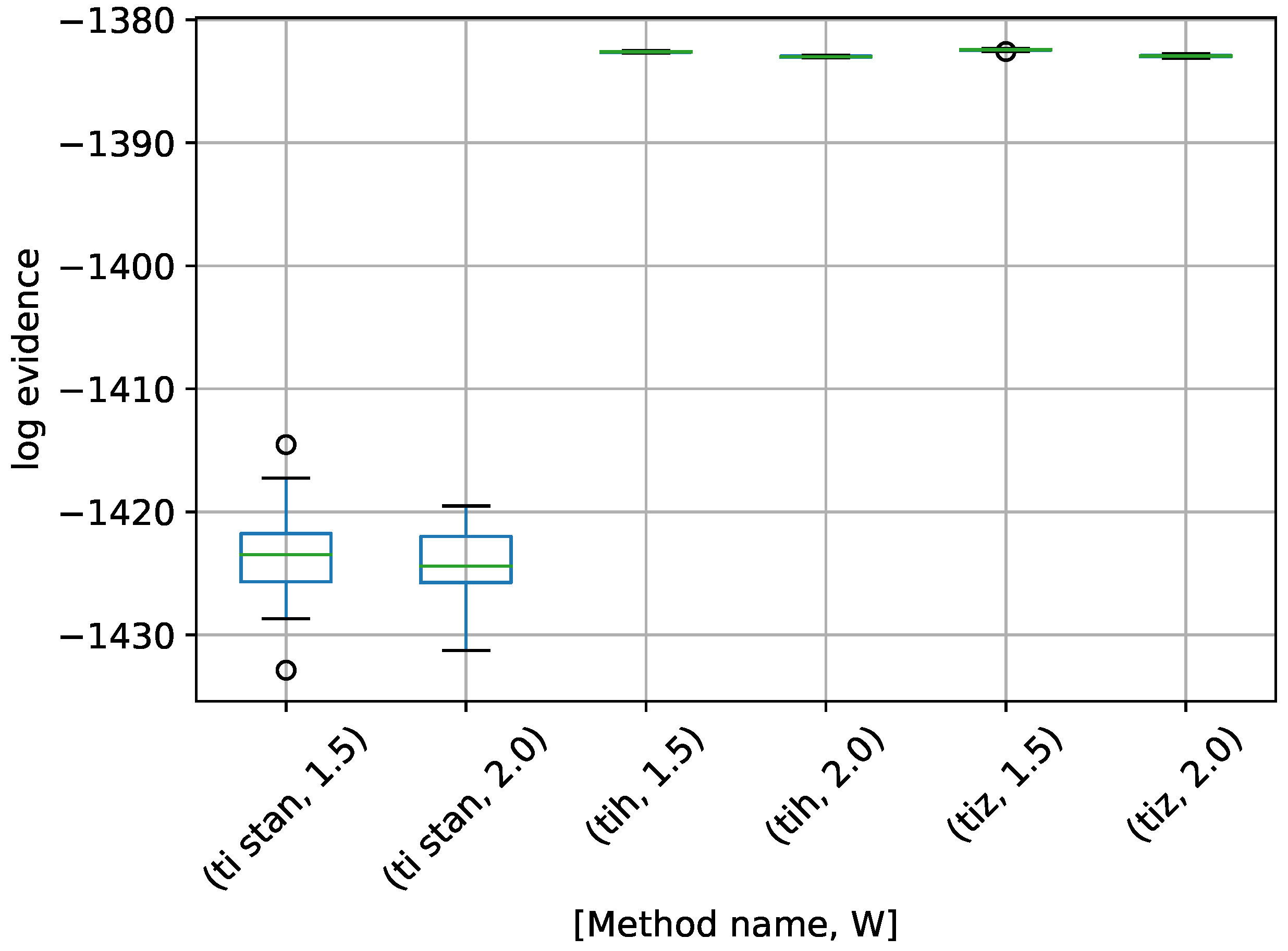
Figure 16.
Box-plot of log-evidence for the three stationary frequency model for TI-Stan, TI-BSS-H, and TI-BSS-Z, for two values of W. TI-Stan with W=xx is denoted by ti stan, xx; TI-BSS-H with W=xx is denoted by tih, xx; and TI-BSS-Z with W=xx is denoted by tiz, xx.
Figure 16.
Box-plot of log-evidence for the three stationary frequency model for TI-Stan, TI-BSS-H, and TI-BSS-Z, for two values of W. TI-Stan with W=xx is denoted by ti stan, xx; TI-BSS-H with W=xx is denoted by tih, xx; and TI-BSS-Z with W=xx is denoted by tiz, xx.
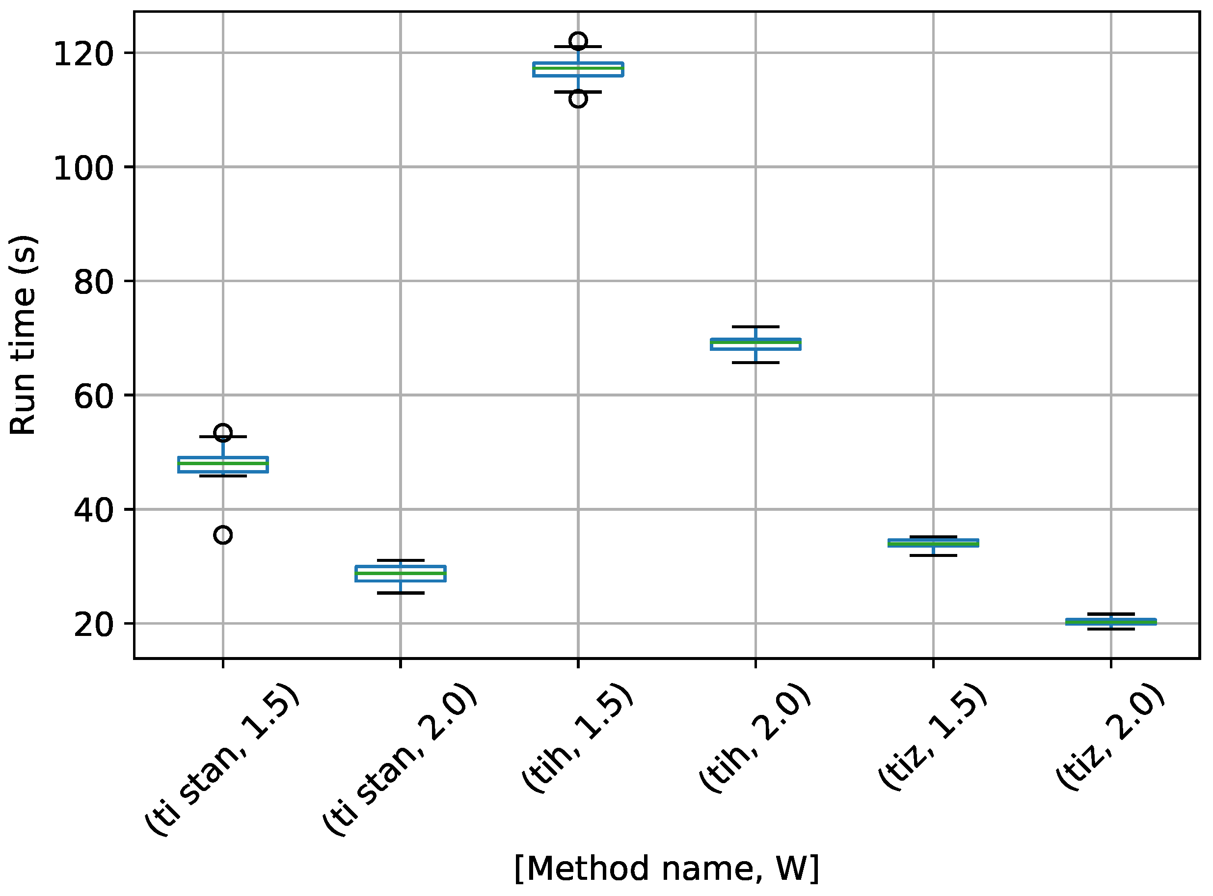
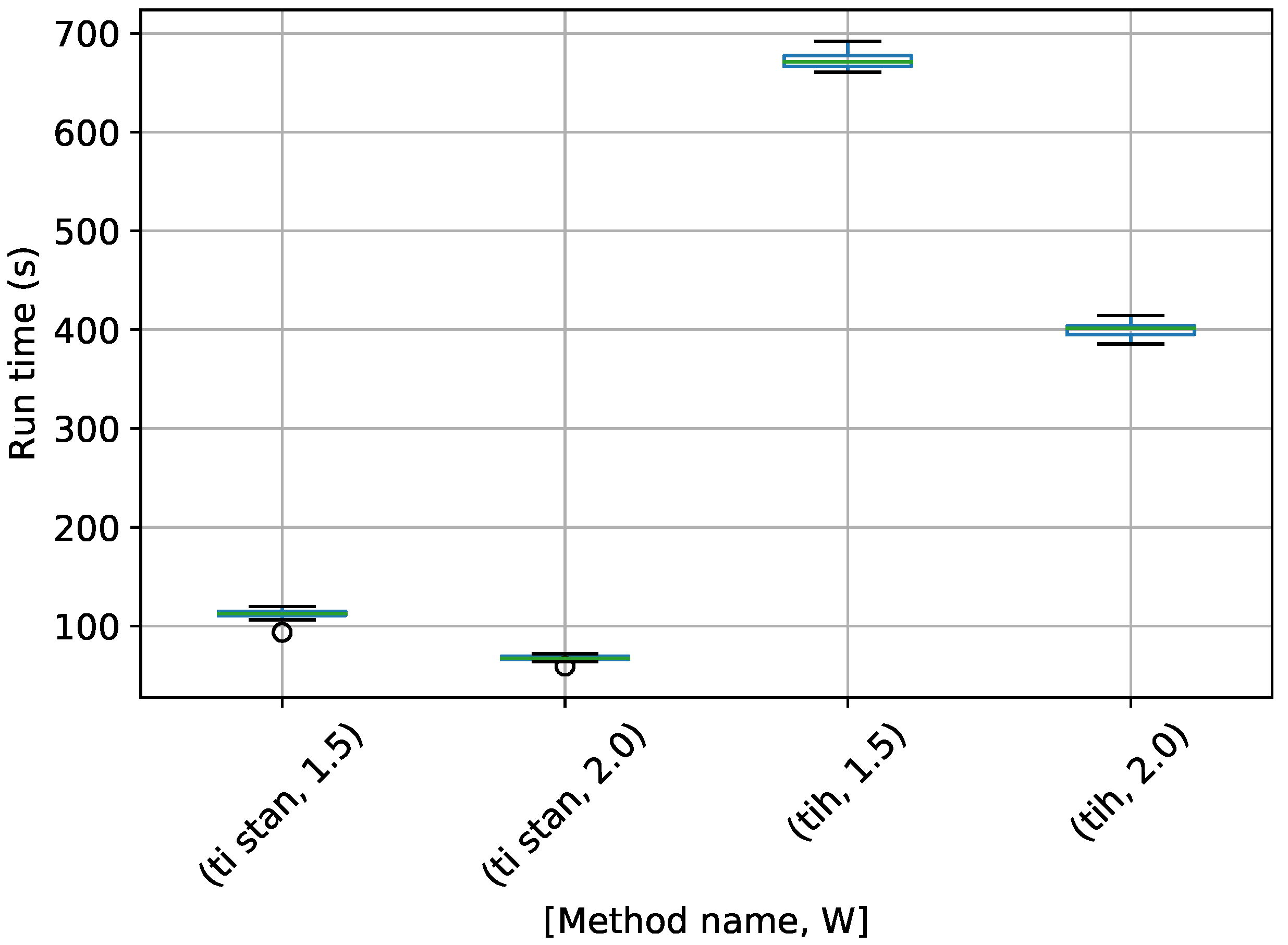
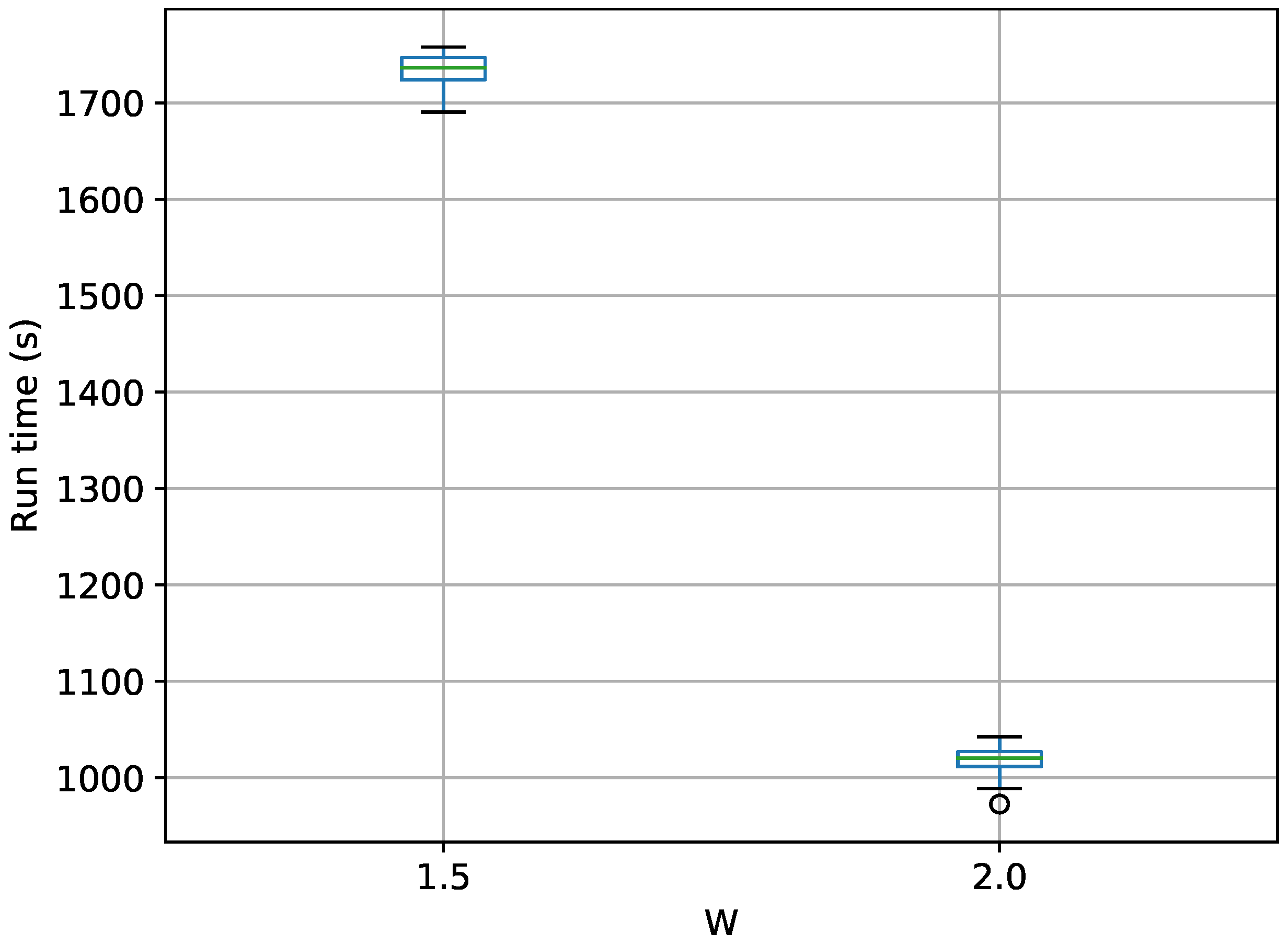
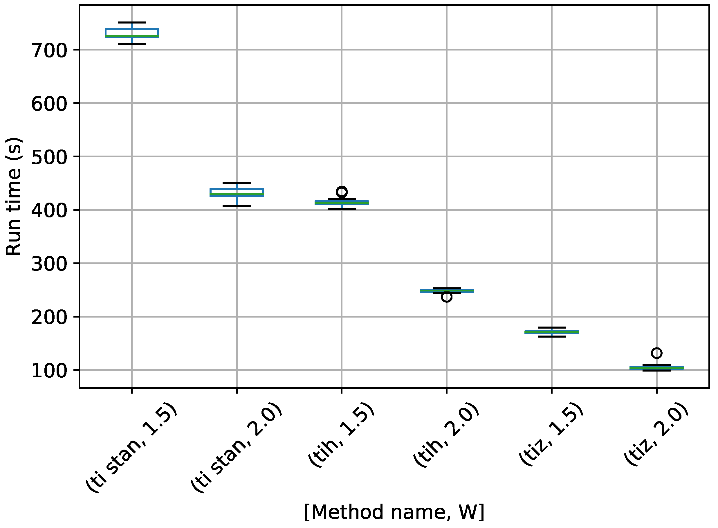
Figure 17.
Box-plot of run time for the stationary frequency model for TI-Stan, TI-BSS-H, and TI-BSS-Z, for two values of W. TI-Stan with W=xx is denoted by ti stan, xx; TI-BSS-H with W=xx is denoted by tih, xx; and TI-BSS-Z with W=xx is denoted by tiz, xx.
Figure 17.
Box-plot of run time for the stationary frequency model for TI-Stan, TI-BSS-H, and TI-BSS-Z, for two values of W. TI-Stan with W=xx is denoted by ti stan, xx; TI-BSS-H with W=xx is denoted by tih, xx; and TI-BSS-Z with W=xx is denoted by tiz, xx.
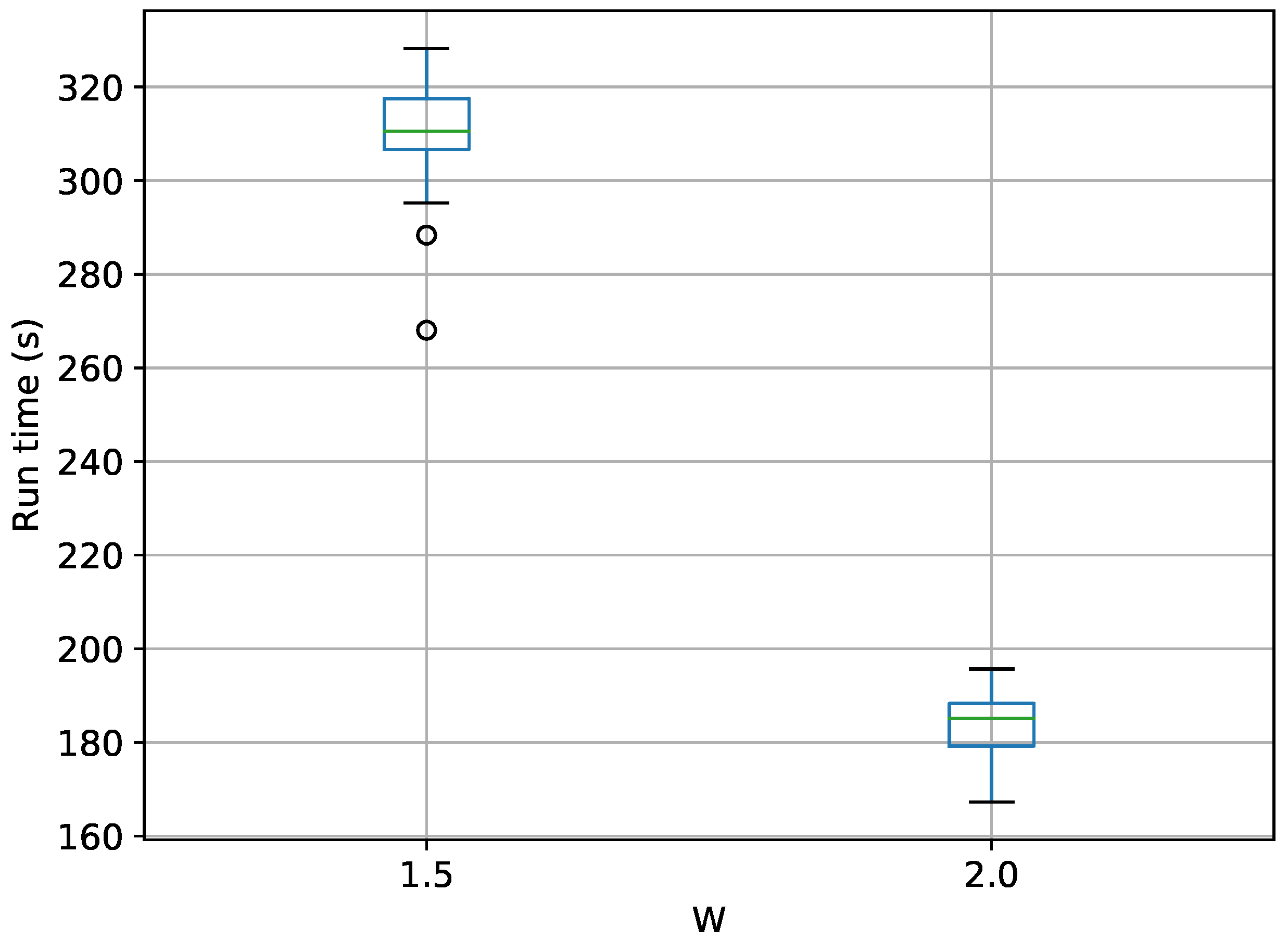
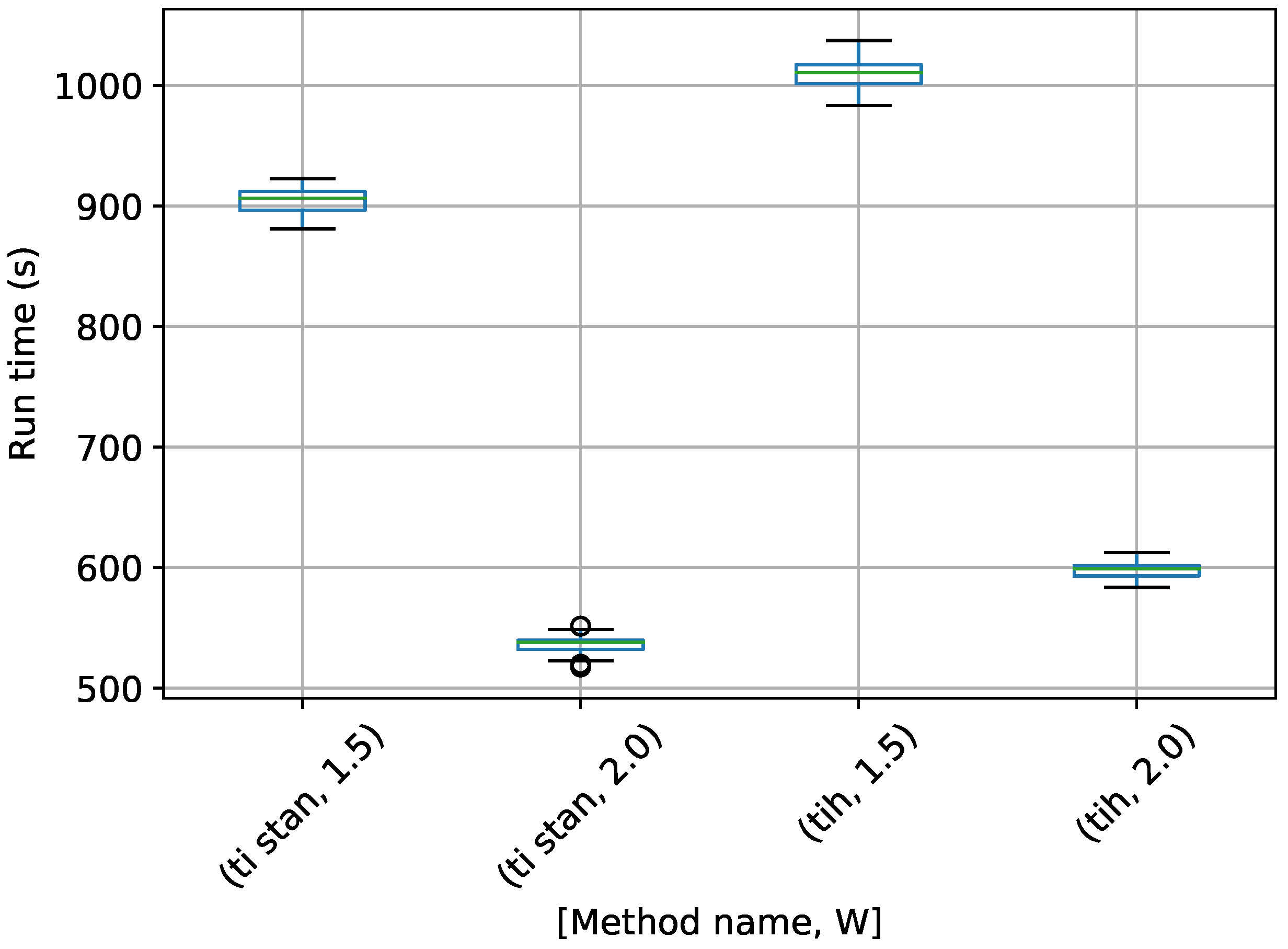
Figure 18.
Box-plot of run time for the stationary frequency model for TI-Stan and TI-BSS-H, for two values of W. TI-Stan with W=xx is denoted by ti stan, xx; and TI-BSS-H with W=xx is denoted by tih, xx.
Figure 18.
Box-plot of run time for the stationary frequency model for TI-Stan and TI-BSS-H, for two values of W. TI-Stan with W=xx is denoted by ti stan, xx; and TI-BSS-H with W=xx is denoted by tih, xx.
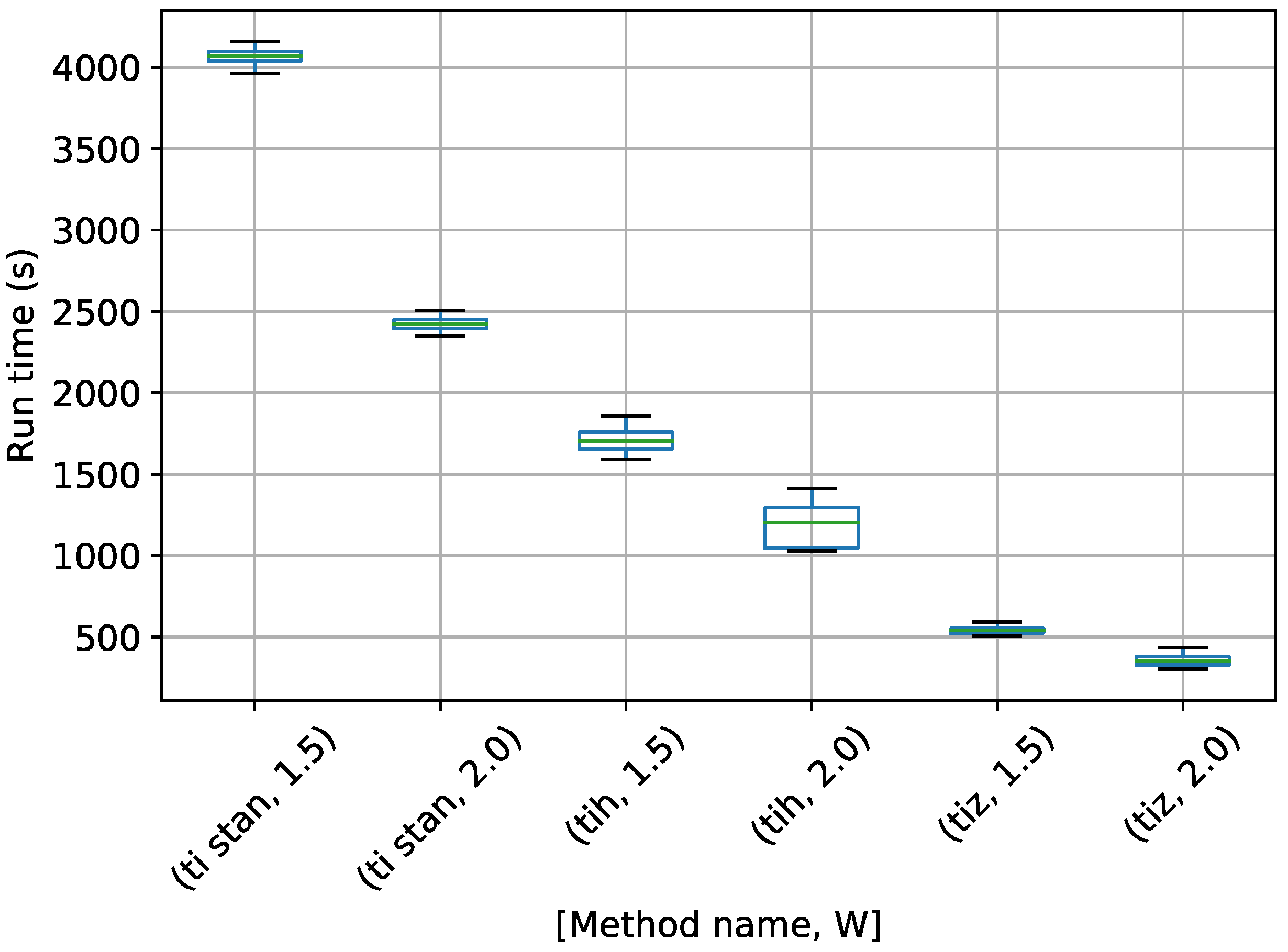
Figure 19.
Box-plot of run time for the stationary frequency model for TI-Stan, TI-BSS-H, and TI-BSS-Z, for two values of W. TI-Stan with W=xx is denoted by ti stan, xx; TI-BSS-H with W=xx is denoted by tih, xx; and TI-BSS-Z with W=xx is denoted by tiz, xx.
Figure 19.
Box-plot of run time for the stationary frequency model for TI-Stan, TI-BSS-H, and TI-BSS-Z, for two values of W. TI-Stan with W=xx is denoted by ti stan, xx; TI-BSS-H with W=xx is denoted by tih, xx; and TI-BSS-Z with W=xx is denoted by tiz, xx.
Table 1.
Prior bounds for multiple stationary frequency model parameters.
Table 1.
Prior bounds for multiple stationary frequency model parameters.
| | Lower Bound | Upper Bound |
|---|
| | 2 |
| | 2 |
| 0 Hz | Hz |
Table 2.
Parameters used to generate simulated signal.
Table 2.
Parameters used to generate simulated signal.
| j | | | (Hz) |
|---|
| 1 | | | |
| 2 | | | |
Table 3.
Parameters for TI-BSS examples.
Table 3.
Parameters for TI-BSS examples.
| Parameter | Value | Definition |
|---|
| S | 200 | Number of binary slice sampling steps |
| M | 2 | Number of combined binary slice sampling and leapfrog steps |
| C | 256 | Number of chains |
| B | 32 | Number of bits per parameter in SFC |
Table 4.
Parameters for TI-Stan examples.
Table 4.
Parameters for TI-Stan examples.
| Parameter | Value | Definition |
|---|
| S | 200 | Number of steps allowed in Stan |
| C | 256 | Number of chains |
Table 5.
Ideal Gas Partition Function results for TI-Stan for two values of W. Twenty TI-Stan runs were completed for each value of W and N.
Table 5.
Ideal Gas Partition Function results for TI-Stan for two values of W. Twenty TI-Stan runs were completed for each value of W and N.
| W | N | Mean Relative Error | StDev Relative Error | Mean | StDev | Analytic (30) |
|---|
| 1.05 | 12 | 0.52% | 0.37% | −12.43 | 0.0565 | −12.49 |
| " | 102 | 0.51% | 0.20% | −118.20 | 0.235 | −118.81 |
| " | 1002 | 0.62% | 0.26% | −1184.16 | 3.04 | −1191.51 |
| 1.5 | 12 | 2.94% | 1.72% | −12.12 | 0.215 | −12.49 |
| " | 102 | 3.39% | 1.44% | −114.78 | 1.71 | −118.81 |
| " | 1002 | 4.50% | 1.40% | −1137.83 | 16.73 | −1191.51 |
Table 6.
Ideal Gas Partition Function run times for TI-Stan for two values of W. Twenty TI-Stan runs were completed for each value of W and N.
Table 6.
Ideal Gas Partition Function run times for TI-Stan for two values of W. Twenty TI-Stan runs were completed for each value of W and N.
| W | N | Mean Run Time (s) | StDev Run Time (s) |
|---|
| 1.05 | 12 | 69.80 | 3.01 |
| " | 102 | 230.56 | 5.74 |
| " | 1002 | 2076.28 | 44.82 |
| 1.5 | 12 | 8.42 | 0.43 |
| " | 102 | 27.87 | 1.44 |
| " | 1002 | 247.53 | 6.80 |


